MQL5での行列およびベクトル演算

特殊なデータ型である行列とベクトルがMQL5言語に追加され、大規模なクラスの数学的問題を解決します。これらの新しい型は、数学表記に近い簡潔でわかりやすいコードを作成するための組み込みメソッドを提供します。この記事では、行列およびベクトルメソッドのヘルプセクションから組み込みメソッドについて簡単に説明します。
内容
- 行列とベクトルの型
- 作成と初期化
- 行列と配列のコピー
- 時系列を行列またはベクトルにコピーする
- 行列演算とベクトル演算
- 操作
- 製品
- 変換
- 統計
- 機能
- 方程式を解く
- 機械学習の手法
- OpenCLの改善
- 機械学習におけるMQL5の未来
すべてのプログラミング言語は、int、doubleなどの数値変数のセットを格納する配列データ型を備えています。配列要素は、ループを使用した配列操作を可能にするインデックスによってアクセスされます。最も一般的に使用されるのは、1次元配列と2次元配列です。
int    a[50];       // One-dimensional array of 50 integers
double m[7][50];    // Two-dimensional array of 7 subarrays, each consisting of 50 integers
MyTime t[100];      // Array containing elements of MyTime type
配列の機能は通常、データの格納と処理に関連する比較的単純なタスクには十分です。しかし、複雑な数学的問題になると、入れ子ループが多数あるため、プログラミングするにもコードを読むにも、配列を扱うするのが難しくなります。最も単純な線形代数操作でさえ、過度のコーディングと数学の十分な理解を必要とします。
機械学習、ニューラルネットワーク、3Dグラフィックスなどの最新のデータテクノロジでは、ベクトルと行列の概念に関連する線形代数の解決策が広く使用されています。このようなオブジェクトの操作を容易にするために、MQL5は特別なデータ型である:行列とベクトルを提供します。これらの新しい型により、多くの日常的なプログラミング操作が不要になり、コードの品質が向上します。
行列型とベクトル型
簡潔に言えば、ベクトルは1次元のdouble型配列であり、行列は2次元のdouble型配列です。ベクトルは垂直および水平にすることができますが、MQL5では分離されていません。
行列は、水平ベクトルの配列として表すことができます。最初のインデックスは行番号で、2番目のインデックスは列番号です。
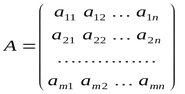
行と列の番号付けは、配列と同様に0から始まります。
double型のデータを含むmatrix型とvector型に加えて、関連するデータ型の演算にはさらに4つの型があります。
この記事の執筆時点では、matrixc型およびvectorc型の作業はまだ完了していないため、組み込みメソッドでこれらの型を使用することはできません。
テンプレート関数は、対応する型の代わりに、matrix<double>、matrix<float>、vector<double>、vector<float>などの表記をサポートします。
  vectorf       v_f1= {0, 1, 2, 3,};
  vector<float> v_f2=v_f1;
  Print("v_f2 = ", v_f2);

  /*
  v_f2 = [0,1,2,3]
  */
作成と初期化
行列メソッドとベクトルメソッドは、その目的に応じて9つのカテゴリに分類されます。行列とベクトルを宣言して初期化するには、いくつかの方法があります。
最も簡単な作成メソッドは、サイズを指定せずに宣言する、つまりデータのメモリ割り当てを行わないメソッドです。ここでは、データ型と変数名を書くだけです。
  matrix         matrix_a;   // double type matrix
  matrix<double> matrix_a1;  // another way to declare a double matrix, suitable for use in templates
  matrix<float>  matrix_a3;  // float type matrix
  vector         vector_a;   // double type vector
  vector<double> vector_a1;  // another notation to create a double vector
  vector<float>  vector_a3;  // float type vector
次に、作成されたオブジェクトのサイズを変更し、目的の値で埋めることができます。また、組み込みの行列メソッドで使用して、計算結果を取得することもできます。
行列またはベクトルは、指定されたサイズで宣言でき、データにメモリを割り当てますが何も初期化しません。ここでは、変数名の後に括弧でサイズを指定します。
  matrix         matrix_a(128,128);           // the parameters can be either constants
  matrix<double> matrix_a1(InpRows,InpCols);  // or variables
  matrix<float>  matrix_a3(InpRows,1);        // analogue of a vertical vector
  vector         vector_a(256);
  vector<double> vector_a1(InpSize);
  vector<float>  vector_a3(InpSize+16);       // expression can be used as a parameter
オブジェクトを作成する3番目の方法は初期化を使用して宣言することです。この場合、行列とベクトルのサイズは、中括弧で示された初期化シーケンスによって決定されます。
  matrix         matrix_a={{0.1,0.2,0.3},{0.4,0.5,0.6}};
  matrix<double> matrix_a1=matrix_a;                      // the matrices must be of the same type
  matrix<float>  matrix_a3={{1,2},{3,4}};
  vector         vector_a={-5,-4,-3,-2,-1,0,1,2,3,4,5};
  vector<double> vector_a1={1,5,2.4,3.3};
  vector<float>  vector_a3=vector_a2;                     // the vectors must be of the same type
特定の方法で初期化された、指定されたサイズの行列とベクトルを作成する静的メソッドもあります。
  matrix         matrix_a =matrix::Eye(4,5,1);
  matrix<double> matrix_a1=matrix::Full(3,4,M_PI);
  matrixf        matrix_a2=matrixf::Identity(5,5);
  matrixf<float> matrix_a3=matrixf::Ones(5,5);
  matrix         matrix_a4=matrix::Tri(4,5,-1);
  vector         vector_a =vector::Ones(256);
  vectorf        vector_a1=vector<float>::Zeros(16);
  vector<float>  vector_a2=vectorf::Full(128,float_value);
さらに、指定された値で行列またはベクトルを初期化するための非静的メソッドInitおよびFillがあります。
  matrix m(2, 2);
  m.Fill(10);
  Print("matrix m \n", m);
  /*
  matrix m
  [[10,10]
  [10,10]]
  */
  m.Init(4, 6);
  Print("matrix m \n", m);
  /*
  matrix m
  [[10,10,10,10,0.0078125,32.00000762939453]
  [0,0,0,0,0,0]
  [0,0,0,0,0,0]
  [0,0,0,0,0,0]]
  */
この例では、Initメソッドを使用して、既に初期化されている行列のサイズを変更しました。これにより、すべての新しい要素がランダムな値で埋められました。
Initメソッドの重要な利点は、パラメータで初期化関数を指定して、この規則に従って行列/ベクトル要素を埋めることができることです。次は例です。
void OnStart()
 {
//---
  matrix init(3, 6, MatrixSetValues);
  Print("init = \n", init);
  /*
  Execution result
  init =
  [[1,2,4,8,16,32]
   [64,128,256,512,1024,2048]
   [4096,8192,16384,32768,65536,131072]]
  */
 }
//+------------------------------------------------------------------+
//| Fills the matrix with powers of a number                         |
//+------------------------------------------------------------------+
void MatrixSetValues(matrix& m, double initial=1)
 {
  double value=initial;
  for(ulong r=0; r<m.Rows(); r++)
   {
    for(ulong c=0; c<m.Cols(); c++)
     {
      m[r][c]=value;
      value*=2;
     }
   }
 }
行列と配列のコピー
行列とベクトルはCopyメソッドを使用してコピーできますが、これらのデータ型をコピーするためのより簡単で使い慣れた方法は代入演算子「=」を使用することです。また、Assignメソッドを使用してコピーすることもできます。
//--- copying matrices
  matrix a= {{2, 2}, {3, 3}, {4, 4}};
  matrix b=a+2;
  matrix c;
  Print("matrix a \n", a);
  Print("matrix b \n", b);
  c.Assign(b);
  Print("matrix c \n", c);
  /*
   matrix a
   [[2,2]
    [3,3]
    [4,4]]
   matrix b
   [[4,4]
    [5,5]
    [6,6]]
   matrix c
   [[4,4]
    [5,5]
    [6,6]]
  */
AssignとCopyとの違いは、行列と配列の両方に使用できることです。次の例は、整数配列int_arrをdouble行列にコピーする方法を示しています。結果の行列は、コピーされた配列のサイズに従って自動的に調整されます。
//--- copying an array to a matrix
  matrix double_matrix=matrix::Full(2,10,3.14);
  Print("double_matrix before Assign() \n", double_matrix);
  int int_arr[5][5]= {{1, 2}, {3, 4}, {5, 6}};
  Print("int_arr: ");
  ArrayPrint(int_arr);
  double_matrix.Assign(int_arr);
  Print("double_matrix after Assign(int_arr) \n", double_matrix);
  /*
   double_matrix before Assign()
   [[3.14,3.14,3.14,3.14,3.14,3.14,3.14,3.14,3.14,3.14]
    [3.14,3.14,3.14,3.14,3.14,3.14,3.14,3.14,3.14,3.14]]

   int_arr:
       [,0][,1][,2][,3][,4]
   [0,]   1   2   0   0   0
   [1,]   3   4   0   0   0
   [2,]   5   6   0   0   0
   [3,]   0   0   0   0   0
   [4,]   0   0   0   0   0

   double_matrix after Assign(int_arr)
   [[1,2,0,0,0]
    [3,4,0,0,0]
    [5,6,0,0,0]
    [0,0,0,0,0]
    [0,0,0,0,0]]
  */
 }
Assignメソッドを使用すると、自動化されたサイズと型のキャストにより、配列から行列へのシームレスな移行が可能になります。
時系列を行列またはベクトルにコピーする
価格チャート分析は、MqlRates構造体配列を使用した操作です。MQL5は、そのような価格データ構造体を操作するための新しい方法を備えています。
CopyRatesメソッドは、MqlRates構造体の履歴系列を行列またはベクトルに直接コピーします。したがって、時系列と指標へのアクセスセクションの関数を使用して、必要な時系列を関連する配列に取得する必要を回避できます。また、それらを行列またはベクトルに転送する必要はありません。CopyRatesメソッドを使用すると、1回の呼び出しでクォートを行列またはベクトルに受け取ることができます。銘柄リストの相関行列を計算する方法の例を考えてみましょう。2つの異なる方法を使用してこれらの値を計算し、結果を比較してみましょう。
input int             InBars=100;
input ENUM_TIMEFRAMES InTF=PERIOD_H1;
//+------------------------------------------------------------------+
//| Script program start function                                    |
//+------------------------------------------------------------------+
void OnStart()
 {
//--- list of symbols for calculation
  string symbols[]= {"EURUSD", "GBPUSD", "USDJPY", "USDCAD", "USDCHF"};
  int size=ArraySize(symbols);
//--- matrix and vector to receive Close prices
  matrix rates(InBars, size);
  vector close;
  for(int i=0; i<size; i++)
   {
    //--- get Close prices to a vector
    if(close.CopyRates(symbols[i], InTF, COPY_RATES_CLOSE, 1, InBars))
     {
      //--- insert the vector to the timeseries matrix
      rates.Col(close, i);
      PrintFormat("%d. %s: %d Close prices were added to matrix", i+1, symbols[i], close.Size());
      //--- output the first 20 vector values for debugging
      int  digits=(int)SymbolInfoInteger(symbols[i], SYMBOL_DIGITS);
      Print(VectorToString(close, 20, digits));
     }
    else
     {
      Print("vector.CopyRates(%d,COPY_RATES_CLOSE) failed. Error ", symbols[i], GetLastError());
      return;
     }
   }
  /*
  1. EURUSD: 100 Close prices were added to the matrix
  0.99561 0.99550 0.99674 0.99855 0.99695 0.99555 0.99732 1.00305 1.00121   1.069 0.99936   1.027 1.00130 1.00129 1.00123 1.00201 1.00222 1.00111   1.079   1.030  ...
  2. GBPUSD: 100 Close prices were added to the matrix
  1.13733 1.13708 1.13777 1.14045 1.13985 1.13783 1.13945 1.14315 1.14172 1.13974 1.13868 1.14116 1.14239 1.14230 1.14160 1.14281 1.14338 1.14242 1.14147 1.14069  ...
  3. USDJPY: 100 Close prices were added to the matrix
  143.451 143.356 143.310 143.202 143.079 143.294 143.146 142.963 143.039 143.032 143.039 142.957 142.904 142.956 142.920 142.837 142.756 142.928 143.130 143.069  ...
  4. USDCAD: 100 Close prices were added to the matrix
  1.32840 1.32877 1.32838 1.32660 1.32780 1.33068 1.33001 1.32798 1.32730 1.32782 1.32951 1.32868 1.32716 1.32663 1.32629 1.32614 1.32586 1.32578 1.32650 1.32789  ...
  5. USDCHF: 100 Close prices were added to the matrix
  0.96395 0.96440 0.96315 0.96161 0.96197 0.96337 0.96358 0.96228 0.96474 0.96529 0.96529 0.96502 0.96463 0.96429 0.96378 0.96377 0.96314 0.96428 0.96483 0.96509  ...
  */
//--- prepare a matrix of correlations between symbols
  matrix corr_from_vector=matrix::Zeros(size, size);
  Print("Compute pairwise correlation coefficients");
  for(int i=0; i<size; i++)
   {
    for(int k=i; k<size; k++)
     {
      vector v1=rates.Col(i);
      vector v2=rates.Col(k);
      double coeff = v1.CorrCoef(v2);
      PrintFormat("corr(%s,%s) = %.3f", symbols[i], symbols[k], coeff);
      corr_from_vector[i][k]=coeff;
     }
   }
  Print("Correlation matrix on vectors: \n", corr_from_vector);
  /*
  Calculate pairwise correlation coefficients
  corr(EURUSD,EURUSD) = 1.000
  corr(EURUSD,GBPUSD) = 0.974
  corr(EURUSD,USDJPY) = -0.713
  corr(EURUSD,USDCAD) = -0.950
  corr(EURUSD,USDCHF) = -0.397
  corr(GBPUSD,GBPUSD) = 1.000
  corr(GBPUSD,USDJPY) = -0.744
  corr(GBPUSD,USDCAD) = -0.953
  corr(GBPUSD,USDCHF) = -0.362
  corr(USDJPY,USDJPY) = 1.000
  corr(USDJPY,USDCAD) = 0.736
  corr(USDJPY,USDCHF) = 0.083
  corr(USDCAD,USDCAD) = 1.000
  corr(USDCAD,USDCHF) = 0.425
  corr(USDCHF,USDCHF) = 1.000

  Correlation matrix on vectors:
  [[1,0.9736363791537366,-0.7126365191640618,-0.9503129578410202,-0.3968181226230434]
   [0,1,-0.7440448047501974,-0.9525190338388175,-0.3617774666815978]
   [0,0,1,0.7360546499847362,0.08314381248168941]
   [0,0,0,0.9999999999999999,0.4247042496841555]
   [0,0,0,0,1]]
  */
//--- now let's see how a correlation matrix can be calculated in one line
  matrix corr_from_matrix=rates.CorrCoef(false);   // false means that the vectors are in the matrix columns
  Print("Correlation matrix rates.CorrCoef(false): \n", corr_from_matrix.TriU());
//--- compare the resulting matrices to find discrepancies
  Print("How many discrepancy errors between result matrices?");
  ulong errors=corr_from_vector.Compare(corr_from_matrix.TriU(), (float)1e-12);
  Print("corr_from_vector.Compare(corr_from_matrix,1e-12)=", errors);
  /*
  Correlation matrix rates.CorrCoef(false):
  [[1,0.9736363791537366,-0.7126365191640618,-0.9503129578410202,-0.3968181226230434]
   [0,1,-0.7440448047501974,-0.9525190338388175,-0.3617774666815978]
   [0,0,1,0.7360546499847362,0.08314381248168941]
   [0,0,0,1,0.4247042496841555]
   [0,0,0,0,1]]

  How many discrepancy errors between result matrices?
  corr_from_vector.Compare(corr_from_matrix,1e-12)=0
  */
//--- create a nice output of the correlation matrix
  Print("Output the correlation matrix with headers");
  string header="        ";  // header
  for(int i=0; i<size; i++)
    header+="  "+symbols[i];
  Print(header);
//--- now rows
  for(int i=0; i<size; i++)
   {
    string line=symbols[i]+"  ";
    line+=VectorToString(corr_from_vector.Row(i), size, 3, 8);
    Print(line);
   }
  /*
  Output the correlation matrix with headers
            EURUSD  GBPUSD  USDJPY  USDCAD  USDCHF
  EURUSD       1.0   0.974  -0.713  -0.950  -0.397
  GBPUSD       0.0     1.0  -0.744  -0.953  -0.362
  USDJPY       0.0     0.0     1.0   0.736   0.083
  USDCAD       0.0     0.0     0.0     1.0   0.425
  USDCHF       0.0     0.0     0.0     0.0     1.0
  */
 }
//+------------------------------------------------------------------+
//| Returns a string with vector values                              |
//+------------------------------------------------------------------+
string VectorToString(const vector &v, int length=20, int digits=5, int width=8)
 {
  ulong size=(ulong)MathMin(20, v.Size());
//--- compose a string
  string line="";
  for(ulong i=0; i<size; i++)
   {
    string value=DoubleToString(v[i], digits);
    StringReplace(value, ".000", ".0");
    line+=Indent(width-StringLen(value))+value;
   }
  //--- add a tail if the vector length exceeds the specified size
  if(v.Size()>size)
    line+="  ...";
//---
  return(line);
 }
//+------------------------------------------------------------------+
//|  Returns a string with the specified number of spaces            |
//+------------------------------------------------------------------+
string Indent(int number)
 {
  string indent="";
  for(int i=0; i<number; i++)
    indent+=" ";
  return(indent);
 }
この例は、次の方法を示しています。
- CopyRatesを使用して終値を取得する
- Colメソッドを使用して行列にベクトルを挿入する
- CorrCoefを使用して2つのベクトル間の相関係数を計算する
- CorrCoefを使用して値ベクトルを含む行列の相関行列を計算する
- TriUメソッドを使用して上三角行列を返す
- 2つの行列を比較し、Compareを使用して不一致を見つける
行列演算とベクトル演算
加算、減算、乗算、除算の要素単位の数学演算は、行列およびベクトルに対して実行できます。このような操作では、両方のオブジェクトが同じタイプとサイズである必要があります。行列またはベクトルの各要素は、2番目の行列またはベクトルの対応する要素に作用します。
適切な型(double、float、complex)のスカラーを2番目の項(乗数、減数、除数)として使用することもできます。この場合、行列またはベクトルの各メンバーは、指定されたスカラーで動作します。
  matrix matrix_a={{0.1,0.2,0.3},{0.4,0.5,0.6}};
  matrix matrix_b={{1,2,3},{4,5,6}};
  matrix matrix_c1=matrix_a+matrix_b;
  matrix matrix_c2=matrix_b-matrix_a;
  matrix matrix_c3=matrix_a*matrix_b;   // Hadamard product
  matrix matrix_c4=matrix_b/matrix_a;
  matrix_c1=matrix_a+1;
  matrix_c2=matrix_b-double_value;
  matrix_c3=matrix_a*M_PI;
  matrix_c4=matrix_b/0.1;
//--- operations in place are possible
  matrix_a+=matrix_b;
  matrix_a/=2;
さらに、行列とベクトルは、MathAbs、MathArccos、MathArcsin、MathArctan、MathCeil、MathCos、MathExp、MathFloor、MathLog、MathLog10、MathMod、MathPow、MathRound、MathSin、MathSqrt、MathTan、、MathExpm1、MathLog1p、MathArccosh、MathArcsinh、MathArctanh、MathCosh、MathSinh、MathTanhなど、ほとんどの数学関数に2番目のパラメータとして渡すことができます。このような操作は、行列とベクトルの要素単位の処理を意味します。例:
//---
  matrix a= {{1, 4}, {9, 16}};
  Print("matrix a=\n",a);
  a=MathSqrt(a);
  Print("MatrSqrt(a)=\n",a);
  /*
   matrix a=
   [[1,4]
    [9,16]]
   MatrSqrt(a)=
   [[1,2]
    [3,4]]
  */
MathModおよびMathPowの場合、2番目の要素は、適切なサイズのスカラーまたは行列/ベクトルのいずれかです。
   matrix<T> mat1(128,128);
   matrix<T> mat3(mat1.Rows(),mat1.Cols());
   ulong     n,size=mat1.Rows()*mat1.Cols();
...
   mat2=MathPow(mat1,(T)1.9);
   for(n=0; n<size; n++)
     {
      T res=MathPow(mat1.Flat(n),(T)1.9);
      if(res!=mat2.Flat(n))
         errors++;
     }

   mat2=MathPow(mat1,mat3);
   for(n=0; n<size; n++)
     {
      T res=MathPow(mat1.Flat(n),mat3.Flat(n));
      if(res!=mat2.Flat(n))
         errors++;
     }
...
   vector<T> vec1(16384);
   vector<T> vec3(vec1.Size());
   ulong     n,size=vec1.Size();
...
   vec2=MathPow(vec1,(T)1.9);
   for(n=0; n<size; n++)
     {
      T res=MathPow(vec1[n],(T)1.9);
      if(res!=vec2[n])
         errors++;
     }
   vec2=MathPow(vec1,vec3);
   for(n=0; n<size; n++)
     {
      T res=MathPow(vec1[n],vec3[n]);
      if(res!=vec2[n])
         errors++;
     }
操作
MQL5は、計算を必要としない、行列とベクトルに対する次の基本的な操作をサポートしています。
- 転置
- 行、列、および対角線の抽出
- 行列のサイズ変更と形状変更
- 指定した行と列の入れ替え
- 新しいオブジェクトへのコピー
- 2つのオブジェクトの比較
- 行列を複数の部分行列に分割する
- 並び替え
  matrix a= {{0, 1, 2}, {3, 4, 5}};
  Print("matrix a \n", a);
  Print("a.Transpose() \n", a.Transpose());
  /*
  matrix a
  [[0,1,2]
   [3,4,5]]
  a.Transpose()
  [[0,3]
   [1,4]
   [2,5]]
  */
以下は、Diagメソッドを使用して対角線を設定および抽出する方法を示す例です。
   vector v1={1,2,3};
   matrix m1;
   m1.Diag(v1);
   Print("m1\n",m1);
  /*
  m1
  [[1,0,0]
  [0,2,0]
  [0,0,3]]
  m2
  */

   matrix m2;
   m2.Diag(v1,-1);
   Print("m2\n",m2);
  /*
  m2
  [[0,0,0]
  [1,0,0]
  [0,2,0]
  [0,0,3]]
  */

   matrix m3;
   m3.Diag(v1,1);
   Print("m3\n",m3);
  /*
  m3
  [[0,1,0,0]
  [0,0,2,0]
  [0,0,0,3]]
  */

   matrix m4=matrix::Full(4,5,9);
   m4.Diag(v1,1);
   Print("m4\n",m4);

   Print("diag -1 - ",m4.Diag(-1));
   Print("diag 0 - ",m4.Diag());
   Print("diag 1 - ",m4.Diag(1));
  /*
  m4
  [[9,1,9,9,9]
  [9,9,2,9,9]
  [9,9,9,3,9]
  [9,9,9,9,9]]
  diag -1 - [9,9,9]
  diag 0 - [9,9,9,9]
  diag 1 - [1,2,3,9]
  */
次は、Reshapeメソッドを使用して行列サイズを変更します。
   matrix matrix_a={{1,2,3},{4,5,6},{7,8,9},{10,11,12}};
   Print("matrix_a\n",matrix_a);
  /*
  matrix_a
  [[1,2,3]
   [4,5,6]
   [7,8,9]
   [10,11,12]]

  */

   matrix_a.Reshape(2,6);
   Print("Reshape(2,6)\n",matrix_a);
  /*
  Reshape(2,6)
  [[1,2,3,4,5,6]
   [7,8,9,10,11,12]]
  */

   matrix_a.Reshape(3,5);
   Print("Reshape(3,5)\n",matrix_a);
  /*
  Reshape(3,5)
  [[1,2,3,4,5]
   [6,7,8,9,10]
   [11,12,0,3,0]]
  */

   matrix_a.Reshape(2,4);
   Print("Reshape(2,4)\n",matrix_a);
  /*
  Reshape(2,4)
  [[1,2,3,4]
   [5,6,7,8]]
  */
次は、Vsplitメソッドを使用した行列の垂直分割の例:です。
   matrix matrix_a={{ 1, 2, 3, 4, 5, 6},
                    { 7, 8, 9,10,11,12},
                    {13,14,15,16,17,18}};
   matrix splitted[];
   ulong  parts[]={2,3};

   matrix_a.Vsplit(2,splitted);
   for(uint i=0; i<splitted.Size(); i++)
      Print("splitted ",i,"\n",splitted[i]);
  /*
     splitted 0
     [[1,2,3]
      [7,8,9]
      [13,14,15]]
     splitted 1
     [[4,5,6]
      [10,11,12]
      [16,17,18]]
  */

   matrix_a.Vsplit(3,splitted);
   for(uint i=0; i<splitted.Size(); i++)
      Print("splitted ",i,"\n",splitted[i]);
  /*
     splitted 0
     [[1,2]
      [7,8]
      [13,14]]
     splitted 1
     [[3,4]
      [9,10]
      [15,16]]
     splitted 2
     [[5,6]
      [11,12]
      [17,18]]
*/

   matrix_a.Vsplit(parts,splitted);
   for(uint i=0; i<splitted.Size(); i++)
      Print("splitted ",i,"\n",splitted[i]);
  /*
     splitted 0
     [[1,2]
      [7,8]
      [13,14]]
     splitted 1
     [[3,4,5]
      [9,10,11]
      [15,16,17]]
     splitted 2
     [[6]
      [12]
      [18]]
  */
ColおよびRowメソッドを使用すると、関連する行列要素を取得したり、要素を未割り当ての行列(指定されたサイズのない行列)に挿入したりできます。以下が一例です。
   vector v1={1,2,3};
   matrix m1;
   m1.Col(v1,1);
   Print("m1\n",m1);
  /*
   m1
   [[0,1]
    [0,2]
    [0,3]]
  */

   matrix m2=matrix::Full(4,5,8);
   m2.Col(v1,2);
   Print("m2\n",m2);
  /*
   m2
   [[8,8,1,8,8]
    [8,8,2,8,8]

    [8,8,3,8,8]
    [8,8,8,8,8]]
  */

   Print("col 1 - ",m2.Col(1));
  /*
   col 1 - [8,8,8,8]
  */

   Print("col 2 - ",m2.Col(2));
  /*
   col 1 - [8,8,8,8]  col 2 - [1,2,3,8]
  */
積
行列乗算は、数値計算法で広く使用されている基本的なアルゴリズムの1つです。ニューラルネットワークの畳み込み層における順方向および逆方向伝搬アルゴリズムの多くの実装は、この操作に基づいています。多くの場合、機械学習に費やされる時間の90~95%がこの操作に費やされます。すべての積のメソッドは、言語リファレンスの行列とベクトルの積のセクションで提供されています。
次の例は、MatMulメソッドを使用した2つの行列の乗算を示しています。
   matrix a={{1, 0, 0},
             {0, 1, 0}};
   matrix b={{4, 1},
             {2, 2},
             {1, 3}};
   matrix c1=a.MatMul(b);
   matrix c2=b.MatMul(a);
   Print("c1 = \n", c1);
   Print("c2 = \n", c2);
/*
   c1 =
   [[4,1]
    [2,2]]
   c2 =
   [[4,1,0]
    [2,2,0]
    [1,3,0]]
*/
次は、クロン法を使用した、2つの行列または行列とベクトルのクロネッカー積の例です。
   matrix a={{1,2,3},{4,5,6}};
   matrix b=matrix::Identity(2,2);
   vector v={1,2};

   Print(a.Kron(b));
   Print(a.Kron(v));

  /*
   [[1,0,2,0,3,0]
    [0,1,0,2,0,3]
    [4,0,5,0,6,0]
    [0,4,0,5,0,6]]

   [[1,2,2,4,3,6]
    [4,8,5,10,6,12]]
  */
次は、MQL5の行列とベクトルの記事からのその他の例です。
//--- initialize matrices
   matrix m35, m52;
   m35.Init(3,5,Arange);
   m52.Init(5,2,Arange);
//---
   Print("1. Product of horizontal vector v[3] and matrix m[3,5]");
   vector v3 = {1,2,3};
   Print("On the left v3 = ",v3);
   Print("On the right m35 = \n",m35);
   Print("v3.MatMul(m35) = horizontal vector v[5] \n",v3.MatMul(m35));
   /*
   1. Product of horizontal vector v[3] and matrix m[3,5]
   On the left v3 = [1,2,3]
   On the right m35 =
   [[0,1,2,3,4]
    [5,6,7,8,9]
    [10,11,12,13,14]]
   v3.MatMul(m35) = horizontal vector v[5]
   [40,46,52,58,64]
   */

//--- show that this is really a horizontal vector
   Print("\n2. Product of matrix m[1,3] and matrix m[3,5]");
   matrix m13;
   m13.Init(1,3,Arange,1);
   Print("On the left m13 = \n",m13);
   Print("On the right m35 = \n",m35);
   Print("m13.MatMul(m35) = matrix m[1,5] \n",m13.MatMul(m35));
   /*
   2. Product of matrix m[1,3] and matrix m[3,5]
   On the left m13 =
   [[1,2,3]]
   On the right m35 =
   [[0,1,2,3,4]
    [5,6,7,8,9]
    [10,11,12,13,14]]
   m13.MatMul(m35) = matrix m[1,5]
   [[40,46,52,58,64]]
   */

   Print("\n3. Product of matrix m[3,5] and vertical vector v[5]");
   vector v5 = {1,2,3,4,5};
   Print("On the left m35 = \n",m35);
   Print("On the right v5 = ",v5);
   Print("m35.MatMul(v5) = vertical vector v[3] \n",m35.MatMul(v5));
   /*
   3. Product of matrix m[3,5] and vertical vector v[5]
   On the left m35 =
   [[0,1,2,3,4]
    [5,6,7,8,9]
    [10,11,12,13,14]]
   On the right v5 = [1,2,3,4,5]
   m35.MatMul(v5) = vertical vector v[3]
   [40,115,190]
   */

//--- show that this is really a vertical vector
   Print("\n4. Product of matrix m[3,5] and matrix m[5,1]");
   matrix m51;
   m51.Init(5,1,Arange,1);
   Print("On the left m35 = \n",m35);
   Print("On the right m51 = \n",m51);
   Print("m35.MatMul(m51) = matrix v[3] \n",m35.MatMul(m51));
   /*
   4. Product of matrix m[3,5] and matrix m[5,1]
   On the left m35 =
   [[0,1,2,3,4]
    [5,6,7,8,9]
    [10,11,12,13,14]]
   On the right m51 =
   [[1]
    [2]
    [3]
    [4]
    [5]]
   m35.MatMul(m51) = matrix v[3]
   [[40]
    [115]
    [190]]
   */

   Print("\n5. Product of matrix m[3,5] and matrix m[5,2]");
   Print("On the left m35 = \n",m35);
   Print("On the right m52 = \n",m52);
   Print("m35.MatMul(m52) = matrix m[3,2] \n",m35.MatMul(m52));
   /*
   5. Product of matrix m[3,5] and matrix m[5,2]
   On the left m35 =
   [[0,1,2,3,4]
    [5,6,7,8,9]
    [10,11,12,13,14]]
   On the right m52 =
   [[0,1]
    [2,3]
    [4,5]
    [6,7]
    [8,9]]
   m35.MatMul(m52) = matrix m[3,2]
   [[60,70]
    [160,195]
    [260,320]]
   */

   Print("\n6. Product of horizontal vector v[5] and matrix m[5,2]");
   Print("On the left v5 = \n",v5);
   Print("On the right m52 = \n",m52);
   Print("v5.MatMul(m52) = horizontal vector v[2] \n",v5.MatMul(m52));
   /*
   6. The product of horizontal vector v[5] and matrix m[5,2]
   On the left v5 =
   [1,2,3,4,5]
   On the right m52 =
   [[0,1]
    [2,3]
    [4,5]
    [6,7]
    [8,9]]
   v5.MatMul(m52) = horizontal vector v[2]
   [80,95]
   */

   Print("\n7. Outer() product of horizontal vector v[5] and vertical vector v[3]");
   Print("On the left v5 = \n",v5);
   Print("On the right v3 = \n",v3);
   Print("v5.Outer(v3) = matrix m[5,3] \n",v5.Outer(v3));
   /*
   7. Outer() product of horizontal vector v[5] and vertical vector v[3]
   On the left v5 =
   [1,2,3,4,5]
   On the right v3 =
   [1,2,3]
   v5.Outer(v3) = matrix m[5,3]
   [[1,2,3]
    [2,4,6]
    [3,6,9]
    [4,8,12]
    [5,10,15]]
   */
変換
行列変換は、データ操作でよく使用されます。しかし、多くの複雑な行列演算は、コンピュータの精度が限られているため、効率的または安定して解くことができません。
行列変換(または分解)は、行列を構成要素に分解する方法です。これにより、より複雑な行列演算の計算が容易になります。行列分解法(行列分解法とも呼ばれます)は、線形方程式の解法、逆行列の計算、行列式の計算などの基本的な操作でも、コンピュータの線形代数のバックボーンです。
機械学習では、元の行列を他の3つの行列の積として表現できる特異値分解(SVD)が広く使用されています。SVDは、最小二乗近似から圧縮や画像認識まで、さまざまな問題を解決するために使用されます。
次は、SVD法による特異値分解の例です。
  matrix a= {{0, 1, 2, 3, 4, 5, 6, 7, 8}};
  a=a-4;
  Print("matrix a \n", a);
  a.Reshape(3, 3);
  matrix b=a;
  Print("matrix b \n", b);
//--- execute SVD decomposition
  matrix U, V;
  vector singular_values;
  b.SVD(U, V, singular_values);
  Print("U \n", U);
  Print("V \n", V);
  Print("singular_values = ", singular_values);

// check block
//--- U * singular diagonal * V = A
  matrix matrix_s;
  matrix_s.Diag(singular_values);
  Print("matrix_s \n", matrix_s);
  matrix matrix_vt=V.Transpose();
  Print("matrix_vt \n", matrix_vt);
  matrix matrix_usvt=(U.MatMul(matrix_s)).MatMul(matrix_vt);
  Print("matrix_usvt \n", matrix_usvt);

  ulong errors=(int)b.Compare(matrix_usvt, 1e-9);
  double res=(errors==0);
  Print("errors=", errors);

//---- another check
  matrix U_Ut=U.MatMul(U.Transpose());
  Print("U_Ut \n", U_Ut);
  Print("Ut_U \n", (U.Transpose()).MatMul(U));

  matrix vt_V=matrix_vt.MatMul(V);
  Print("vt_V \n", vt_V);
  Print("V_vt \n", V.MatMul(matrix_vt));
  /*
  matrix a
  [[-4,-3,-2,-1,0,1,2,3,4]]
  matrix b
  [[-4,-3,-2]
   [-1,0,1]
   [2,3,4]]
  U
  [[-0.7071067811865474,0.5773502691896254,0.408248290463863]
   [-6.827109697437648e-17,0.5773502691896253,-0.8164965809277256]
   [0.7071067811865472,0.5773502691896255,0.4082482904638627]]
  V
  [[0.5773502691896258,-0.7071067811865474,-0.408248290463863]
   [0.5773502691896258,1.779939029415334e-16,0.8164965809277258]
   [0.5773502691896256,0.7071067811865474,-0.408248290463863]]
  singular_values = [7.348469228349533,2.449489742783175,3.277709923350408e-17]

  matrix_s
  [[7.348469228349533,0,0]
   [0,2.449489742783175,0]
   [0,0,3.277709923350408e-17]]
  matrix_vt
  [[0.5773502691896258,0.5773502691896258,0.5773502691896256]
   [-0.7071067811865474,1.779939029415334e-16,0.7071067811865474]
   [-0.408248290463863,0.8164965809277258,-0.408248290463863]]
  matrix_usvt
  [[-3.999999999999997,-2.999999999999999,-2]
   [-0.9999999999999981,-5.977974170712231e-17,0.9999999999999974]
   [2,2.999999999999999,3.999999999999996]]
  errors=0

  U_Ut
  [[0.9999999999999993,-1.665334536937735e-16,-1.665334536937735e-16]
   [-1.665334536937735e-16,0.9999999999999987,-5.551115123125783e-17]
   [-1.665334536937735e-16,-5.551115123125783e-17,0.999999999999999]]
  Ut_U
  [[0.9999999999999993,-5.551115123125783e-17,-1.110223024625157e-16]
   [-5.551115123125783e-17,0.9999999999999987,2.498001805406602e-16]
   [-1.110223024625157e-16,2.498001805406602e-16,0.999999999999999]]
  vt_V
  [[1,-5.551115123125783e-17,0]
   [-5.551115123125783e-17,0.9999999999999996,1.110223024625157e-16]
   [0,1.110223024625157e-16,0.9999999999999996]]
  V_vt
  [[0.9999999999999999,1.110223024625157e-16,1.942890293094024e-16]
   [1.110223024625157e-16,0.9999999999999998,1.665334536937735e-16]
   [1.942890293094024e-16,1.665334536937735e-16,0.9999999999999996]
  */
 }
もう1つの一般的に使用される変換は、コレスキー分解です。これは、行列Aが対称で正定の場合、連立一次方程式Ax=bを解くために使用できます。
MQL5では、コレスキー分解はコレスキー法によって実行されます。
  matrix matrix_a= {{5.7998084, -2.1825367}, {-2.1825367, 9.85910595}};
  matrix matrix_l;
  Print("matrix_a\n", matrix_a);

  matrix_a.Cholesky(matrix_l);
  Print("matrix_l\n", matrix_l);
  Print("check\n", matrix_l.MatMul(matrix_l.Transpose()));
  /*
  matrix_a
  [[5.7998084,-2.1825367]
   [-2.1825367,9.85910595]]
  matrix_l
  [[2.408279136645086,0]
   [-0.9062640068544704,3.006291985133859]]
  check
  [[5.7998084,-2.1825367]
   [-2.1825367,9.85910595]]
  */
以下の表は、使用可能なメソッドのリストを示しています。
統計の取得
- 最大値と最小値、および行列/ベクトルでのインデックス
- 要素の和と積、および累積和と積
- 行列/ベクトル値の中央値、平均値、算術平均、加重算術平均
- 標準偏差と要素分散
- 百分位数と分位数
- 指定されたデータ配列で作成された回帰直線からの偏差エラーとしての回帰メトリック
次は、Stdメソッドによる標準偏差の計算例です。
   matrixf matrix_a={{10,3,2},{1,8,12},{6,5,4},{7,11,9}};
   Print("matrix_a\n",matrix_a);

   vectorf cols_std=matrix_a.Std(0);
   vectorf rows_std=matrix_a.Std(1);
   float matrix_std=matrix_a.Std();

   Print("cols_std ",cols_std);
   Print("rows_std ",rows_std);
   Print("std value  ",matrix_std);
   /*
   matrix_a
   [[10,3,2]
    [1,8,12]
    [6,5,4]
    [7,11,9]]
   cols_std [3.2403703,3.0310888,3.9607449]
   rows_std [3.5590262,4.5460606,0.81649661,1.6329932]
   std value  3.452052593231201
   */
次は、Quantileメソッドによる分位数の計算です。
   matrixf matrix_a={{1,2,3},{4,5,6},{7,8,9},{10,11,12}};
   Print("matrix_a\n",matrix_a);

   vectorf cols_percentile=matrix_a.Percentile(50,0);
   vectorf rows_percentile=matrix_a.Percentile(50,1);
   float matrix_percentile=matrix_a.Percentile(50);

   Print("cols_percentile ",cols_percentile);
   Print("rows_percentile ",rows_percentile);
   Print("percentile value  ",matrix_percentile);
   /*
   matrix_a
   [[1,2,3]
    [4,5,6]
    [7,8,9]
    [10,11,12]]
   cols_percentile [5.5,6.5,7.5]
   rows_percentile [2,5,8,11]
   percentile value  6.5
   */
行列特性
特性セクションのメソッドを使用して、次の値を取得します。
- 行列の行数と列数
- 基準と条件番号
- 行列式、ランク、トレース、および行列のスペクトル
次は、Rankメソッドを使用した行列のランクの計算:
  matrix a=matrix::Eye(4, 4);;
  Print("matrix a \n", a);
  Print("a.Rank()=", a.Rank());

  matrix I=matrix::Eye(4, 4);
  I[3, 3] = 0.;    // matrix deficit
  Print("I \n", I);
  Print("I.Rank()=", I.Rank());

  matrix b=matrix::Ones(1, 4);
  Print("b \n", b);
  Print("b.Rank()=", b.Rank());;// 1 size - rank 1, unless all 0

  matrix  zeros=matrix::Zeros(4, 1);
  Print("zeros \n", zeros);
  Print("zeros.Rank()=", zeros.Rank());
  /*
  matrix a
  [[1,0,0,0]
  [0,1,0,0]
  [0,0,1,0]
  [0,0,0,1]]
  a.Rank()=4

  I
  [[1,0,0,0]
  [0,1,0,0]
  [0,0,1,0]
  [0,0,0,0]]
  I.Rank()=3

  b
  [[1,1,1,1]]
  b.Rank()=1

  zeros
  [[0]
  [0]
  [0]
  [0]]
  zeros.Rank()=0
  */
Normメソッドを使用したノルムの計算です。:
  matrix a= {{0, 1, 2, 3, 4, 5, 6, 7, 8}};
  a=a-4;
  Print("matrix a \n", a);
  a.Reshape(3, 3);
  matrix b=a;
  Print("matrix b \n", b);
  Print("b.Norm(MATRIX_NORM_P2)=", b.Norm(MATRIX_NORM_FROBENIUS));
  Print("b.Norm(MATRIX_NORM_FROBENIUS)=", b.Norm(MATRIX_NORM_FROBENIUS));
  Print("b.Norm(MATRIX_NORM_INF)", b.Norm(MATRIX_NORM_INF));
  Print("b.Norm(MATRIX_NORM_MINUS_INF)", b.Norm(MATRIX_NORM_MINUS_INF));
  Print("b.Norm(MATRIX_NORM_P1)=)", b.Norm(MATRIX_NORM_P1));
  Print("b.Norm(MATRIX_NORM_MINUS_P1)=", b.Norm(MATRIX_NORM_MINUS_P1));
  Print("b.Norm(MATRIX_NORM_P2)=", b.Norm(MATRIX_NORM_P2));
  Print("b.Norm(MATRIX_NORM_MINUS_P2)=", b.Norm(MATRIX_NORM_MINUS_P2));
  /*
  matrix a
  [[-4,-3,-2,-1,0,1,2,3,4]]
  matrix b
  [[-4,-3,-2]
  [-1,0,1]
  [2,3,4]]
  b.Norm(MATRIX_NORM_P2)=7.745966692414834
  b.Norm(MATRIX_NORM_FROBENIUS)=7.745966692414834
  b.Norm(MATRIX_NORM_INF)9.0
  b.Norm(MATRIX_NORM_MINUS_INF)2.0
  b.Norm(MATRIX_NORM_P1)=)7.0
  b.Norm(MATRIX_NORM_MINUS_P1)=6.0
  b.Norm(MATRIX_NORM_P2)=7.348469228349533
  b.Norm(MATRIX_NORM_MINUS_P2)=1.857033188519056e-16
  */
方程式を解く
機械学習方法と最適化問題では、多くの場合、線形方程式系の解を見つける必要があります。解決策セクションには、行列の種類に応じて、このような方程式の解を可能にする4つのメソッドが含まれています。
| 関数 | アクション |
|---|---|
| 線形行列方程式または線形代数方程式系を解く | |
| LstSq()-線形代数方程式の最小二乗解を返す(非二乗または縮退行列の場合) | |
| ジョーダン・ガウス法により正方可逆行列の乗法逆行列を算出する | |
| Moore-Penrose法により行列の疑似逆行列を算出する |
方程式A*x=bを解く例を考えてみましょう。

解ベクトルxを見つける必要があります。行列Aは正方形ではないため、ここではSolveメソッドを使用できません。
非正方行列または縮退行列の近似解法を可能にするLstSqメソッドを使用します。
   matrix a={{3, 2},
             {4,-5},
             {3, 3}};
   vector b={7,40,3};
//--- solve the system A*x = b
   vector x=a.LstSq(b);
//--- check the solution, x must be equal to [5, -4]
   Print("x=", x);
  /*
  x=[5.00000000,-4]
  */

//--- check A*x = b1, the resulting vector must be [7, 40, 3]
   vector b1=a.MatMul(x);
   Print("b11=",b1);
/*
  b1=[7.0000000,40.0000000,3.00000000]
*/
チェックすると、検出されたベクトルxがこの連立方程式の解であることが示されました。
機械学習の手法
機械学習で使用できる行列法とベクトル法は3つあります。
| 関数 | アクション |
|---|---|
| 活性化関数の値を計算し、渡されたベクトル/行列に書き込む | |
| 活性化関数の微分値を計算し、渡されたベクトル/行列に書き込む | |
| 損失関数値を計算し、渡されたベクトル/行列に書き込む |
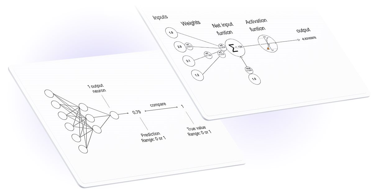
活性化関数はニューラルネットワークで使用され、重み付けされた入力の合計に応じて出力を見つけます。活性化関数の選択は、ニューラルネットワークのパフォーマンスに大きな影響を与えます。
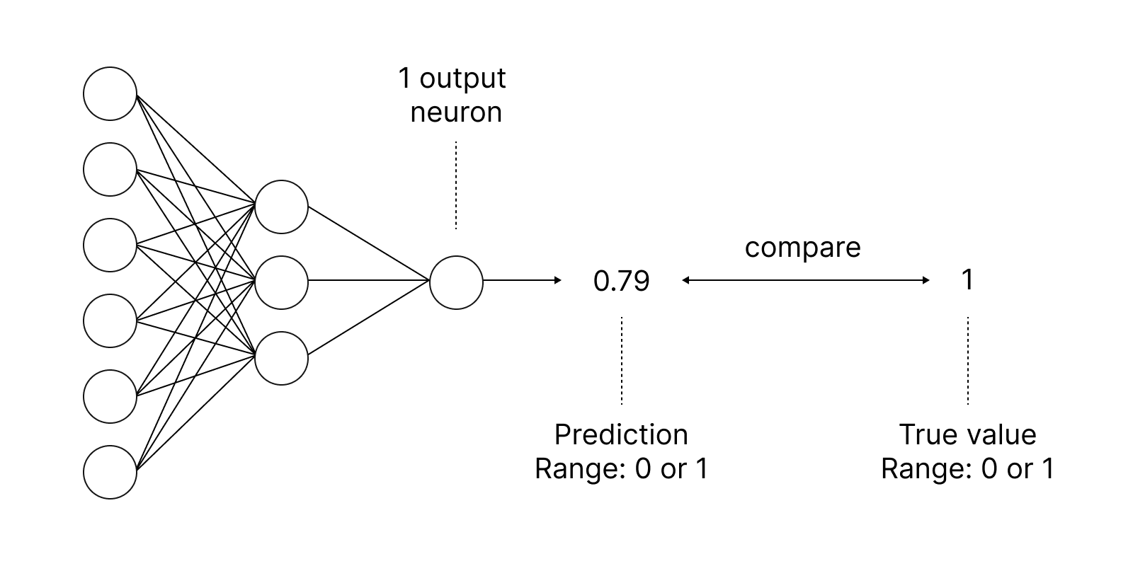
最も一般的な活性化関数の1つはシグモイドです。
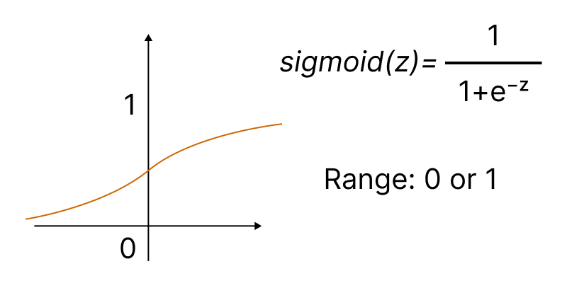
組み込みのActivationメソッドを使用すると、15種類の活性化関数のいずれかを設定できます。それらはすべてENUM_ACTIVATION_FUNCTION列挙で利用できます。
| ID | 詳細 |
|---|---|
| AF_ELU | ELU(指数線形ユニット) |
| AF_EXP | 指数 |
| AF_GELU | ガウス誤差線形単位 |
| AF_HARD_SIGMOID | ハードシグモイド |
| AF_LINEAR | リニア |
| AF_LRELU | LeakyReLU |
| AF_RELU | ReLU(正規化線形ユニット) |
| AF_SELU | ScaledELU(指数線形ユニット) |
| AF_SIGMOID | シグモイド |
| AF_SOFTMAX | Softmax |
| AF_SOFTPLUS | Softplus |
| AF_SOFTSIGN | ソフトサイン |
| AF_SWISH | Swish |
| AF_TANH | 双曲正接関数 |
| AF_TRELU | しきい値処理されたReLU |
ニューラルネットワークは、損失関数を使用して、学習のエラーを最小化するアルゴリズムを見つけることを目的としています。偏差は、ENUM_LOSS_FUNCTION列挙から14種類のいずれかを指定できるLossメソッドを使用して計算されます。
得られた偏差値は、ニューラルネットワークのパラメータを調整するために使用されます。これは、活性化関数の導関数の値を計算し、渡されたベクトル/行列に結果を書き込むDerivativeメソッドを使用しておこなわれます。ニューラルネットワークの訓練プロセスは、「MQL言語を使用したゼロからのディープニューラルネットワークプログラミング」稿のアニメーションを使用して視覚的に表すことができます。
OpenCLの改善
また、CLBufferWrite関数とCLBufferRead関数で行列とベクトルのサポートを実装しました。これらの関数は、対応するオーバーロードを備えています。行列の例を以下に示します。
行列からバッファに値を書き込み、成功するとtrueを返します。
uint  CLBufferWrite(
   int           buffer,                    // OpenCL buffer handle
   uint          buffer_offset,             // offset in the OpenCL buffer in bytes
   matrix<T>     &mat                       // matrix of values to write to buffer
   );
OpenCLバッファを行列に読み取り、成功するとtrueを返します。
uint  CLBufferRead(
   int           buffer,                    // OpenCL buffer handle
   uint          buffer_offset,             // offset in the OpenCL buffer in bytes
   const matrix& mat,                       // matrix to get values from the buffer
   ulong         rows=-1,                   // number of rows in the matrix
   ulong         cols=-1                    // number of columns in the matrix
   );
2つの行列の行列積の例を使用して、新しいオーバーロードの使用を考えてみましょう。次の3つの方法を使用して計算を行います。
- 行列乗算アルゴリズムを説明する単純な方法
- 組み込みのMatMulメソッド
- OpenCLでの並列計算
得られた行列は、指定された精度で2つの行列の要素を比較するCompareメソッドを使用してチェックされます。
#define M       3000      // number of rows in the first matrix
#define K       2000      // number of columns in the first matrix equal to the number of rows in the second one
#define N       3000      // number of columns in the second matrix

//+------------------------------------------------------------------+
const string clSrc=
  "#define N     "+IntegerToString(N)+"                              \r\n"
  "#define K     "+IntegerToString(K)+"                              \r\n"
  "                                                                  \r\n"
  "__kernel void matricesMul( __global float *in1,                   \r\n"
  "                           __global float *in2,                   \r\n"
  "                           __global float *out  )                 \r\n"
  "{                                                                 \r\n"
  "  int m = get_global_id( 0 );                                     \r\n"
  "  int n = get_global_id( 1 );                                     \r\n"
  "  float sum = 0.0;                                                \r\n"
  "  for( int k = 0; k < K; k ++ )                                   \r\n"
  "     sum += in1[ m * K + k ] * in2[ k * N + n ];                  \r\n"
  "  out[ m * N + n ] = sum;                                         \r\n"
  "}                                                                 \r\n";
//+------------------------------------------------------------------+
//| Script program start function                                    |
//+------------------------------------------------------------------+
void OnStart()
 {
//--- initialize the random number generator
  MathSrand((int)TimeCurrent());
//--- fill matrices of the given size with random values
  matrixf mat1(M, K, MatrixRandom) ;    // first matrix
  matrixf mat2(K, N, MatrixRandom);     // second matrix

//--- calculate the product of matrices using the naive way
  uint start=GetTickCount();
  matrixf matrix_naive=matrixf::Zeros(M, N);// here we rite the result of multiplying two matrices
  for(int m=0; m<M; m++)
    for(int k=0; k<K; k++)
      for(int n=0; n<N; n++)
        matrix_naive[m][n]+=mat1[m][k]*mat2[k][n];
  uint time_naive=GetTickCount()-start;

//--- calculate the product of matrices using MatMull
  start=GetTickCount();
  matrixf matrix_matmul=mat1.MatMul(mat2);
  uint time_matmul=GetTickCount()-start;

//--- calculate the product of matrices in OpenCL
  matrixf matrix_opencl=matrixf::Zeros(M, N);
  int cl_ctx;             // context handle
  if((cl_ctx=CLContextCreate(CL_USE_GPU_ONLY))==INVALID_HANDLE)
   {
    Print("OpenCL not found, exit");
    return;
   }
  int cl_prg;             // program handle
  int cl_krn;             // kernel handle
  int cl_mem_in1;         // handle of the first buffer (input)
  int cl_mem_in2;         // handle of the second buffer (input)
  int cl_mem_out;         // handle of the third buffer (output)
//--- create the program and the kernel
  cl_prg = CLProgramCreate(cl_ctx, clSrc);
  cl_krn = CLKernelCreate(cl_prg, "matricesMul");
//--- create all three buffers for the three matrices
  cl_mem_in1=CLBufferCreate(cl_ctx, M*K*sizeof(float), CL_MEM_READ_WRITE);
  cl_mem_in2=CLBufferCreate(cl_ctx, K*N*sizeof(float), CL_MEM_READ_WRITE);
//--- third matrix - output
  cl_mem_out=CLBufferCreate(cl_ctx, M*N*sizeof(float), CL_MEM_READ_WRITE);
//--- set kernel arguments
  CLSetKernelArgMem(cl_krn, 0, cl_mem_in1);
  CLSetKernelArgMem(cl_krn, 1, cl_mem_in2);
  CLSetKernelArgMem(cl_krn, 2, cl_mem_out);
//--- write matrices to device buffers
  CLBufferWrite(cl_mem_in1, 0, mat1);
  CLBufferWrite(cl_mem_in2, 0, mat2);
  CLBufferWrite(cl_mem_out, 0, matrix_opencl);
//--- start the OpenCL code execution time
  start=GetTickCount();
//--- set the task workspace parameters and execute the OpenCL program
  uint  offs[2] = {0, 0};
  uint works[2] = {M, N};
  start=GetTickCount();
  bool ex=CLExecute(cl_krn, 2, offs, works);
//--- read the result into the matrix
  if(CLBufferRead(cl_mem_out, 0, matrix_opencl))
    PrintFormat("Matrix [%d x %d] read ", matrix_opencl.Rows(), matrix_opencl.Cols());
   else
      Print("CLBufferRead(cl_mem_out, 0, matrix_opencl failed. Error ",GetLastError());
  uint time_opencl=GetTickCount()-start;
  Print("Compare computation times of the methods");
  PrintFormat("Naive product time = %d ms",time_naive);
  PrintFormat("MatMul product time = %d ms",time_matmul);
  PrintFormat("OpenCl product time = %d ms",time_opencl);
//--- release all OpenCL contexts
  CLFreeAll(cl_ctx, cl_prg, cl_krn, cl_mem_in1, cl_mem_in2, cl_mem_out);

//--- compare all obtained result matrices with each other
  Print("How many discrepancy errors between result matrices?");
  ulong errors=matrix_naive.Compare(matrix_matmul,(float)1e-12);
  Print("matrix_direct.Compare(matrix_matmul,1e-12)=",errors);
  errors=matrix_matmul.Compare(matrix_opencl,float(1e-12));
  Print("matrix_matmul.Compare(matrix_opencl,1e-12)=",errors);
/*
   Result:

   Matrix [3000 x 3000] read
   Compare computation times of the methods
   Naive product time = 54750 ms
   MatMul product time = 4578 ms
   OpenCl product time = 922 ms
   How many discrepancy errors between result matrices?
   matrix_direct.Compare(matrix_matmul,1e-12)=0
   matrix_matmul.Compare(matrix_opencl,1e-12)=0
*/
 }
//+------------------------------------------------------------------+
//| Fills the matrix with random values                              |
//+------------------------------------------------------------------+
void MatrixRandom(matrixf& m)
 {
  for(ulong r=0; r<m.Rows(); r++)
   {
    for(ulong c=0; c<m.Cols(); c++)
     {
      m[r][c]=(float)((MathRand()-16383.5)/32767.);
     }
   }
 }
//+------------------------------------------------------------------+
//| Release all OpenCL contexts                                      |
//+------------------------------------------------------------------+
void CLFreeAll(int cl_ctx, int cl_prg, int cl_krn,
               int cl_mem_in1, int cl_mem_in2, int cl_mem_out)
 {
//--- release all created OpenCL contexts in reverse order
  CLBufferFree(cl_mem_in1);
  CLBufferFree(cl_mem_in2);
  CLBufferFree(cl_mem_out);
  CLKernelFree(cl_krn);
  CLProgramFree(cl_prg);
  CLContextFree(cl_ctx);
 }
この例のOpenCLコードの詳細な説明は、「OpenCL:ネィティブから、より洞察力のあるプログラミングへ」稿にあります。
その他の改善
ビルド3390では、GPUの使用に影響するOpenCL操作の2つの制限が解除されました。
特定のタスクを二重にサポートするGPUの必須使用を設定するには、CLContextCreate呼び出しでCL_USE_GPU_DOUBLE_ONLYを使用します。
   int cl_ctx;
//--- initialization of OpenCL context
   if((cl_ctx=CLContextCreate(CL_USE_GPU_DOUBLE_ONLY))==INVALID_HANDLE)
     {
      Print("OpenCL not found");
      return;
     }
OpenCL操作の変更は、行列やベクトルに直接関係していませんが、MQL5言語の機械学習機能を開発する取り組みと一致しています。
機械学習におけるMQL5の未来
過去数年間、MQL5言語に高度な技術を導入するために多くのことを行ってきました。
- 数値計算法のALGLIBライブラリのMQL5への移植
- ファジーロジックと統計手法を使用した数学ライブラリの実装
- プロット関数の類似物であるグラフィックライブラリの紹介
- Pythonと統合した、Pythonスクリプトのターミナルでの直接実行
- 3Dグラフィックスを作成するためのDirectX関数の追加
- データベース操作のためのネイティブSQLiteサポートの実装
- 新しいデータ型である行列とベクトルおよび必要なすべてのメソッドの追加
MQL5言語は引き続き開発されますが、最優先方向の1つは機械学習です。私たちはさらなる発展のための大きな計画を持っています。私たちをサポートし、私たちと一緒に学び続けてください。
MetaQuotes Ltdによってロシア語から翻訳されました。
元の記事: https://www.mql5.com/ru/articles/10922
警告: これらの資料についてのすべての権利はMetaQuotes Ltd.が保有しています。これらの資料の全部または一部の複製や再プリントは禁じられています。

 一からの取引エキスパートアドバイザーの開発(第28部):未来に向かって(III)
 Bulls Powerによる取引システムの設計方法を学ぶ
 ニューラルネットワークが簡単に(第25部):転移学習の実践
- 無料取引アプリ
- 8千を超えるシグナルをコピー
- 金融ニュースで金融マーケットを探索
ある行列から別の行列に列をコピーする方法を教えてください!
ベクトルへのコピーの例が理解できません。
以下は私のコードの一部です。
エラーが発生します
それは別のスレッドからのものだ:
V_Data_calc.Cov(m_Data_calc,0);おそらく次のようになるはずだ:
それは別のスレッドからだ:
おそらく次のようになるはずだ:
ありがとう!どうやってそんな風にすることを知ったんですか?
ありがとう!どうしてその方法を?
共分散 計算がコピーに役立つなんて、僕には理解できないよ。
共分散の 計算がコピーの役に立つとは思えない。
結局のところ、ヘルプのコードは正しいのです。