MQL5에서 행렬 및 벡터 연산

MetaTrader 5 — 예 | 2 12월 2022, 16:39

558

여러가지 수학적 문제를 해결하기 위해 특별한 데이터 유형 - 행렬 및 벡터 -를 MQL5 언어에 추가하였습니다. 새로운 유형은 수학적인 표기법에 가까운 간결하고 이해하기 쉬운 코드를 생성하도록 하는 기본 메서드를 제공합니다. 이 기사에서는Matrix 및 벡터 메서드 도움말 섹션의 내장 메서드에 대한 간략한 설명을 제공합니다.

콘텐츠

모든 프로그래밍 언어는 숫자 변수 세트를 저장하는 배열 데이터 유형을 제공합니다. 숫자 변수는 int, double 등 여러가지입니다. 배열 요소는 루프를 사용하여 배열 작업을 가능하게 하는 인덱스에 의해 액세스됩니다. 가장 일반적으로 사용되는 것은 1차원 및 2차원 배열입니다.

int    a[50];       // One-dimensional array of 50 integers
double m[7][50];    // Two-dimensional array of 7 subarrays, each consisting of 50 integers
MyTime t[100];      // Array containing elements of MyTime type

배열은 데이터의 저장 및 처리와 관련된 비교적 간단한 작업을 하는 데 충분합니다. 그러나 복잡한 수학적 문제의 경우 중첩 루프의 수가 많기 때문에 프로그래밍 및 코드 읽기 측면에서 배열 작업이 어려워집니다. 가장 단순한 선형 대수 연산에도 코딩과 수학에 대한 많은 이해가 필요합니다.

머신 러닝, 신경망 및3D 그래픽과 같은 최신의 데이터 기술은 벡터 및 행렬의 개념과 관련된 선형 대수 솔루션을 널리 사용합니다. 이러한 객체에 대한 작업을 용이하게 하기 위해 MQL5에서는 행렬 및 벡터와 같은 특수한 데이터 유형을 제공합니다. 새로운 유형은 일련의 진부한 프로그래밍 작업을 최소화하고 코드의 품질을 향상시킵니다.

행렬 및 벡터 유형

간단히 말하면 벡터는 1차원 double 타입의 배열이고 행렬은 2차원 double 타입의 배열입니다. 벡터는 수직 및 수평이 될 수 있습니다; 그러나 MQL5에서는 구분되지 않습니다.

행렬은 첫 번째 인덱스가 행 번호이고 두 번째 인덱스가 열 번호인 수평적인 벡터의 배열로 나타낼 수 있습니다.

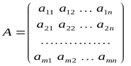
행 및 열 번호 매기기는 배열과 유사하게 0부터 시작합니다.

double 유형의 데이터를 포함하는 '행렬' 및 '벡터' 유형 외에도 4가지 유형이 더 있으며 각각의 유형은 관련된 데이터 작업을 수행합니다.

matrixf —float요소를 포함하는 행렬
matrixc —복소수 요소를 포함하는 행렬
vectorf — float 요소를 포함하는 벡터
vectorc — 복소수 요소를 포함하는 벡터

이 글을 쓰는 시점에서 matrixc 및 vectorc 유형에 대한 작업은 아직 완료되지 않았으므로 이러한 유형을 내장 메서드에서 사용할 수는 없습니다.

템플릿 함수는 해당 유형 대신 matrix<double>, matrix<float>, vector<double>, vector<float>와 같은 표기법을 지원합니다.

  vectorf       v_f1= {0, 1, 2, 3,};
  vector<float> v_f2=v_f1;
  Print("v_f2 = ", v_f2);

  /*
  v_f2 = [0,1,2,3]
  */

생성 및 초기화

행렬 및 벡터 메서드는 목적에 따라 9가지 범주로 나뉩니다. 행렬과 벡터를 선언하고 초기화하는 방법에는 여러 가지가 있습니다.

가장 간단한 생성 방법은 크기 지정이 없는 선언, 다시 말해 데이터에 대한 메모리 할당이 없는 선언입니다. 여기서는 데이터 유형과 변수 이름을 작성합니다:

  matrix         matrix_a;   // double type matrix
  matrix<double> matrix_a1;  // another way to declare a double matrix, suitable for use in templates
  matrix<float>  matrix_a3;  // float type matrix
  vector         vector_a;   // double type vector
  vector<double> vector_a1;  // another notation to create a double vector
  vector<float>  vector_a3;  // float type vector

그런 다음 생성된 객체의 크기를 변경하고 원하는 값으로 채울 수 있습니다. 이들은 계산 결과를 얻기 위해 내장된 행렬 메서드에서 사용될 수 있습니다.

데이터를 위한 메모리를 할당하지만 초기화는 하지 않는 동안 지정된 크기로 행렬 또는 벡터를 선언할 수 있습니다. 여기에서 변수 이름 뒤에 괄호 안에 크기를 지정합니다.

  matrix         matrix_a(128,128);           // the parameters can be either constants
  matrix<double> matrix_a1(InpRows,InpCols);  // or variables
  matrix<float>  matrix_a3(InpRows,1);        // analogue of a vertical vector
  vector         vector_a(256);
  vector<double> vector_a1(InpSize);
  vector<float>  vector_a3(InpSize+16);       // expression can be used as a parameter

객체를 생성하는 세 번째 방법은 초기화로 선언하는 것입니다. 이 경우 행렬 및 벡터 크기는 중괄호로 표시된 초기화 순서에 따라 결정됩니다.

  matrix         matrix_a={{0.1,0.2,0.3},{0.4,0.5,0.6}};
  matrix<double> matrix_a1=matrix_a;                      // the matrices must be of the same type
  matrix<float>  matrix_a3={{1,2},{3,4}};
  vector         vector_a={-5,-4,-3,-2,-1,0,1,2,3,4,5};
  vector<double> vector_a1={1,5,2.4,3.3};
  vector<float>  vector_a3=vector_a2;                     // the vectors must be of the same type

특정 방식으로 초기화된 지정된 크기의 행렬과 벡터를 생성하기 위한 정적 메서드도 있습니다.

  matrix         matrix_a =matrix::Eye(4,5,1);
  matrix<double> matrix_a1=matrix::Full(3,4,M_PI);
  matrixf        matrix_a2=matrixf::Identity(5,5);
  matrixf<float> matrix_a3=matrixf::Ones(5,5);
  matrix         matrix_a4=matrix::Tri(4,5,-1);
  vector         vector_a =vector::Ones(256);
  vectorf        vector_a1=vector<float>::Zeros(16);
  vector<float>  vector_a2=vectorf::Full(128,float_value);

또한 주어진 값(Init및Fill)으로 행렬 또는 벡터를 초기화하는 비 정적인 방법이 있습니다.

  matrix m(2, 2);
  m.Fill(10);
  Print("matrix m \n", m);
  /*
  matrix m
  [[10,10]
  [10,10]]
  */
  m.Init(4, 6);
  Print("matrix m \n", m);
  /*
  matrix m
  [[10,10,10,10,0.0078125,32.00000762939453]
  [0,0,0,0,0,0]
  [0,0,0,0,0,0]
  [0,0,0,0,0,0]]
  */

이 예에서는 Init 메서드를 사용하여 이미 초기화된 행렬의 크기를 변경했는데 이로 인해 모든 새로운 요소가 임의의 값으로 채워졌습니다.

Init 메서드의 중요한 이점은 이 규칙에 따라 행렬/벡터 요소를 채우기 위해 매개변수에 초기화 기능을 지정할수 있다는 것입니다. 예를 들어:

void OnStart()
 {
//---
  matrix init(3, 6, MatrixSetValues);  
  Print("init = \n", init);
  /*
  Execution result
  init = 
  [[1,2,4,8,16,32]
   [64,128,256,512,1024,2048]
   [4096,8192,16384,32768,65536,131072]]
  */   
 }
//+------------------------------------------------------------------+
//| Fills the matrix with powers of a number                         |
//+------------------------------------------------------------------+
void MatrixSetValues(matrix& m, double initial=1)
 {
  double value=initial;
  for(ulong r=0; r<m.Rows(); r++)
   {
    for(ulong c=0; c<m.Cols(); c++)
     {
      m[r][c]=value;
      value*=2;
     }
   }
 }

행렬 및 배열 복사

Copy메서드를 사용하여 행렬과 벡터를 복사할 수 있습니다. 그러나 이러한 데이터 유형을 복사하는 더 간단하고 친숙한 방법은 할당 연산자 "="를 사용하는 것입니다. 또한 복사를 하기 위해 할당 메서드를 사용할 수 있습니다.

//--- copying matrices
  matrix a= {{2, 2}, {3, 3}, {4, 4}};
  matrix b=a+2;
  matrix c;
  Print("matrix a \n", a);
  Print("matrix b \n", b);
  c.Assign(b);
  Print("matrix c \n", c);
  /*
   matrix a
   [[2,2]
    [3,3]
    [4,4]]
   matrix b
   [[4,4]
    [5,5]
    [6,6]]
   matrix c
   [[4,4]
    [5,5]
    [6,6]]
  */

Assign from Copy의 차이점은 행렬과 배열 모두에 사용할 수 있다는 것입니다. 아래 예는 정수 배열int_arr을 이중 행렬로 복사하는 것을 보여줍니다. 결과로 나온 행렬은 복사된 배열의 크기에 따라 자동으로 조정됩니다.

//--- copying an array to a matrix
  matrix double_matrix=matrix::Full(2,10,3.14);
  Print("double_matrix before Assign() \n", double_matrix);
  int int_arr[5][5]= {{1, 2}, {3, 4}, {5, 6}};
  Print("int_arr: ");
  ArrayPrint(int_arr);
  double_matrix.Assign(int_arr);
  Print("double_matrix after Assign(int_arr) \n", double_matrix);  
  /*
   double_matrix before Assign() 
   [[3.14,3.14,3.14,3.14,3.14,3.14,3.14,3.14,3.14,3.14]
    [3.14,3.14,3.14,3.14,3.14,3.14,3.14,3.14,3.14,3.14]]
    
   int_arr: 
       [,0][,1][,2][,3][,4]
   [0,]   1   2   0   0   0
   [1,]   3   4   0   0   0
   [2,]   5   6   0   0   0
   [3,]   0   0   0   0   0
   [4,]   0   0   0   0   0
   
   double_matrix after Assign(int_arr) 
   [[1,2,0,0,0]
    [3,4,0,0,0]
    [5,6,0,0,0]
    [0,0,0,0,0]
    [0,0,0,0,0]]
  */
 }

Assign메서드를 사용하면 크기 및 유형 캐스팅을 자동으로 배열에서 행렬로 원활하게 전환할 수 있습니다.

행렬이나 벡터에 시계열 복사

가격 차트 분석은MqlRates구조 배열을 사용한 작업을 의미합니다. MQL5는 이러한 가격 데이터 구조로 작업하기 위한 새로운 메서드를 제공합니다.

CopyRates메서드는MqlRates구조의 히스토리 시리즈를 행렬이나 벡터에 직접 복사합니다. 따라서 시계열 및 지표에 액세스섹션의 함수를 사용하여 필요한 시계열을 관련 배열로 가져오는 것을 피할 수 있습니다. 또한 이들을 행렬이나 벡터로 전송할 필요가 없습니다. CopyRates 메서드를 사용하면 단 한 번의 호출로 행렬이나 벡터로 쿼트를 받을 수 있습니다. 심볼 리스트에 대한 상관 행렬을 계산하는 방법의 예를 살펴보겠습니다: 두 가지 다른 메서드를 사용하여 이러한 값을 계산하고 결과를 비교하겠습니다.

input int             InBars=100;
input ENUM_TIMEFRAMES InTF=PERIOD_H1;
//+------------------------------------------------------------------+
//| Script program start function                                    |
//+------------------------------------------------------------------+
void OnStart()
 {
//--- list of symbols for calculation
  string symbols[]= {"EURUSD", "GBPUSD", "USDJPY", "USDCAD", "USDCHF"};
  int size=ArraySize(symbols);
//--- matrix and vector to receive Close prices
  matrix rates(InBars, size);
  vector close;
  for(int i=0; i<size; i++)
   {
    //--- get Close prices to a vector
    if(close.CopyRates(symbols[i], InTF, COPY_RATES_CLOSE, 1, InBars))
     {
      //--- insert the vector to the timeseries matrix
      rates.Col(close, i);
      PrintFormat("%d. %s: %d Close prices were added to matrix", i+1, symbols[i], close.Size());
      //--- output the first 20 vector values for debugging
      int  digits=(int)SymbolInfoInteger(symbols[i], SYMBOL_DIGITS);
      Print(VectorToString(close, 20, digits));
     }
    else
     {
      Print("vector.CopyRates(%d,COPY_RATES_CLOSE) failed. Error ", symbols[i], GetLastError());
      return;
     }
   }
  /*
  1. EURUSD: 100 Close prices were added to the matrix
  0.99561 0.99550 0.99674 0.99855 0.99695 0.99555 0.99732 1.00305 1.00121   1.069 0.99936   1.027 1.00130 1.00129 1.00123 1.00201 1.00222 1.00111   1.079   1.030  ...
  2. GBPUSD: 100 Close prices were added to the matrix
  1.13733 1.13708 1.13777 1.14045 1.13985 1.13783 1.13945 1.14315 1.14172 1.13974 1.13868 1.14116 1.14239 1.14230 1.14160 1.14281 1.14338 1.14242 1.14147 1.14069  ...
  3. USDJPY: 100 Close prices were added to the matrix
  143.451 143.356 143.310 143.202 143.079 143.294 143.146 142.963 143.039 143.032 143.039 142.957 142.904 142.956 142.920 142.837 142.756 142.928 143.130 143.069  ...
  4. USDCAD: 100 Close prices were added to the matrix
  1.32840 1.32877 1.32838 1.32660 1.32780 1.33068 1.33001 1.32798 1.32730 1.32782 1.32951 1.32868 1.32716 1.32663 1.32629 1.32614 1.32586 1.32578 1.32650 1.32789  ...
  5. USDCHF: 100 Close prices were added to the matrix
  0.96395 0.96440 0.96315 0.96161 0.96197 0.96337 0.96358 0.96228 0.96474 0.96529 0.96529 0.96502 0.96463 0.96429 0.96378 0.96377 0.96314 0.96428 0.96483 0.96509  ...
  */
//--- prepare a matrix of correlations between symbols
  matrix corr_from_vector=matrix::Zeros(size, size);
  Print("Compute pairwise correlation coefficients");
  for(int i=0; i<size; i++)
   {
    for(int k=i; k<size; k++)
     {
      vector v1=rates.Col(i);
      vector v2=rates.Col(k);
      double coeff = v1.CorrCoef(v2);
      PrintFormat("corr(%s,%s) = %.3f", symbols[i], symbols[k], coeff);
      corr_from_vector[i][k]=coeff;
     }
   }
  Print("Correlation matrix on vectors: \n", corr_from_vector);
  /*
  Calculate pairwise correlation coefficients
  corr(EURUSD,EURUSD) = 1.000
  corr(EURUSD,GBPUSD) = 0.974
  corr(EURUSD,USDJPY) = -0.713
  corr(EURUSD,USDCAD) = -0.950
  corr(EURUSD,USDCHF) = -0.397
  corr(GBPUSD,GBPUSD) = 1.000
  corr(GBPUSD,USDJPY) = -0.744
  corr(GBPUSD,USDCAD) = -0.953
  corr(GBPUSD,USDCHF) = -0.362
  corr(USDJPY,USDJPY) = 1.000
  corr(USDJPY,USDCAD) = 0.736
  corr(USDJPY,USDCHF) = 0.083
  corr(USDCAD,USDCAD) = 1.000
  corr(USDCAD,USDCHF) = 0.425
  corr(USDCHF,USDCHF) = 1.000

  Correlation matrix on vectors:
  [[1,0.9736363791537366,-0.7126365191640618,-0.9503129578410202,-0.3968181226230434]
   [0,1,-0.7440448047501974,-0.9525190338388175,-0.3617774666815978]
   [0,0,1,0.7360546499847362,0.08314381248168941]
   [0,0,0,0.9999999999999999,0.4247042496841555]
   [0,0,0,0,1]]
  */
//--- now let's see how a correlation matrix can be calculated in one line
  matrix corr_from_matrix=rates.CorrCoef(false);   // false means that the vectors are in the matrix columns
  Print("Correlation matrix rates.CorrCoef(false): \n", corr_from_matrix.TriU());
//--- compare the resulting matrices to find discrepancies
  Print("How many discrepancy errors between result matrices?");
  ulong errors=corr_from_vector.Compare(corr_from_matrix.TriU(), (float)1e-12);
  Print("corr_from_vector.Compare(corr_from_matrix,1e-12)=", errors);
  /*
  Correlation matrix rates.CorrCoef(false):
  [[1,0.9736363791537366,-0.7126365191640618,-0.9503129578410202,-0.3968181226230434]
   [0,1,-0.7440448047501974,-0.9525190338388175,-0.3617774666815978]
   [0,0,1,0.7360546499847362,0.08314381248168941]
   [0,0,0,1,0.4247042496841555]
   [0,0,0,0,1]]

  How many discrepancy errors between result matrices?
  corr_from_vector.Compare(corr_from_matrix,1e-12)=0
  */
//--- create a nice output of the correlation matrix
  Print("Output the correlation matrix with headers");
  string header="        ";  // header
  for(int i=0; i<size; i++)
    header+="  "+symbols[i];
  Print(header);
//--- now rows
  for(int i=0; i<size; i++)
   {
    string line=symbols[i]+"  ";
    line+=VectorToString(corr_from_vector.Row(i), size, 3, 8);
    Print(line);
   }
  /*
  Output the correlation matrix with headers
            EURUSD  GBPUSD  USDJPY  USDCAD  USDCHF
  EURUSD       1.0   0.974  -0.713  -0.950  -0.397
  GBPUSD       0.0     1.0  -0.744  -0.953  -0.362
  USDJPY       0.0     0.0     1.0   0.736   0.083
  USDCAD       0.0     0.0     0.0     1.0   0.425
  USDCHF       0.0     0.0     0.0     0.0     1.0
  */
 }
//+------------------------------------------------------------------+
//| Returns a string with vector values                              |
//+------------------------------------------------------------------+
string VectorToString(const vector &v, int length=20, int digits=5, int width=8)
 {
  ulong size=(ulong)MathMin(20, v.Size());
//--- compose a string
  string line="";
  for(ulong i=0; i<size; i++)
   {
    string value=DoubleToString(v[i], digits);
    StringReplace(value, ".000", ".0");
    line+=Indent(width-StringLen(value))+value;
   }
  //--- add a tail if the vector length exceeds the specified size
  if(v.Size()>size)
    line+="  ...";
//---
  return(line);
 }
//+------------------------------------------------------------------+
//|  Returns a string with the specified number of spaces            |
//+------------------------------------------------------------------+
string Indent(int number)
 {
  string indent="";
  for(int i=0; i<number; i++)
    indent+=" ";
  return(indent);
 }

이 예에서는 다음과 같은 내용을 수행하는 방법을 보여줍니다:

CopyRates를 사용하여 종가 가져오기
Col메서드를 사용하여 행렬에 벡터 삽입
CorrCoef를 사용하여 두 벡터 간의 상관 계수 계산
CorrCoef를 사용하여 값 벡터가 있는 행렬에 대한 상관 행렬 계산
TriU메서드를 사용하여 상부 삼각 행렬 반환
두 행렬을 비교하고 Compare 를 사용하여 불일치 찾기

행렬 및 벡터 연산

덧셈, 뺄셈, 곱셈 및 나눗셈의 요소별 수학적 연산이 행렬과 벡터에서 가능합니다. 이러한 작업에서 두 객체는 유형이 같아야 하고 크기가 같아야 합니다. 행렬 또는 벡터의 각 요소는 두 번째 행렬 또는 벡터의 해당 요소에서 작동합니다.

적절한 유형의 스칼라(double, float or complex)를 두 번째 항(승수, 빼기 또는 제수)으로 사용할 수도 있습니다. 이 경우에 행렬 또는 벡터의 각 멤버는 지정된 스칼라에서 작동합니다.

  matrix matrix_a={{0.1,0.2,0.3},{0.4,0.5,0.6}};
  matrix matrix_b={{1,2,3},{4,5,6}};
  matrix matrix_c1=matrix_a+matrix_b;
  matrix matrix_c2=matrix_b-matrix_a;
  matrix matrix_c3=matrix_a*matrix_b;   // Hadamard product
  matrix matrix_c4=matrix_b/matrix_a;
  matrix_c1=matrix_a+1;
  matrix_c2=matrix_b-double_value;
  matrix_c3=matrix_a*M_PI;
  matrix_c4=matrix_b/0.1;
//--- operations in place are possible
  matrix_a+=matrix_b;
  matrix_a/=2;

또한, 행렬 및 벡터는 MathAbs, MathArccos, MathArcsin, MathArctan, MathCeil, MathCos, MathExp, MathFloor, MathLog, MathLog10, MathMod, MathPow, MathRound, MathSin, MathSqrt, MathExpm1, MathLog1p, MathArccosh, MathArcsinh, MathArctanh, MathCosh, MathSinh, MathTanh을 포함한 대부분의 수학 함수에 두 번째 매개변수로 전달할 수 있습니다. 이러한 연산은 행렬과 벡터의 요소별 처리를 의미합니다. 예시:

//---
  matrix a= {{1, 4}, {9, 16}};
  Print("matrix a=\n",a);
  a=MathSqrt(a);
  Print("MatrSqrt(a)=\n",a);
  /*
   matrix a=
   [[1,4]
    [9,16]]
   MatrSqrt(a)=
   [[1,2]
    [3,4]]
  */

MathMod나 MathPow의 경우 두 번째 요소는 스칼라 또는 적절한 크기의 행렬/벡터일 수 있습니다.

   matrix<T> mat1(128,128);
   matrix<T> mat3(mat1.Rows(),mat1.Cols());
   ulong     n,size=mat1.Rows()*mat1.Cols();
...
   mat2=MathPow(mat1,(T)1.9);
   for(n=0; n<size; n++)
     {
      T res=MathPow(mat1.Flat(n),(T)1.9);
      if(res!=mat2.Flat(n))
         errors++;
     }

   mat2=MathPow(mat1,mat3);
   for(n=0; n<size; n++)
     {
      T res=MathPow(mat1.Flat(n),mat3.Flat(n));
      if(res!=mat2.Flat(n))
         errors++;
     }
...
   vector<T> vec1(16384);
   vector<T> vec3(vec1.Size());
   ulong     n,size=vec1.Size();
...
   vec2=MathPow(vec1,(T)1.9);
   for(n=0; n<size; n++)
     {
      T res=MathPow(vec1[n],(T)1.9);
      if(res!=vec2[n])
         errors++;
     }
   vec2=MathPow(vec1,vec3);
   for(n=0; n<size; n++)
     {
      T res=MathPow(vec1[n],vec3[n]);
      if(res!=vec2[n])
         errors++;
     }

조작

MQL5는 계산이 필요 없는 행렬 및 벡터에 대해 다음과 같은 기본 조작을 지원합니다.

전치
행, 열 및 대각선 추출
행렬 크기 조정 및 모양 변경
지정된 행과 열을 교환
새 객체에 복사
두 객체 비교
행렬을 여러개의 부분행렬로 분할
정렬

다음 예제에서는Transpose메서드를 사용하는 행렬 전치를 보여줍니다.

  matrix a= {{0, 1, 2}, {3, 4, 5}};
  Print("matrix a \n", a);
  Print("a.Transpose() \n", a.Transpose());
  /*
  matrix a
  [[0,1,2]
   [3,4,5]]
  a.Transpose()
  [[0,3]
   [1,4]
   [2,5]]
  */

다음은 Diag메서드를 사용하여 대각선을 설정하고 추출하는 방법을 보여주는 예입니다.

   vector v1={1,2,3};
   matrix m1;
   m1.Diag(v1);
   Print("m1\n",m1);
  /* 
  m1
  [[1,0,0]
  [0,2,0]
  [0,0,3]]
  m2
  */

   matrix m2;
   m2.Diag(v1,-1);
   Print("m2\n",m2);
  /*
  m2
  [[0,0,0]
  [1,0,0]
  [0,2,0]
  [0,0,3]]
  */

   matrix m3;
   m3.Diag(v1,1);
   Print("m3\n",m3);
  /*
  m3
  [[0,1,0,0]
  [0,0,2,0]
  [0,0,0,3]]
  */

   matrix m4=matrix::Full(4,5,9);
   m4.Diag(v1,1);
   Print("m4\n",m4);
   
   Print("diag -1 - ",m4.Diag(-1));
   Print("diag 0 - ",m4.Diag());
   Print("diag 1 - ",m4.Diag(1)); 
  /*
  m4
  [[9,1,9,9,9]
  [9,9,2,9,9]
  [9,9,9,3,9]
  [9,9,9,9,9]]
  diag -1 - [9,9,9]
  diag 0 - [9,9,9,9]
  diag 1 - [1,2,3,9]
  */

Reshape 메서드를 사용하여 행렬 크기 변경:

   matrix matrix_a={{1,2,3},{4,5,6},{7,8,9},{10,11,12}};
   Print("matrix_a\n",matrix_a);
  /*
  matrix_a
  [[1,2,3]
   [4,5,6]
   [7,8,9]
   [10,11,12]]

  */

   matrix_a.Reshape(2,6);
   Print("Reshape(2,6)\n",matrix_a);
  /*
  Reshape(2,6)
  [[1,2,3,4,5,6]
   [7,8,9,10,11,12]]
  */

   matrix_a.Reshape(3,5);
   Print("Reshape(3,5)\n",matrix_a);
  /*
  Reshape(3,5)
  [[1,2,3,4,5]
   [6,7,8,9,10]
   [11,12,0,3,0]]
  */

   matrix_a.Reshape(2,4);
   Print("Reshape(2,4)\n",matrix_a);
  /*
  Reshape(2,4)
  [[1,2,3,4]
   [5,6,7,8]]
  */

Vsplit 메서드를 사용한 행렬의 수직 분할 예:

   matrix matrix_a={{ 1, 2, 3, 4, 5, 6},
                    { 7, 8, 9,10,11,12},
                    {13,14,15,16,17,18}};
   matrix splitted[];
   ulong  parts[]={2,3};
 
   matrix_a.Vsplit(2,splitted);
   for(uint i=0; i<splitted.Size(); i++)
      Print("splitted ",i,"\n",splitted[i]);
  /*
     splitted 0
     [[1,2,3]
      [7,8,9]
      [13,14,15]]
     splitted 1
     [[4,5,6]
      [10,11,12]
      [16,17,18]]
  */
 
   matrix_a.Vsplit(3,splitted);
   for(uint i=0; i<splitted.Size(); i++)
      Print("splitted ",i,"\n",splitted[i]);
  /* 
     splitted 0
     [[1,2]
      [7,8]
      [13,14]]
     splitted 1
     [[3,4]
      [9,10]
      [15,16]]
     splitted 2
     [[5,6]
      [11,12]
      [17,18]]
*/
 
   matrix_a.Vsplit(parts,splitted);
   for(uint i=0; i<splitted.Size(); i++)
      Print("splitted ",i,"\n",splitted[i]);
  /* 
     splitted 0
     [[1,2]
      [7,8]
      [13,14]]
     splitted 1
     [[3,4,5]
      [9,10,11]
      [15,16,17]]
     splitted 2
     [[6]
      [12]
      [18]]
  */

Col및Row메서드를 사용하면 관련 행렬 요소를 얻을 수 있을 뿐만 아니라 할당되지 않은 행렬, 즉 지정된 크기가 없는 행렬에 요소를 삽입할 수 있습니다. 다음은 그 예입니다.

   vector v1={1,2,3};
   matrix m1;
   m1.Col(v1,1);
   Print("m1\n",m1);
  /*
   m1
   [[0,1]
    [0,2]
    [0,3]]
  */

   matrix m2=matrix::Full(4,5,8);
   m2.Col(v1,2);
   Print("m2\n",m2);
  /*
   m2
   [[8,8,1,8,8]
    [8,8,2,8,8]

    [8,8,3,8,8]
    [8,8,8,8,8]]   
  */

   Print("col 1 - ",m2.Col(1));
  /*
   col 1 - [8,8,8,8]
  */

   Print("col 2 - ",m2.Col(2));
  /*
   col 1 - [8,8,8,8]  col 2 - [1,2,3,8]
  */

곱

행렬 곱셈은 수치 메서드에서 널리 사용되는 기본 알고리즘 중 하나입니다. 신경망 컨벌루션 계층에서 정방향 및 역방향 전파 알고리즘의 많은 구현이 이 작업을 기반으로 합니다. 종종 머신러닝에 소요되는 전체 시간의 90-95%가 이 작업에 사용됩니다. 모든 곱 메서드는 언어 참조의 행렬 및 벡터의 곱 섹션에서 제공됩니다.

다음 예제는MatMul메서드를 사용한 두 행렬의 곱을 보여줍니다:

   matrix a={{1, 0, 0},
             {0, 1, 0}};
   matrix b={{4, 1},
             {2, 2},
             {1, 3}};
   matrix c1=a.MatMul(b);
   matrix c2=b.MatMul(a);
   Print("c1 = \n", c1);
   Print("c2 = \n", c2);
/*
   c1 = 
   [[4,1]
    [2,2]]
   c2 = 
   [[4,1,0]
    [2,2,0]
    [1,3,0]]
*/

Kron 메서드를 사용하는 두 행렬 또는 행렬과 벡터의 Kronecker 곱의 예입니다.

   matrix a={{1,2,3},{4,5,6}};
   matrix b=matrix::Identity(2,2);
   vector v={1,2};
 
   Print(a.Kron(b));
   Print(a.Kron(v));
 
  /*
   [[1,0,2,0,3,0]
    [0,1,0,2,0,3]
    [4,0,5,0,6,0]
    [0,4,0,5,0,6]]
 
   [[1,2,2,4,3,6]
    [4,8,5,10,6,12]]
  */

MQL5의 행렬 및 벡터 문서에서 더 많은 예를 찾아 볼 수 있습니다:

//--- initialize matrices
   matrix m35, m52;
   m35.Init(3,5,Arange);
   m52.Init(5,2,Arange);
//---
   Print("1. Product of horizontal vector v[3] and matrix m[3,5]");
   vector v3 = {1,2,3};
   Print("On the left v3 = ",v3);
   Print("On the right m35 = \n",m35);
   Print("v3.MatMul(m35) = horizontal vector v[5] \n",v3.MatMul(m35));
   /*
   1. Product of horizontal vector v[3] and matrix m[3,5]
   On the left v3 = [1,2,3]
   On the right m35 =
   [[0,1,2,3,4]
    [5,6,7,8,9]
    [10,11,12,13,14]]
   v3.MatMul(m35) = horizontal vector v[5]
   [40,46,52,58,64]
   */

//--- show that this is really a horizontal vector
   Print("\n2. Product of matrix m[1,3] and matrix m[3,5]");
   matrix m13;
   m13.Init(1,3,Arange,1);
   Print("On the left m13 = \n",m13);
   Print("On the right m35 = \n",m35);
   Print("m13.MatMul(m35) = matrix m[1,5] \n",m13.MatMul(m35));
   /*
   2. Product of matrix m[1,3] and matrix m[3,5]
   On the left m13 =
   [[1,2,3]]
   On the right m35 =
   [[0,1,2,3,4]
    [5,6,7,8,9]
    [10,11,12,13,14]]
   m13.MatMul(m35) = matrix m[1,5]
   [[40,46,52,58,64]]
   */

   Print("\n3. Product of matrix m[3,5] and vertical vector v[5]");
   vector v5 = {1,2,3,4,5};
   Print("On the left m35 = \n",m35);
   Print("On the right v5 = ",v5);
   Print("m35.MatMul(v5) = vertical vector v[3] \n",m35.MatMul(v5));
   /*
   3. Product of matrix m[3,5] and vertical vector v[5]
   On the left m35 =
   [[0,1,2,3,4]
    [5,6,7,8,9]
    [10,11,12,13,14]]
   On the right v5 = [1,2,3,4,5]
   m35.MatMul(v5) = vertical vector v[3]
   [40,115,190]
   */

//--- show that this is really a vertical vector
   Print("\n4. Product of matrix m[3,5] and matrix m[5,1]");
   matrix m51;
   m51.Init(5,1,Arange,1);
   Print("On the left m35 = \n",m35);
   Print("On the right m51 = \n",m51);
   Print("m35.MatMul(m51) = matrix v[3] \n",m35.MatMul(m51));
   /*
   4. Product of matrix m[3,5] and matrix m[5,1]
   On the left m35 =
   [[0,1,2,3,4]
    [5,6,7,8,9]
    [10,11,12,13,14]]
   On the right m51 =
   [[1]
    [2]
    [3]
    [4]
    [5]]
   m35.MatMul(m51) = matrix v[3]
   [[40]
    [115]
    [190]]
   */

   Print("\n5. Product of matrix m[3,5] and matrix m[5,2]");
   Print("On the left m35 = \n",m35);
   Print("On the right m52 = \n",m52);
   Print("m35.MatMul(m52) = matrix m[3,2] \n",m35.MatMul(m52));
   /*
   5. Product of matrix m[3,5] and matrix m[5,2]
   On the left m35 =
   [[0,1,2,3,4]
    [5,6,7,8,9]
    [10,11,12,13,14]]
   On the right m52 =
   [[0,1]
    [2,3]
    [4,5]
    [6,7]
    [8,9]]
   m35.MatMul(m52) = matrix m[3,2]
   [[60,70]
    [160,195]
    [260,320]]
   */

   Print("\n6. Product of horizontal vector v[5] and matrix m[5,2]");
   Print("On the left v5 = \n",v5);
   Print("On the right m52 = \n",m52);
   Print("v5.MatMul(m52) = horizontal vector v[2] \n",v5.MatMul(m52));
   /*
   6. The product of horizontal vector v[5] and matrix m[5,2]
   On the left v5 =
   [1,2,3,4,5]
   On the right m52 =
   [[0,1]
    [2,3]
    [4,5]
    [6,7]
    [8,9]]
   v5.MatMul(m52) = horizontal vector v[2]
   [80,95]
   */

   Print("\n7. Outer() product of horizontal vector v[5] and vertical vector v[3]");
   Print("On the left v5 = \n",v5);
   Print("On the right v3 = \n",v3);
   Print("v5.Outer(v3) = matrix m[5,3] \n",v5.Outer(v3));
   /*
   7. Outer() product of horizontal vector v[5] and vertical vector v[3]
   On the left v5 =
   [1,2,3,4,5]
   On the right v3 =
   [1,2,3]
   v5.Outer(v3) = matrix m[5,3]
   [[1,2,3]
    [2,4,6]
    [3,6,9]
    [4,8,12]
    [5,10,15]]
   */

변환

행렬 변환은 종종 데이터 작업에 사용됩니다. 그러나 많은 복잡한 행렬 연산은 컴퓨터의 제한된 정확도로 인해 효율적으로 풀 수 없거나 안정적으로 풀 수 없습니다.

행렬 변환(또는 분해)은 행렬을 구성 요소로 줄이는 메서드로서 더 복잡한 행렬 연산을 더 쉽게 계산할 수 있도록 해 줍니다. 행렬 분해 메서드는 선형 방정식 풀이 시스템, 역행렬 계산, 행렬의 행렬식 계산과 같은 기본 연산에서도 컴퓨터 선형 대수의 근간입니다.

머신 러닝은 SVD(Singular Value Decomposition)를 널리 사용하므로 원래 행렬을 다른 3개 행렬의 곱으로 표현할 수 있습니다. SVD는 최소 제곱법 근사에서 압축 및 이미지 인식에 이르기까지 다양한 문제를 해결하는 데 사용됩니다.

SVD방법에 의한 특이값 분해의 예:

  matrix a= {{0, 1, 2, 3, 4, 5, 6, 7, 8}};
  a=a-4;
  Print("matrix a \n", a);
  a.Reshape(3, 3);
  matrix b=a;
  Print("matrix b \n", b);
//--- execute SVD decomposition
  matrix U, V;
  vector singular_values;
  b.SVD(U, V, singular_values);
  Print("U \n", U);
  Print("V \n", V);
  Print("singular_values = ", singular_values);
 
// check block
//--- U * singular diagonal * V = A
  matrix matrix_s;
  matrix_s.Diag(singular_values);
  Print("matrix_s \n", matrix_s);
  matrix matrix_vt=V.Transpose();
  Print("matrix_vt \n", matrix_vt);
  matrix matrix_usvt=(U.MatMul(matrix_s)).MatMul(matrix_vt);
  Print("matrix_usvt \n", matrix_usvt);
 
  ulong errors=(int)b.Compare(matrix_usvt, 1e-9);
  double res=(errors==0);
  Print("errors=", errors);
 
//---- another check
  matrix U_Ut=U.MatMul(U.Transpose());
  Print("U_Ut \n", U_Ut);
  Print("Ut_U \n", (U.Transpose()).MatMul(U));
 
  matrix vt_V=matrix_vt.MatMul(V);
  Print("vt_V \n", vt_V);
  Print("V_vt \n", V.MatMul(matrix_vt)); 
  /*
  matrix a
  [[-4,-3,-2,-1,0,1,2,3,4]]
  matrix b
  [[-4,-3,-2]
   [-1,0,1]
   [2,3,4]]
  U
  [[-0.7071067811865474,0.5773502691896254,0.408248290463863]
   [-6.827109697437648e-17,0.5773502691896253,-0.8164965809277256]
   [0.7071067811865472,0.5773502691896255,0.4082482904638627]]
  V
  [[0.5773502691896258,-0.7071067811865474,-0.408248290463863]
   [0.5773502691896258,1.779939029415334e-16,0.8164965809277258]
   [0.5773502691896256,0.7071067811865474,-0.408248290463863]]
  singular_values = [7.348469228349533,2.449489742783175,3.277709923350408e-17]
 
  matrix_s
  [[7.348469228349533,0,0]
   [0,2.449489742783175,0]
   [0,0,3.277709923350408e-17]]
  matrix_vt
  [[0.5773502691896258,0.5773502691896258,0.5773502691896256]
   [-0.7071067811865474,1.779939029415334e-16,0.7071067811865474]
   [-0.408248290463863,0.8164965809277258,-0.408248290463863]]
  matrix_usvt
  [[-3.999999999999997,-2.999999999999999,-2]
   [-0.9999999999999981,-5.977974170712231e-17,0.9999999999999974]
   [2,2.999999999999999,3.999999999999996]]
  errors=0
 
  U_Ut
  [[0.9999999999999993,-1.665334536937735e-16,-1.665334536937735e-16]
   [-1.665334536937735e-16,0.9999999999999987,-5.551115123125783e-17]
   [-1.665334536937735e-16,-5.551115123125783e-17,0.999999999999999]]
  Ut_U
  [[0.9999999999999993,-5.551115123125783e-17,-1.110223024625157e-16]
   [-5.551115123125783e-17,0.9999999999999987,2.498001805406602e-16]
   [-1.110223024625157e-16,2.498001805406602e-16,0.999999999999999]]
  vt_V
  [[1,-5.551115123125783e-17,0]
   [-5.551115123125783e-17,0.9999999999999996,1.110223024625157e-16]
   [0,1.110223024625157e-16,0.9999999999999996]]
  V_vt
  [[0.9999999999999999,1.110223024625157e-16,1.942890293094024e-16]
   [1.110223024625157e-16,0.9999999999999998,1.665334536937735e-16]
   [1.942890293094024e-16,1.665334536937735e-16,0.9999999999999996]
  */
 }

일반적으로 사용되는 또 다른 변환은 행렬 A가 양의 정부호 행렬인 경우 선형 방정식 시스템 Ax=b를 푸는 데 사용할 수 있는 촐레스키 분해입니다.

MQL5에서 촐레스키 분해는Cholesky메서드로 실행됩니다.

  matrix matrix_a= {{5.7998084, -2.1825367}, {-2.1825367, 9.85910595}};
  matrix matrix_l;
  Print("matrix_a\n", matrix_a);
 
  matrix_a.Cholesky(matrix_l);
  Print("matrix_l\n", matrix_l);
  Print("check\n", matrix_l.MatMul(matrix_l.Transpose()));  
  /*
  matrix_a
  [[5.7998084,-2.1825367]
   [-2.1825367,9.85910595]]
  matrix_l
  [[2.408279136645086,0]
   [-0.9062640068544704,3.006291985133859]]
  check
  [[5.7998084,-2.1825367]
   [-2.1825367,9.85910595]]
  */

아래 표는 사용 가능한 메서드 목록을 보여줍니다.

함수	수행 동작
Cholesky	촐레스키 분해를 계산합니다.
Eig	정방 행렬의 고유값과 오른쪽 고유 벡터를 계산합니다.
EigVal	일반 행렬의 고유값을 계산합니다.
LU	하부 삼각 행렬과 상부 삼각 행렬의 곱으로 행렬의 LU 분해
LUP	행 순열만 있는 LU 분해를 참조하는 부분 피벗을 사용한 LUP 분해: PA=LU
QR	행렬의 qr 분해 계산
SVD	특이값 분해

통계 얻기

통계 섹션의 메서드는 행렬 및 벡터의 기술 통계를 계산하는 데 사용됩니다. 다음을 찾는 데 사용하십시오:

행렬/벡터의 인덱스와 함께 최대값 및 최소값
요소의 합과 곱, 누적 합과 곱
행렬/벡터 값의 중앙값, 평균, 산술 평균 및 가중 산술 평균
표준 편차 및 요소 분산
백분위수 및 분위수
지정된 데이터 배열에 구성된 회귀선과의 편차 오차로서의 회귀 메트릭

Std 메서드로 표준 편차를 계산하는 예:

   matrixf matrix_a={{10,3,2},{1,8,12},{6,5,4},{7,11,9}};
   Print("matrix_a\n",matrix_a);
 
   vectorf cols_std=matrix_a.Std(0);
   vectorf rows_std=matrix_a.Std(1);
   float matrix_std=matrix_a.Std();
 
   Print("cols_std ",cols_std);
   Print("rows_std ",rows_std);
   Print("std value  ",matrix_std);
   /*
   matrix_a
   [[10,3,2]
    [1,8,12]
    [6,5,4]
    [7,11,9]]
   cols_std [3.2403703,3.0310888,3.9607449]
   rows_std [3.5590262,4.5460606,0.81649661,1.6329932]
   std value  3.452052593231201
   */

Quantile 메서드로 Quantile 계산:

   matrixf matrix_a={{1,2,3},{4,5,6},{7,8,9},{10,11,12}};
   Print("matrix_a\n",matrix_a);
 
   vectorf cols_percentile=matrix_a.Percentile(50,0);
   vectorf rows_percentile=matrix_a.Percentile(50,1);
   float matrix_percentile=matrix_a.Percentile(50);
 
   Print("cols_percentile ",cols_percentile);
   Print("rows_percentile ",rows_percentile);
   Print("percentile value  ",matrix_percentile);
   /*
   matrix_a
   [[1,2,3]
    [4,5,6]
    [7,8,9]
    [10,11,12]]
   cols_percentile [5.5,6.5,7.5]
   rows_percentile [2,5,8,11]
   percentile value  6.5
   */

매트릭스 특성

특성 섹션의 메서드를 사용하여 다음 값을 얻습니다.

행렬의 행 수와 열 수
규범 및 조건 번호
행렬의 행렬식, 순위, 추적 및 스펙트럼

Rank 메서드를 사용하여 행렬의 순위 계산:

  matrix a=matrix::Eye(4, 4);;
  Print("matrix a \n", a);
  Print("a.Rank()=", a.Rank());
 
  matrix I=matrix::Eye(4, 4);
  I[3, 3] = 0.;    // matrix deficit
  Print("I \n", I);
  Print("I.Rank()=", I.Rank());
 
  matrix b=matrix::Ones(1, 4);
  Print("b \n", b);
  Print("b.Rank()=", b.Rank());;// 1 size - rank 1, unless all 0
 
  matrix  zeros=matrix::Zeros(4, 1);
  Print("zeros \n", zeros);
  Print("zeros.Rank()=", zeros.Rank()); 
  /*
  matrix a
  [[1,0,0,0]
  [0,1,0,0]
  [0,0,1,0]
  [0,0,0,1]]
  a.Rank()=4
 
  I
  [[1,0,0,0]
  [0,1,0,0]
  [0,0,1,0]
  [0,0,0,0]]
  I.Rank()=3
 
  b
  [[1,1,1,1]]
  b.Rank()=1
 
  zeros
  [[0]
  [0]
  [0]
  [0]]
  zeros.Rank()=0
  */

Norm 메서드를 사용하여 규범 계산:

  matrix a= {{0, 1, 2, 3, 4, 5, 6, 7, 8}};
  a=a-4;
  Print("matrix a \n", a);
  a.Reshape(3, 3);
  matrix b=a;
  Print("matrix b \n", b);
  Print("b.Norm(MATRIX_NORM_P2)=", b.Norm(MATRIX_NORM_FROBENIUS));
  Print("b.Norm(MATRIX_NORM_FROBENIUS)=", b.Norm(MATRIX_NORM_FROBENIUS));
  Print("b.Norm(MATRIX_NORM_INF)", b.Norm(MATRIX_NORM_INF));
  Print("b.Norm(MATRIX_NORM_MINUS_INF)", b.Norm(MATRIX_NORM_MINUS_INF));
  Print("b.Norm(MATRIX_NORM_P1)=)", b.Norm(MATRIX_NORM_P1));
  Print("b.Norm(MATRIX_NORM_MINUS_P1)=", b.Norm(MATRIX_NORM_MINUS_P1));
  Print("b.Norm(MATRIX_NORM_P2)=", b.Norm(MATRIX_NORM_P2));
  Print("b.Norm(MATRIX_NORM_MINUS_P2)=", b.Norm(MATRIX_NORM_MINUS_P2)); 
  /*
  matrix a
  [[-4,-3,-2,-1,0,1,2,3,4]]
  matrix b
  [[-4,-3,-2]
  [-1,0,1]
  [2,3,4]]
  b.Norm(MATRIX_NORM_P2)=7.745966692414834
  b.Norm(MATRIX_NORM_FROBENIUS)=7.745966692414834
  b.Norm(MATRIX_NORM_INF)9.0
  b.Norm(MATRIX_NORM_MINUS_INF)2.0
  b.Norm(MATRIX_NORM_P1)=)7.0
  b.Norm(MATRIX_NORM_MINUS_P1)=6.0
  b.Norm(MATRIX_NORM_P2)=7.348469228349533
  b.Norm(MATRIX_NORM_MINUS_P2)=1.857033188519056e-16
  */

방정식 풀기

머신러닝 메서드 및 최적화 문제는 종종 선형 방정식 시스템에 대한 솔루션을 찾을 것을 요구합니다. 솔루션 섹션에는 행렬 유형에 따라 이러한 방정식의 솔루션을 허용하는 네개의 메서드가 포함되어 있습니다.

함수	수행 동작
Solve	선형 행렬 방정식 또는 선형 대수 방정식 시스템 풀기
LstSq	선형 대수 방정식의 최소 제곱 해를 반환합니다(비제곱 또는 degenerate matrices의 경우).
Inv	Jordan-Gauss 메서드로 가역 정방 행렬의 곱셈의 역을 계산합니다.
PINV	무어-펜로즈 메서드로 행렬의 의사 역행렬 계산

방정식 A*x=b를 푸는 예를 보십시오.

우리는 솔루션 벡터 x를 찾아야 합니다. 행렬 A는 정사각형이 아니므로 여기에서Solve 메서드를 사용할 수 없습니다.

우리는 non-sqaure 또는 degenerate 행렬의 대략적인 풀이를 가능하게 하는 LstSq메서드를 사용할 것입니다.

   matrix a={{3, 2},
             {4,-5},
             {3, 3}};
   vector b={7,40,3};
//--- solve the system A*x = b
   vector x=a.LstSq(b);
//--- check the solution, x must be equal to [5, -4]
   Print("x=", x);
  /*
  x=[5.00000000,-4]
  */

//--- check A*x = b1, the resulting vector must be [7, 40, 3]
   vector b1=a.MatMul(x);
   Print("b11=",b1); 
/*
  b1=[7.0000000,40.0000000,3.00000000]
*/

확인 결과 찾아낸 벡터 x가 이 연립방정식의 해임을 보여주었습니다.

머신러닝 메서드

머신러닝에 사용할 수 있는 세 가지 행렬 및 벡터 메서드가 있습니다.

함수	수행 동작
활성화	활성화 함수 값을 계산하고 계산한 값을 전달된 벡터/행렬에 씁니다.
도함수	활성화 함수 도함수 값을 계산하고 계산된 값을 전달된 벡터/행렬에 씁니다.
손실	손실 함수 값을 계산하고 계산된 값을 전달된 벡터/행렬에 씁니다.

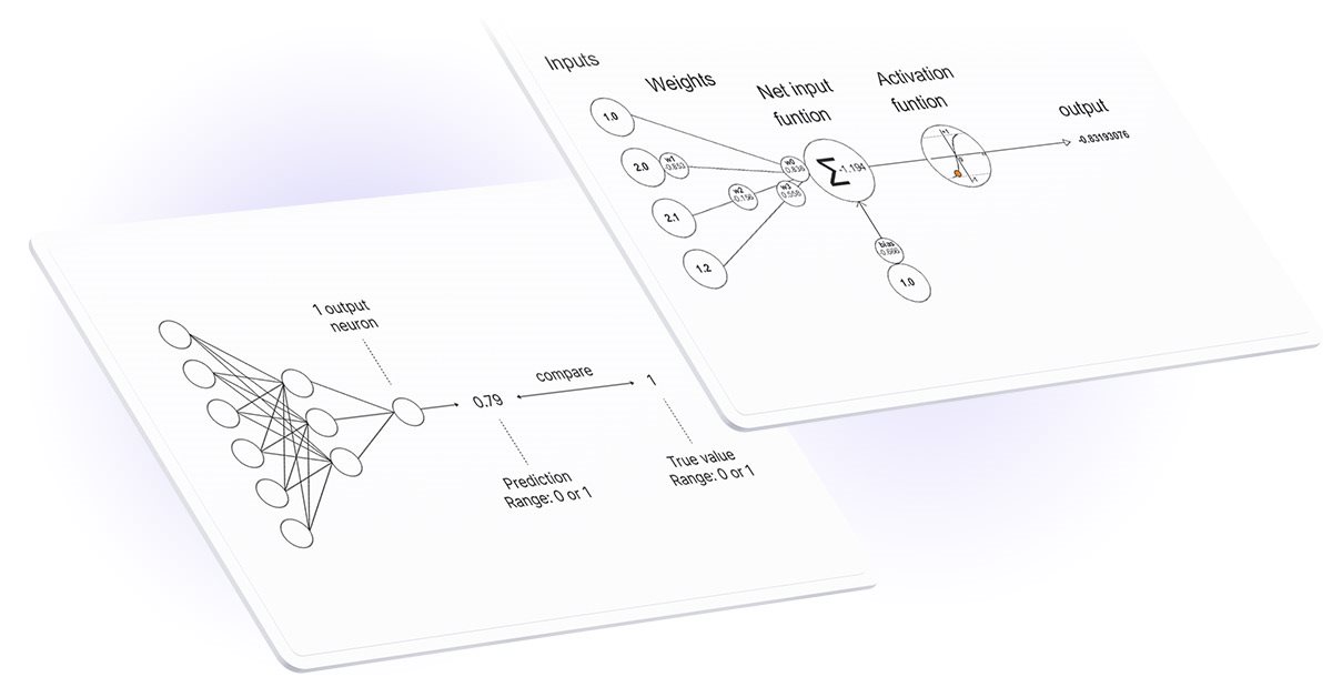
활성화 함수는 신경망에서 입력의 가중치 합에 따라 출력을 찾기 위해 사용됩니다. 활성화 함수의 선택은 신경망의 성능에 큰 영향을 미칩니다.

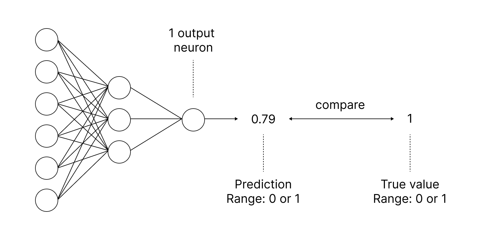
가장 널리 사용되는 활성화 함수 중 하나는 시그모이드입니다.

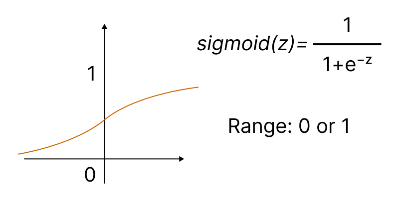
내장된 활성화 메서드를 사용하면 활성화 기능의 15가지 유형 중 하나를 설정할 수 있습니다. 모두ENUM_ACTIVATION_FUNCTION열거형에서 사용할 수 있습니다.

ID	설명
AF_ELU	지수 선형 단위
AF_EXP	지수
AF_GELU	가우스 오차 선형 단위
AF_HARD_SIGMOID	하드 시그모이드
AF_LINEAR	선형
AF_LRELU	Leaky REctified Linear Unit
AF_RELU	REctified Linear Unit
AF_SELU	스케일된 지수 선형 단위
AF_SIGMOID	시그모이드
AF_SOFTMAX	소프트맥스
AF_SOFTPLUS	소프트플러스
AF_SOFTSIGN	소프트사인
AF_SWISH	Swish
AF_TANH	쌍곡선 탄젠트 함수
AF_TRELU	Thresholded REctified Linear Unit

신경망은 학습에서 오류를 최소화하는 알고리즘을 찾는 것을 목표로 하며 이를 위해 손실 함수를 사용합니다. 편차는ENUM_LOSS_FUNCTION열거형에서 14가지 유형 중 하나를 지정할 수 있는 손실 메서드를 사용하여 계산됩니다.

구해진 편차 값은 신경망 매개변수를 수정하는 데 사용됩니다. 이것은 활성화 함수의 도함수 값을 계산하고 그 결과를 전달된 벡터/행렬에 쓰는 도함수 메서드를 사용하여 수행됩니다. 신경망 훈련 과정은 "MQL 언어를 사용하여 처음부터 심층 신경망 프로그래밍 하기"와 같은 기사의 애니메이션을 사용하여 시각적으로 표현할 수 있습니다.

OpenCL의 개선 사항

또한CLBufferWrite및CLBufferRead함수에서 행렬 및 벡터를 지원 하도록 구현했습니다. 이러한 함수들을 위해 해당하는 오버로드를 사용할 수 있습니다. 행렬의 예는 아래와 같습니다.

행렬의 값을 버퍼에 쓰고 성공하면 true를 반환합니다.

uint  CLBufferWrite(
   int           buffer,                    // OpenCL buffer handle
   uint          buffer_offset,             // offset in the OpenCL buffer in bytes
   matrix<T>     &mat                       // matrix of values to write to buffer
   );

OpenCL 버퍼를 행렬로 읽고 성공하면 true를 반환합니다.

uint  CLBufferRead(
   int           buffer,                    // OpenCL buffer handle
   uint          buffer_offset,             // offset in the OpenCL buffer in bytes
   const matrix& mat,                       // matrix to get values from the buffer
   ulong         rows=-1,                   // number of rows in the matrix
   ulong         cols=-1                    // number of columns in the matrix
   );

두 행렬의 행렬 곱의 예를 사용하여 새 오버로드를 사용하는 경우에 대해 알아 보겠습니다. 세 가지의 방법을 사용하여 계산을 수행해 보겠습니다.

행렬 곱셈 알고리즘을 나타내는 단순한 방법
내장된 MatMul메서드
OpenCL의 병렬 계산

구해진 행렬은 주어진 정밀도로 두 행렬의 요소를 비교하는Compare메서드를 사용하여 확인됩니다.

#define M       3000      // number of rows in the first matrix
#define K       2000      // number of columns in the first matrix equal to the number of rows in the second one
#define N       3000      // number of columns in the second matrix
 
//+------------------------------------------------------------------+
const string clSrc=
  "#define N     "+IntegerToString(N)+"                              \r\n"
  "#define K     "+IntegerToString(K)+"                              \r\n"
  "                                                                  \r\n"
  "__kernel void matricesMul( __global float *in1,                   \r\n"
  "                           __global float *in2,                   \r\n"
  "                           __global float *out  )                 \r\n"
  "{                                                                 \r\n"
  "  int m = get_global_id( 0 );                                     \r\n"
  "  int n = get_global_id( 1 );                                     \r\n"
  "  float sum = 0.0;                                                \r\n"
  "  for( int k = 0; k < K; k ++ )                                   \r\n"
  "     sum += in1[ m * K + k ] * in2[ k * N + n ];                  \r\n"
  "  out[ m * N + n ] = sum;                                         \r\n"
  "}                                                                 \r\n";
//+------------------------------------------------------------------+
//| Script program start function                                    |
//+------------------------------------------------------------------+
void OnStart()
 {
//--- initialize the random number generator
  MathSrand((int)TimeCurrent());
//--- fill matrices of the given size with random values
  matrixf mat1(M, K, MatrixRandom) ;    // first matrix
  matrixf mat2(K, N, MatrixRandom);     // second matrix
 
//--- calculate the product of matrices using the naive way
  uint start=GetTickCount();
  matrixf matrix_naive=matrixf::Zeros(M, N);// here we rite the result of multiplying two matrices
  for(int m=0; m<M; m++)
    for(int k=0; k<K; k++)
      for(int n=0; n<N; n++)
        matrix_naive[m][n]+=mat1[m][k]*mat2[k][n];
  uint time_naive=GetTickCount()-start;   
     
//--- calculate the product of matrices using MatMull
  start=GetTickCount();
  matrixf matrix_matmul=mat1.MatMul(mat2);
  uint time_matmul=GetTickCount()-start;     
  
//--- calculate the product of matrices in OpenCL
  matrixf matrix_opencl=matrixf::Zeros(M, N);
  int cl_ctx;             // context handle
  if((cl_ctx=CLContextCreate(CL_USE_GPU_ONLY))==INVALID_HANDLE)
   {
    Print("OpenCL not found, exit");
    return;
   }
  int cl_prg;             // program handle
  int cl_krn;             // kernel handle
  int cl_mem_in1;         // handle of the first buffer (input)
  int cl_mem_in2;         // handle of the second buffer (input)
  int cl_mem_out;         // handle of the third buffer (output)
//--- create the program and the kernel
  cl_prg = CLProgramCreate(cl_ctx, clSrc);
  cl_krn = CLKernelCreate(cl_prg, "matricesMul");
//--- create all three buffers for the three matrices
  cl_mem_in1=CLBufferCreate(cl_ctx, M*K*sizeof(float), CL_MEM_READ_WRITE);
  cl_mem_in2=CLBufferCreate(cl_ctx, K*N*sizeof(float), CL_MEM_READ_WRITE);
//--- third matrix - output
  cl_mem_out=CLBufferCreate(cl_ctx, M*N*sizeof(float), CL_MEM_READ_WRITE);
//--- set kernel arguments
  CLSetKernelArgMem(cl_krn, 0, cl_mem_in1);
  CLSetKernelArgMem(cl_krn, 1, cl_mem_in2);
  CLSetKernelArgMem(cl_krn, 2, cl_mem_out);
//--- write matrices to device buffers
  CLBufferWrite(cl_mem_in1, 0, mat1);
  CLBufferWrite(cl_mem_in2, 0, mat2);
  CLBufferWrite(cl_mem_out, 0, matrix_opencl);
//--- start the OpenCL code execution time
  start=GetTickCount();
//--- set the task workspace parameters and execute the OpenCL program
  uint  offs[2] = {0, 0};
  uint works[2] = {M, N};
  start=GetTickCount();  
  bool ex=CLExecute(cl_krn, 2, offs, works);
//--- read the result into the matrix
  if(CLBufferRead(cl_mem_out, 0, matrix_opencl))
    PrintFormat("Matrix [%d x %d] read ", matrix_opencl.Rows(), matrix_opencl.Cols());
   else
      Print("CLBufferRead(cl_mem_out, 0, matrix_opencl failed. Error ",GetLastError()); 
  uint time_opencl=GetTickCount()-start;   
  Print("Compare computation times of the methods");
  PrintFormat("Naive product time = %d ms",time_naive);
  PrintFormat("MatMul product time = %d ms",time_matmul);
  PrintFormat("OpenCl product time = %d ms",time_opencl);  
//--- release all OpenCL contexts
  CLFreeAll(cl_ctx, cl_prg, cl_krn, cl_mem_in1, cl_mem_in2, cl_mem_out);
 
//--- compare all obtained result matrices with each other 
  Print("How many discrepancy errors between result matrices?");
  ulong errors=matrix_naive.Compare(matrix_matmul,(float)1e-12);
  Print("matrix_direct.Compare(matrix_matmul,1e-12)=",errors);
  errors=matrix_matmul.Compare(matrix_opencl,float(1e-12));
  Print("matrix_matmul.Compare(matrix_opencl,1e-12)=",errors);
/*
   Result: 
   
   Matrix [3000 x 3000] read 
   Compare computation times of the methods
   Naive product time = 54750 ms
   MatMul product time = 4578 ms
   OpenCl product time = 922 ms
   How many discrepancy errors between result matrices?
   matrix_direct.Compare(matrix_matmul,1e-12)=0
   matrix_matmul.Compare(matrix_opencl,1e-12)=0
*/  
 }
//+------------------------------------------------------------------+
//| Fills the matrix with random values                              |
//+------------------------------------------------------------------+
void MatrixRandom(matrixf& m)
 {
  for(ulong r=0; r<m.Rows(); r++)
   {
    for(ulong c=0; c<m.Cols(); c++)
     {
      m[r][c]=(float)((MathRand()-16383.5)/32767.);
     }
   }
 }
//+------------------------------------------------------------------+
//| Release all OpenCL contexts                                      |
//+------------------------------------------------------------------+
void CLFreeAll(int cl_ctx, int cl_prg, int cl_krn,
               int cl_mem_in1, int cl_mem_in2, int cl_mem_out)
 {
//--- release all created OpenCL contexts in reverse order
  CLBufferFree(cl_mem_in1);
  CLBufferFree(cl_mem_in2);
  CLBufferFree(cl_mem_out);
  CLKernelFree(cl_krn);
  CLProgramFree(cl_prg);
  CLContextFree(cl_ctx);
 }

이 예제에서 사용한 OpenCL 코드에 대한 자세한 설명은 다음의 기사에서 확인 할 수 있습니다. "OpenCL: 단순한 것에서 보다 통찰력 있는 코딩으로".

더 많은 개선 사항

빌드 3390은 GPU 사용에 대해 영향을 미치는 OpenCL 작업의 두 가지 제한을 없엤습니다.

OpenCL 객체의 최대 수는 최대 65536개까지 가능하지만 이전에는 256개로 제한되었습니다. OpenCL 객체의 핸들은CLContextCreate,CLBufferCreate와 CLProgramCreate함수를 사용하여 MQL5 프로그램에서 생성됩니다. 예전에는 핸들을 256개로 제한한 나머지 머신 러닝의 메서드를 효율적으로 사용할 수 없었습니다.

OpenCL은 'double'의 지원 없이 그래픽 카드에서 사용될 수 있습니다. 이전에도 많은 작업에서 float를 사용한 계산이 허용되었음에도 불구하고 MQL5 프로그램에서는 Double을 지원하는 GPU만 허용되었습니다. float 유형은 공간을 덜 차지하므로 원론적으로 병렬 컴퓨팅의 기본으로 간주됩니다. 따라서 이전의 요구 사항은 없어졌습니다.

특정 작업에 대해 double을 지원하고 GPU를 필수적으로 사용하는 것으로 설정하려면 CLContextCreate 호출에서 CL_USE_GPU_DOUBLE_ONLY를 사용하십시오.

   int cl_ctx;
//--- initialization of OpenCL context
   if((cl_ctx=CLContextCreate(CL_USE_GPU_DOUBLE_ONLY))==INVALID_HANDLE)
     {
      Print("OpenCL not found");
      return;
     }

OpenCL 수행의 변경 사항은 행렬 및 벡터와 직접적인 관련이 없지만 MQL5 언어의 머신 러닝 기능을 발전시키려는 저희의 노력을 보여줍니다.

머신 러닝과 MQL5의 미래

지난 몇 년 동안 우리는 MQL5 언어에 고급 기술을 도입하기 위해 많은 노력을 기울였습니다.

수와 관련한 메서드의 ALGLIB라이브러리를 MQL5로 포팅
퍼지 논리 및 통계 메서드로 수학 라이브러리구현
plot 함수와 같은 그래픽 라이브러리소개
터미널에서 직접 Python 스크립트를 실행하기 위해 Python과 통합
DirectX 함수를 추가하여 3D 그래픽 생성
데이터베이스 작업을 위한 기본SQLite 지원구현
필요한 모든 메서드와 새로운 데이터 유형 추가: 행렬 및 벡터

MQL5 언어는 계속 발전할 것이며 가장 우선적으로는 머신 러닝과 관련한 것들입니다. 저희는 큰 계획을 가지고 계속적인 발전을 해 나아갈 것입니다. 그러니 저희와 함께 하고 저희를 지원하고 저희와 함께 계속 배우십시오.

MetaQuotes 소프트웨어 사를 통해 러시아어가 번역됨.
원본 기고글: https://www.mql5.com/ru/articles/10922

경고: 이 자료들에 대한 모든 권한은 MetaQuotes(MetaQuotes Ltd.)에 있습니다. 이 자료들의 전부 또는 일부에 대한 복제 및 재출력은 금지됩니다.

이 작가의 다른 글

토론으로 가기

Expert Advisor 개발 기초부터 (파트 12): 시간과 거래(I)

오늘은 주문의 흐름을 알아보기 위해 Times & Trade를 만들 것입니다. 이는 우리가 앞으로 구축할 시스템의 첫 번째 부분입니다. 다음 글에서는 추가적인 내용을 더해 시스템을 완성하도록 하겠습니다. 이 새로운 기능을 구현하려면 Expert Advisor 코드에 몇 가지의 새로운 항목을 추가해야 합니다.

누적/분배(Accumulation/Distribution (AD))에 기반한 거래 시스템을 설계하는 방법

이 글은 가장 인기 있는 기술 지표를 기반으로 거래 시스템을 설계하는 방법에 대한 시리즈의 새로운 글입니다. 이 글에서는 누적/분배 지표라는 새로운 기술 지표에 대해 배우고 간단한 AD 거래 전략을 기반으로 하여 MQL5 거래 시스템을 설계하는 방법에 대해 알아봅니다.

MQL5에서 행렬 및 벡터

특수한 데이터 유형인 '매트릭스' 및 '벡터'를 사용하여 수학적 표기법에 매우 가까운 코드를 생성할 수 있습니다. 이러한 메서드를 사용하면 중첩된 루프를 만들거나 계산시 배열의 올바른 인덱싱을 염두에 둘 필요가 없습니다. 따라서 행렬 및 벡터 메서드를 사용하면 복잡한 프로그램을 개발할 때 안정성과 속도가 향상됩니다.

OBV로 트레이딩 시스템을 설계하는 방법 알아보기

이 기사는 인기있는 지표 중 일부를 기반으로 거래 시스템을 설계하는 방법에 대해 초보자들에게 설명하는 시리즈에서 계속되는 새로운 기사입니다. OBV(On Balance Volume)라는 새로운 지표를 배우고 이를 어떻게 사용하고 이를 기반으로 하는 거래 시스템을 어떻게 설계하는지 알아보겠습니다.