Time Evolution Travel Algorithm (TETA)

Contents

1. Introduction
2. Implementation of the algorithm
3. Test results

Introduction

We have looked at many algorithms based on physical laws, such as CSS, EM, GSA, AEFA, AOSm, however, the universe constantly delights us with new phenomena and fills us with various hypotheses and ideas. One of the fundamental components of the universe, such as time, gave me the idea of creating a new optimization algorithm. Time not only inspires new discoveries, but also remains a mysterious entity that is difficult to comprehend. It flows like a river, carrying away moments of our lives and leaving only memories. Time travel has always been a subject of human fascination and fantasy. To better understand the idea of the algorithm, let's imagine the story of one scientist.

Once upon a time there lived a physicist who was obsessed with the idea of moving to a bright future, away from the mistakes he had made. Having delved into the study of time flows, he was faced with a bitter discovery: travel into the future is impossible. Undeterred, he switched to researching the ability to travel back to the past, hoping to correct his mistakes, but here too he was disappointed.

However, his study of hypothetical time flows led him to a startling discovery: the existence of parallel universes. Having developed a theoretical model of a machine for moving between worlds, he discovered something astonishing: although direct time travel is impossible, it is possible to choose a sequence of events leading to one or another parallel universe.

Every action of any person gave birth to a new parallel reality, but the scientist was only interested in those universes that directly affected his life. To navigate between them, he established special anchors in the system of equations (to distinguish between the worlds) - key points of his destiny: family, career, scientific discoveries, friendships and significant events. These anchors became variables in his machine, allowing him to choose the optimal path between probabilistic worlds.

Having launched his invention, he began a journey through parallel worlds, but no longer sought to get to a ready-made bright future. He realized something more important: the ability to create this future with his own hands, making decisions in the present. Each new choice paved the way to the version of reality that he himself wanted to bring to life. Thus he ceased to be a prisoner of the dream of an ideal future, but became its architect. His machine became not a means of escaping reality, but a tool for consciously creating his own destiny through choosing the optimal solutions at every moment in time.

In this article, we will consider the Time Evolution Travel Algorithm (TETA), which implements the concept of time travel and is distinguished by the fact that it has no parameters or changeable variables. This algorithm naturally maintains a balance between finding the best solution and refining it. Typically, algorithms that do not have external parameters still have internal parameters in the form of constants that affect their performance. However, TETA does not have such constants either, which makes it unique in its kind.

Implementation of the algorithm

In the story presented, a scientist discovered a way to travel between parallel universes by changing key variables in his life. This metaphor forms the basis of the proposed optimization algorithm. To make this clearer, consider the figure below, which illustrates the algorithm's idea of parallel universes that arise every time decisions are made. Each universe that has a complete space is defined by the presence of features in the form of anchors: family, career, achievements, etc.

By combining the properties of these anchors, one can create a new universe that represents the solution to an optimization problem, in which the anchors are the parameters being optimized.

Figure 1. Parallel universes with their own unique anchors (features)

The TETA algorithm is based on the concept of multiple parallel universes, each of which represents a potential solution to an optimization problem. In its technical embodiment, each such universe is described by a vector of coordinates (a[i].c), where each coordinate is an anchor — a key variable that determines the configuration of a given reality. These anchors can be thought of as the most important parameters, the settings of which affect the overall quality of the solution.

To assess the quality of each universe, a fitness function (a[i].f) is used, which determines the "comfort of existence" in a given reality. The higher the value of this function, the more favorable the universe is considered. Each universe stores information not only about its current state, but also about the best known configuration (a[i].cB), which can be compared to a "memory" of the most successful scenario. In addition, the algorithm maintains a global best state (cB), which represents the most favorable configuration among all discovered options.

A population of N individuals forms a set of parallel universes, each of which is described by its own set of anchor values. These universes are constantly ranked by the value of the fitness function, which creates a kind of hierarchy from the least to the most favorable states. Each anchor of reality is an optimizable variable, and any change in these variables generates a new configuration of the universe. The complete set of anchors forms a vector of variables x = (x₁, x₂, ..., xₙ), which completely describes a specific reality. Moreover, for each variable, the boundaries of acceptable values are defined, which can be interpreted as physical laws limiting possible changes in each universe.

The assessment of the favorability of each universe is made through the fitness function f(x), which maps the configuration of the universe into a real number. The higher this value, the more preferable a given reality is considered. In this way, a mathematically rigorous mechanism is created for evaluating and comparing various possible developments in multiple parallel universes.

The key feature of the algorithm is a single probability ratio (rnd *= rnd), which determines both the probability of selecting a universe for interaction and the strength of the change in anchors. This creates a natural self-balancing mechanism for the system: the best universes have a higher chance of being chosen, but their anchors change less (proportional to rnd), while the worst universes, although chosen less often, undergo stronger changes (proportional to 1.0 - rnd).

This approach reflects the deep philosophical idea that it is impossible to achieve perfection in everything at once. Improvement occurs through constant balancing of various aspects: sometimes the best anchors may deteriorate slightly for the sake of overall balance, while the worst ones strive for improvement. The strength of change is proportional to how "good" the universe is, reflecting real life, where dramatic changes are more likely to occur when something goes wrong.

As a result, the algorithm does not simply optimize values, but simulates the process of finding balance in a complex multidimensional system of life circumstances, striving to find not an ideal, but the most harmonious version of reality through a subtle balancing of all its aspects.

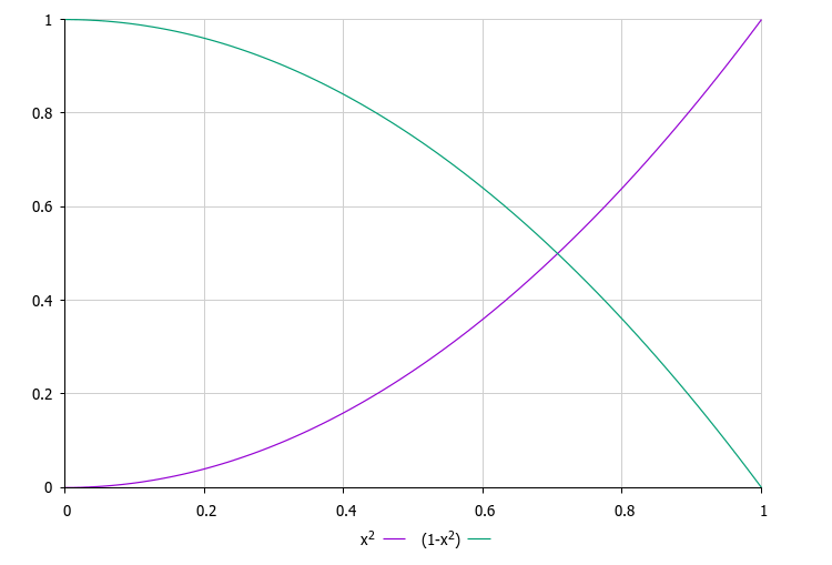
Figure 2. The red line is the probability function of choosing universes depending on their quality, the green line is the degree of change of anchors for the corresponding universes

Algorithm pseudocode:

Initialization:
1. Create a population of N parallel universes
2. For each universe:
   - Randomly initialize the anchor (coordinate) values within acceptable limits
   - Set initial best values equal to current ones

Main loop:
1. Sorting universes by quality (fitness functions)
   - Best universes get lower indices
   - Worst universes get higher indices

2. For each universe i of N:
   For each anchor (coordinate):
   
   a) Select a universe for interaction:
      - Generate a random number rnd from 0 to 1
      - Square rnd to increase the priority of the best universes
      - Select the index of 'pair' proportional to rnd
   
   b) If the current universe does not match the selected one (i ≠ pair):
      
      If the current universe is better than the selected one (i < pair):
         - A slight change in the anchor is proportional to rnd
         - New_value = current + rnd * (selected_value - current)
      
      Otherwise (the current universe is worse than the selected one):
         If (random_number > rnd):
            - Strong change of anchor proportional to (1 - rnd)
            - New_value = current + (1-rnd) * (selected_value - current)
         Otherwise:
            - Complete copying of the anchor value from the best universe
            - New_value = selected_value
   
   c) Otherwise (interaction with oneself):
      - Local search using Gaussian distribution
      - New_value = GaussDistribution(current_best)
   
   d) Correction of the new anchor value within acceptable limits

3. Updating the best values:
   For each universe:
   - If the current solution is better than the personal best, update the personal best
   - If the current solution is better than the global best, update the global best

4. Repeat the main loop until the stopping criterion is met

Now we have everything ready to implement the parallel universe travel machine in code. Let's write the C_AO_TETA class, which will be derived from the C_AO class. Here is a brief description:

• Constructor — initializes the name, description, and link to the algorithm, and sets the population size
• SetParams parameter — sets parameters using values from the "params" array.
• Init, Moving and Revision methods are declared but will be implemented in another piece of code.

class C_AO_TETA : public C_AO
{
  public: //--------------------------------------------------------------------
  ~C_AO_TETA () { }
  C_AO_TETA ()
  {
    ao_name = "TETA";
    ao_desc = "Time Evolution Travel Algorithm";
    ao_link = "https://www.mql5.com/en/articles/16963";

    popSize = 50; // number of parallel universes in the population

    ArrayResize (params, 1);
    params [0].name = "popSize"; params [0].val = popSize;
  }

  void SetParams ()
  {
    popSize = (int)params [0].val;
  }

  bool Init (const double &rangeMinP  [],  // minimum values for anchors
             const double &rangeMaxP  [],  // maximum values for anchors
             const double &rangeStepP [],  // anchor change step
             const int     epochsP = 0);   // number of search epochs

  void Moving ();
  void Revision ();

  private: //-------------------------------------------------------------------
};
//——————————————————————————————————————————————————————————————————————————————

Initialization of the Init method of the C_AO_TETA class performs the initial setup of the algorithm. 

Method parameters:

• rangeMinP — array of minimum values for anchors.
• rangeMaxP — array of maximum values for anchors.
• rangeStepP — array of anchor change steps.
• epochsP — number of search epochs (default 0).

Standard initialization:

• The method calls StandardInit, performs checking and setting ranges for anchors. If initialization fails, return 'false'.

Return value:

• If all checks and settings are successful, the method returns "true", indicating successful initialization of the algorithm.

//——————————————————————————————————————————————————————————————————————————————
// TETA - Time Evolution Travel Algorithm
// An optimization algorithm based on the concept of moving between parallel universes
// through changing the key anchors (events) of life

//——————————————————————————————————————————————————————————————————————————————
bool C_AO_TETA::Init (const double &rangeMinP  [], // minimum values for anchors
                      const double &rangeMaxP  [], // maximum values for anchors
                      const double &rangeStepP [], // anchor change step
                      const int     epochsP = 0)   // number of search epochs
{
  if (!StandardInit (rangeMinP, rangeMaxP, rangeStepP)) return false;

  //----------------------------------------------------------------------------
  return true;
}
//——————————————————————————————————————————————————————————————————————————————

The Moving method of the C_AO_TETA class is responsible for changing anchors in parallel universes to create new ones within the algorithm.

Check the revision status:

• If "revision" is 'false', the method initializes the initial anchor values for all parallel universes using random values from the given range and applying functions to bring them to valid values (based on the step).

Updating anchor values:

• If the revision has already been carried out, an iteration occurs across all parallel universes. For each anchor, a probability is generated and its new value is calculated:
  • If the current universe is more favorable, then the anchor is slightly adjusted in a positive direction to find a better balance.
  • If the current universe is less favorable, a probability test may result in a significant change in the anchor or a complete adoption of the anchor from the more favorable universe.
  • If the universes coincide, a local anchor adjustment occurs using a Gaussian distribution.
• After calculating the new value, the anchor is brought into the acceptable range.

This method is in practice responsible for the adaptation and improvement of solutions (parallel universes), which is a key part of the optimization algorithm. 

//——————————————————————————————————————————————————————————————————————————————
void C_AO_TETA::Moving ()
{
  //----------------------------------------------------------------------------
  if (!revision)
  {
    // Initialize the initial values of anchors in all parallel universes
    for (int i = 0; i < popSize; i++)
    {
      for (int c = 0; c < coords; c++)
      {
        a [i].c [c] = u.RNDfromCI (rangeMin [c], rangeMax [c]);
        a [i].c [c] = u.SeInDiSp  (a [i].c [c], rangeMin [c], rangeMax [c], rangeStep [c]);
      }
    }

    revision = true;
    return;
  }

  //----------------------------------------------------------------------------
  double rnd  = 0.0;
  double val  = 0.0;
  int    pair = 0.0;

  for (int i = 0; i < popSize; i++)
  {
    for (int c = 0; c < coords; c++)
    {
      // Generate a probability that determines the chance of choosing a universe,
      // as well as the anchor change force
      rnd  = u.RNDprobab ();
      rnd *= rnd;

      // Selecting a universe for sharing experience
      pair = (int)u.Scale (rnd, 0.0, 1.0, 0, popSize - 1);

      if (i != pair)
      {
        if (i < pair)
        {
          // If the current universe is more favorable:
          // Slightly change the anchor (proportional to rnd) to find a better balance
          val = a [i].c [c] + (rnd)*(a [pair].cB [c] - a [i].cB [c]);
        }
        else
        {
          if (u.RNDprobab () > rnd)
          {
            // If the current universe is less favorable:
            // Significant change of anchor (proportional to 1.0 - rnd)
            val = a [i].cB [c] + (1.0 - rnd) * (a [pair].cB [c] - a [i].cB [c]);
          }
          else
          {
            // Full acceptance of the anchor configuration from a more successful universe
            val = a [pair].cB [c];
          }
        }
      }
      else
      {
        // Local anchor adjustment via Gaussian distribution
        val = u.GaussDistribution (cB [c], rangeMin [c], rangeMax [c], 1);
      }

      a [i].c [c] = u.SeInDiSp  (val, rangeMin [c], rangeMax [c], rangeStep [c]);
    }
  }
}
//——————————————————————————————————————————————————————————————————————————————

The Revision method of the C_AO_TETA class is responsible for updating the anchor configurations in parallel universes and sorting these universes by their quality. More details:

Updating globally best configuration:

• The method goes through all parallel universes (from 0 to popSize).
• If the value of the f function of the current universe (a[i].f) is greater than the fB global best value, then:
  • fB is updated by the value of (a[i].f).
  • The current universe's anchor configuration is copied to the cB global configuration.

Update the best known configuration for each universe:

• If the value of the f function of the current universe is greater than its best known value (a[i].fB), then:
  • (a[i].fB) is updated by the value of (a[i].f).
  • The current universe's anchor configuration is copied to its best known configuration (a[i].cB).

Sort universes:

• The aT static array is declared to store agents.
• The array size is changed to popSize.
• Universes are sorted by their best known individual properties using the u.Sorting_fB function.

//——————————————————————————————————————————————————————————————————————————————
void C_AO_TETA::Revision ()
{
  for (int i = 0; i < popSize; i++)
  {
    // Update globally best anchor configuration
    if (a [i].f > fB)
    {
      fB = a [i].f;
      ArrayCopy (cB, a [i].c);
    }

    // Update the best known anchor configuration for each universe
    if (a [i].f > a [i].fB)
    {
      a [i].fB = a [i].f;
      ArrayCopy (a [i].cB, a [i].c);
    }
  }

  // Sort universes by their degree of favorability
  static S_AO_Agent aT []; ArrayResize (aT, popSize);
  u.Sorting_fB (a, aT, popSize);
}
//——————————————————————————————————————————————————————————————————————————————

Test results

TETA results:

TETA|Time Evolution Travel Algorithm|50.0|
=============================
5 Hilly's; Func runs: 10000; result: 0.9136198796338938
25 Hilly's; Func runs: 10000; result: 0.8234856192574587
500 Hilly's; Func runs: 10000; result: 0.3199003852163246
=============================
5 Forest's; Func runs: 10000; result: 0.970957820488216
25 Forest's; Func runs: 10000; result: 0.8953189778250419
500 Forest's; Func runs: 10000; result: 0.29324457646900925
=============================
5 Megacity's; Func runs: 10000; result: 0.7346153846153844
25 Megacity's; Func runs: 10000; result: 0.6856923076923078
500 Megacity's; Func runs: 10000; result: 0.16020769230769372
=============================
All score: 5.79704 (64.41%)

Final result: 5.79704 (64.41%). Considering the complexity of the test functions, this is an excellent result. The algorithm very quickly detects important areas of the surface with promising optima and immediately begins refining them, which can be seen in each visualization of the algorithm operation.

TETA on the Hilly test function

  TETA on the Forest test function

TETA on the Megacity test function

Notably, the algorithm achieves the best result among all optimization algorithms, overtaking the leader of the group of population algorithm, on the GoldsteinPrice function included in the set of examples of test functions the optimization algorithms can be tested on.

TETA on GoldsteinPrice test function (available for selection from the list of test functions)

Results on GoldsteinPrice:

5 GoldsteinPrice's; Func runs: 10000; result: 0.9999786723616957
25 GoldsteinPrice's; Func runs: 10000; result: 0.9999750431600845
500 GoldsteinPrice's; Func runs: 10000; result: 0.9992343490683104

Upon completion of the test, the TETA algorithm was among the top ten best optimization algorithms and took a respectable 6th place.

#	AO	Description	Hilly			Hilly final	Forest			Forest final	Megacity (discrete)			Megacity final	Final result	% of MAX
			10 p (5 F)	50 p (25 F)	1000 p (500 F)		10 p (5 F)	50 p (25 F)	1000 p (500 F)		10 p (5 F)	50 p (25 F)	1000 p (500 F)
1	ANS	across neighbourhood search	0.94948	0.84776	0.43857	2.23581	1.00000	0.92334	0.39988	2.32323	0.70923	0.63477	0.23091	1.57491	6.134	68.15
2	CLA	code lock algorithm (joo)	0.95345	0.87107	0.37590	2.20042	0.98942	0.91709	0.31642	2.22294	0.79692	0.69385	0.19303	1.68380	6.107	67.86
3	AMOm	animal migration ptimization M	0.90358	0.84317	0.46284	2.20959	0.99001	0.92436	0.46598	2.38034	0.56769	0.59132	0.23773	1.39675	5.987	66.52
4	(P+O)ES	(P+O) evolution strategies	0.92256	0.88101	0.40021	2.20379	0.97750	0.87490	0.31945	2.17185	0.67385	0.62985	0.18634	1.49003	5.866	65.17
5	CTA	comet tail algorithm (joo)	0.95346	0.86319	0.27770	2.09435	0.99794	0.85740	0.33949	2.19484	0.88769	0.56431	0.10512	1.55712	5.846	64.96
6	TETA	time evolution travel algorithm (joo)	0.91362	0.82349	0.31990	2.05701	0.97096	0.89532	0.29324	2.15952	0.73462	0.68569	0.16021	1.58052	5.797	64.41
7	SDSm	stochastic diffusion search M	0.93066	0.85445	0.39476	2.17988	0.99983	0.89244	0.19619	2.08846	0.72333	0.61100	0.10670	1.44103	5.709	63.44
8	AAm	archery algorithm M	0.91744	0.70876	0.42160	2.04780	0.92527	0.75802	0.35328	2.03657	0.67385	0.55200	0.23738	1.46323	5.548	61.64
9	ESG	evolution of social groups (joo)	0.99906	0.79654	0.35056	2.14616	1.00000	0.82863	0.13102	1.95965	0.82333	0.55300	0.04725	1.42358	5.529	61.44
10	SIA	simulated isotropic annealing (joo)	0.95784	0.84264	0.41465	2.21513	0.98239	0.79586	0.20507	1.98332	0.68667	0.49300	0.09053	1.27020	5.469	60.76
11	ACS	artificial cooperative search	0.75547	0.74744	0.30407	1.80698	1.00000	0.88861	0.22413	2.11274	0.69077	0.48185	0.13322	1.30583	5.226	58.06
12	BHAm	black hole algorithm M	0.75236	0.76675	0.34583	1.86493	0.93593	0.80152	0.27177	2.00923	0.65077	0.51646	0.15472	1.32195	5.196	57.73
13	ASO	anarchy society optimization	0.84872	0.74646	0.31465	1.90983	0.96148	0.79150	0.23803	1.99101	0.57077	0.54062	0.16614	1.27752	5.178	57.54
14	AOSm	atomic orbital search M	0.80232	0.70449	0.31021	1.81702	0.85660	0.69451	0.21996	1.77107	0.74615	0.52862	0.14358	1.41835	5.006	55.63
15	TSEA	turtle shell evolution algorithm (joo)	0.96798	0.64480	0.29672	1.90949	0.99449	0.61981	0.22708	1.84139	0.69077	0.42646	0.13598	1.25322	5.004	55.60
16	DE	differential evolution	0.95044	0.61674	0.30308	1.87026	0.95317	0.78896	0.16652	1.90865	0.78667	0.36033	0.02953	1.17653	4.955	55.06
17	CRO	chemical reaction optimization	0.94629	0.66112	0.29853	1.90593	0.87906	0.58422	0.21146	1.67473	0.75846	0.42646	0.12686	1.31178	4.892	54.36
18	BSA	bird swarm algorithm	0.89306	0.64900	0.26250	1.80455	0.92420	0.71121	0.24939	1.88479	0.69385	0.32615	0.10012	1.12012	4.809	53.44
19	HS	harmony search	0.86509	0.68782	0.32527	1.87818	0.99999	0.68002	0.09590	1.77592	0.62000	0.42267	0.05458	1.09725	4.751	52.79
20	SSG	saplings sowing and growing	0.77839	0.64925	0.39543	1.82308	0.85973	0.62467	0.17429	1.65869	0.64667	0.44133	0.10598	1.19398	4.676	51.95
21	BCOm	bacterial chemotaxis optimization M	0.75953	0.62268	0.31483	1.69704	0.89378	0.61339	0.22542	1.73259	0.65385	0.42092	0.14435	1.21912	4.649	51.65
22	ABO	african buffalo optimization	0.83337	0.62247	0.29964	1.75548	0.92170	0.58618	0.19723	1.70511	0.61000	0.43154	0.13225	1.17378	4.634	51.49
23	(PO)ES	(PO) evolution strategies	0.79025	0.62647	0.42935	1.84606	0.87616	0.60943	0.19591	1.68151	0.59000	0.37933	0.11322	1.08255	4.610	51.22
24	TSm	tabu search M	0.87795	0.61431	0.29104	1.78330	0.92885	0.51844	0.19054	1.63783	0.61077	0.38215	0.12157	1.11449	4.536	50.40
25	BSO	brain storm optimization	0.93736	0.57616	0.29688	1.81041	0.93131	0.55866	0.23537	1.72534	0.55231	0.29077	0.11914	0.96222	4.498	49.98
26	WOAm	wale optimization algorithm M	0.84521	0.56298	0.26263	1.67081	0.93100	0.52278	0.16365	1.61743	0.66308	0.41138	0.11357	1.18803	4.476	49.74
27	AEFA	artificial electric field algorithm	0.87700	0.61753	0.25235	1.74688	0.92729	0.72698	0.18064	1.83490	0.66615	0.11631	0.09508	0.87754	4.459	49.55
28	AEO	artificial ecosystem-based optimization algorithm	0.91380	0.46713	0.26470	1.64563	0.90223	0.43705	0.21400	1.55327	0.66154	0.30800	0.28563	1.25517	4.454	49.49
29	ACOm	ant colony optimization M	0.88190	0.66127	0.30377	1.84693	0.85873	0.58680	0.15051	1.59604	0.59667	0.37333	0.02472	0.99472	4.438	49.31
30	BFO-GA	bacterial foraging optimization - ga	0.89150	0.55111	0.31529	1.75790	0.96982	0.39612	0.06305	1.42899	0.72667	0.27500	0.03525	1.03692	4.224	46.93
31	SOA	simple optimization algorithm	0.91520	0.46976	0.27089	1.65585	0.89675	0.37401	0.16984	1.44060	0.69538	0.28031	0.10852	1.08422	4.181	46.45
32	ABHA	artificial bee hive algorithm	0.84131	0.54227	0.26304	1.64663	0.87858	0.47779	0.17181	1.52818	0.50923	0.33877	0.10397	0.95197	4.127	45.85
33	ACMO	atmospheric cloud model optimization	0.90321	0.48546	0.30403	1.69270	0.80268	0.37857	0.19178	1.37303	0.62308	0.24400	0.10795	0.97503	4.041	44.90
34	ADAMm	adaptive moment estimation M	0.88635	0.44766	0.26613	1.60014	0.84497	0.38493	0.16889	1.39880	0.66154	0.27046	0.10594	1.03794	4.037	44.85
35	ATAm	artificial tribe algorithm M	0.71771	0.55304	0.25235	1.52310	0.82491	0.55904	0.20473	1.58867	0.44000	0.18615	0.09411	0.72026	3.832	42.58
36	ASHA	artificial showering algorithm	0.89686	0.40433	0.25617	1.55737	0.80360	0.35526	0.19160	1.35046	0.47692	0.18123	0.09774	0.75589	3.664	40.71
37	ASBO	adaptive social behavior optimization	0.76331	0.49253	0.32619	1.58202	0.79546	0.40035	0.26097	1.45677	0.26462	0.17169	0.18200	0.61831	3.657	40.63
38	MEC	mind evolutionary computation	0.69533	0.53376	0.32661	1.55569	0.72464	0.33036	0.07198	1.12698	0.52500	0.22000	0.04198	0.78698	3.470	38.55
39	IWO	invasive weed optimization	0.72679	0.52256	0.33123	1.58058	0.70756	0.33955	0.07484	1.12196	0.42333	0.23067	0.04617	0.70017	3.403	37.81
40	Micro-AIS	micro artificial immune system	0.79547	0.51922	0.30861	1.62330	0.72956	0.36879	0.09398	1.19233	0.37667	0.15867	0.02802	0.56335	3.379	37.54
41	COAm	cuckoo optimization algorithm M	0.75820	0.48652	0.31369	1.55841	0.74054	0.28051	0.05599	1.07704	0.50500	0.17467	0.03380	0.71347	3.349	37.21
42	SDOm	spiral dynamics optimization M	0.74601	0.44623	0.29687	1.48912	0.70204	0.34678	0.10944	1.15826	0.42833	0.16767	0.03663	0.63263	3.280	36.44
43	NMm	Nelder-Mead method M	0.73807	0.50598	0.31342	1.55747	0.63674	0.28302	0.08221	1.00197	0.44667	0.18667	0.04028	0.67362	3.233	35.92
44	BBBC	big bang-big crunch algorithm	0.60531	0.45250	0.31255	1.37036	0.52323	0.35426	0.20417	1.08166	0.39769	0.19431	0.11286	0.70486	3.157	35.08
45	CPA	cyclic parthenogenesis algorithm	0.71664	0.40014	0.25502	1.37180	0.62178	0.33651	0.19264	1.15093	0.34308	0.16769	0.09455	0.60532	3.128	34.76
	RW	random walk	0.48754	0.32159	0.25781	1.06694	0.37554	0.21944	0.15877	0.75375	0.27969	0.14917	0.09847	0.52734	2.348	26.09

Summary

While working on the TETA algorithm, I was constantly striving to create something simple and efficient. The metaphor of parallel universes and time travel initially seemed like a simple, neat idea, but during development it organically evolved into an effective optimization mechanism.

The key feature of the algorithm was the idea that it is impossible to achieve perfection in everything at once — you need to find a balance. In life, we constantly balance between family, career, and personal achievements, and it is this concept that I laid at the foundation of the algorithm through the anchor system. Each anchor represents an important aspect that needs to be optimized, but not at the expense of others.

The most interesting technical solution was the connection between the probability of choosing a universe and the strength of its influence on other universes. This created a natural mechanism where the best solutions have a higher chance of being selected, and their influence depends on their quality. This approach provides a balance between exploring new possibilities and using good solutions that have already been found.

Testing the algorithm yielded unexpectedly excellent results. This makes the algorithm particularly valuable for practical problems with limited computational resources. Moreover, the algorithm shows consistently excellent results on different types of functions, demonstrating its versatility. What is especially pleasing is the compactness of the implementation. Only about 50 lines of key code, no customizable parameters, and yet so effective. This is a truly successful solution, where simplicity of implementation is combined with high performance.

Ultimately, TETA exceeded my initial expectations. The time travel metaphor has given birth to a practical and effective optimization tool that can be applied in a wide range of fields. This shows that sometimes simple solutions based on clear natural analogies can be very effective. The algorithm was created literally in one breath — from concept to implementation — and I am very pleased with the work done on the algorithm, which can become a good assistant for researchers and practitioners in quickly finding optimal solutions. 

Figure 3. Color gradation of algorithms according to the corresponding tests

Figure 4. Histogram of algorithm testing results (scale from 0 to 100, the higher the better, where 100 is the maximum possible theoretical result, in the archive there is a script for calculating the rating table)

TETA pros and cons:

Pros:

1. The only external parameter is the population size.
   
2. Simple implementation.
3. Very fast EA.
4. Balanced metrics for both small and large dimensional problems.
   

Disadvantages:

1. Scatter of results on low-dimensional discrete problems.
   

The article is accompanied by an archive with the current versions of the algorithm codes. The author of the article is not responsible for the absolute accuracy in the description of canonical algorithms. Changes have been made to many of them to improve search capabilities. The conclusions and judgments presented in the articles are based on the results of the experiments.

• github: https://github.com/JQSakaJoo/Population-optimization-algorithms-MQL5

Programs used in the article

#	Name	Type	Description
1	#C_AO.mqh	Include	Parent class of population optimization algorithms
2	#C_AO_enum.mqh	Include	Enumeration of population optimization algorithms
3	TestFunctions.mqh	Include	Library of test functions
4	TestStandFunctions.mqh	Include	Test stand function library
5	Utilities.mqh	Include	Library of auxiliary functions
6	CalculationTestResults.mqh	Include	Script for calculating results in the comparison table
7	Testing AOs.mq5	Script	The unified test stand for all population optimization algorithms
8	Simple use of population optimization algorithms.mq5	Script	A simple example of using population optimization algorithms without visualization
9	Test_AO_TETA.mq5	Script	TETA test stand