Artificial Showering Algorithm (ASHA)

Contents

1. Introduction
2. Implementation of the algorithm
3. Test results

Introduction

As data volumes in today's world grow rapidly and tasks become increasingly complex and energy-intensive, the need for effective optimization methods is becoming more urgent than ever. Metaheuristic algorithms with high convergence and processing speed open up new horizons for solving a variety of problems in various fields, from financial markets to scientific research.

The speed of data processing and the quality of the resulting solutions play a key role in the successful implementation of projects. In conditions of strict time constraints, where every moment can be critical, metaheuristic algorithms allow achieving results that previously seemed unattainable. Not only do they provide fast processing of large amounts of information, but they also help to find better solutions compared to traditional numerical methods.

Saving resources is another important aspect to consider when optimizing. In conditions of limited computing power, such algorithms require less time and memory, which is especially valuable in cloud computing. The adaptability of algorithms to changing conditions and the ability to quickly respond to new data make them almost ideal for dynamic systems. This allows us to maintain the relevance of solutions and improve the efficiency of solving problems in real conditions.

Comparing different algorithms by their characteristics, such as convergence rate, solution quality, and resistance to getting stuck in local extremes, makes it possible to select the highest quality ones, which in turn promotes innovation and the development of completely new methods, often inspired by nature, and is an important step in the field of optimization.

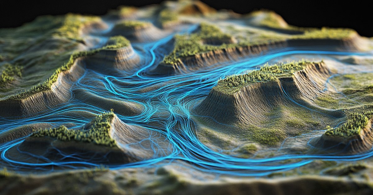
The Artificial Showering Algorithm (ASHA) is a new metaheuristic method developed for solving general optimization problems. The algorithm is based on modeling the flow and accumulation of water distributed by human-controlled equipment on an ideal field. ASHA simulates water distribution (showering) over a field, where water represents resource units and the field is the search space. The algorithm uses the principles of flow and accumulation to find optimal solutions to problems without constraints. The Artificial Showering Algorithm (ASHA) was developed by a group of authors: Ali J., M. Saeed, N.A. Chaudhry, M. Luqman and M. F. Tabassum and published in 2015.

Implementation of the algorithm

The method is based on the following:

1. Ideal field. The search space is an ideal field where water flows without resistance and infiltration occurs only at the lowest point.
2. No external factors. There is no evaporation, no rain, no flow of water.
3. Availability of sprayers. Each part of the search space is within reach of sprayers located above the field.
4. Constant amount of water. There is excess water, and its quantity in the closed system remains constant throughout all iterations.
5. Water movement. Each unit of water has a probabilistic tendency to move downslope.

ASHA (Artificial Showering Algorithm) description step by step.

Algorithm parameters:

• f - objective function to be minimized
• R*n - n-dimensional search space
• K - current position in the iteration counter
• m - number of water units (search agents)
• F - water flow rate
• δ - resistance level (infiltration threshold)
• ρ₀ - initial probability
• β - probability change rate
• M - maximum number of iterations

 Algorithm steps:

1. Initialization:

    Set the initial value ρ = ρ₀
    Create m units of water and place them randomly in the R*n search space

2. Landscape assessment: For each unit of water, we calculate the value of the f objective function at its current position

3. Main loop (repeat M times): for each unit of water i (1 ≤ i ≤ m):

   a) Select a random number r_i ∈ (0, 1)
   b) If r_i < ρ:
       Select a random x_lower position below the current one
       Generate a random vector s ∈ (0, 1)*n
       Calculate a new position:
          x_new = x_old + F × (s ∘ (x_lower  x_old))
          where ∘ denotes element-wise multiplication
       If x_new is at a lower level than x_old:
          Accept a new position
       Otherwise:
          Generate a random number r ∈ (0, 1)
          Find the lowest position x_lowest among all water units
          Calculate the new position:
             x_new = x_old + F × r × (x_lowest  x_old)
   c) Check infiltration:
      If a unit of water has overcome the resistance level of δ:
       Create a new unit of water at a random position
   d) Comparison with the lowest position:
       Find the water unit with the lowest value of the objective function
       If the current unit of water has a lower value, swap them
   e) Update probability ρ = max((M - K) / (β × M), ρ₀)

4. Completion:

    Find the water unit with the smallest value of the objective function
    We return its position as the best solution found

Explanations of the algorithm:

1. The algorithm simulates the process of field showering, where each unit of water represents a search agent.
2. The search space is considered as a landscape, where lower values of the objective function correspond to lower points of the terrain.
3. Water units tend to "flow" to the lower points of the landscape, which corresponds to the search for the minimum of the objective function.
4. The parameter ρ controls the balance between exploration of space (large ρ values) and exploitation of found solutions (small ρ values).
5. The infiltration mechanism avoids getting stuck in local minima by creating new water units in random positions.
6. Comparison and exchange with the lowest position ensures that the best solution found is preserved.
7. Dynamically updating ρ allows the algorithm to gradually move from exploration to exploitation as the number of iterations increases.

The algorithm uses a water flow analogy for optimization, where water (search agents) seeks to find the lowest points in the landscape (minima of the objective function).

According to the authors, the main advantages of this algorithm are:

1. The ability to explore a large solution space thanks to the random movement of water.
2. Ability to avoid local minima using the infiltration mechanism.
3. Adaptive behavior due to dynamic change of ρ probability.

Let's consider in detail all the equations used by the algorithm.

1. Equation for updating position in case of probability fulfillment "ρ": x_new = x_old + F × (s ∘ (x_lower - x_old)), where:

• x_new - new position of the water unit
• x_old - current position of the water unit
• F - water flow rate (algorithm parameter)
• s - random vector in the range (0, 1)
• x_lower - randomly selected position below the current one
  
• ∘ - element-wise multiplication operator

The equation simulates the movement of water down a slope. The random vector s adds an element of randomness to the movement, while F controls the step size.

2. Alternative formula, in case of failure of ρ probability, position update: x_new = x_old + F × r × (x_lowest - x_old), where:

• r - random number in the range (0, 1)
• x_lowest - position with the lowest value of the objective function

The equation is used when the basic formula does not lead to improvement. It directs a water unit towards the global minimum.

As can be seen from these equations, water always tends to move towards positions that are lower than its current position. If the algorithm is implemented only up to this step, it will inevitably get stuck in local extremes.

3. Probability update equation, ρ = max ((M - K) / (β × M), ρ₀), where:

• ρ - current probability of water movement
• M - maximum number of iterations
• K - current iteration number
• β - probability change rate
• ρ₀ - initial probability

This equation gradually reduces the probability of water moving towards randomly selected lower positions and increases the probability of moving towards the global minimum. This allows the algorithm to move from exploring the space to refining the solutions found.

4. Infiltration condition, if f (x_current) < δ, a new water unit is created, where: 

• f (x_current) - value of the objective function at the current position
• δ - resistance level (infiltration threshold)

This condition allows new water units to be created at random positions when the current water unit finds a low enough point. This is intended to avoid getting stuck in local minima.

5. Comparing positions if f (x_i) < f (x_lowest), swap x_i and x_lowest, where:

• f (x_i) - value of the objective function for i th water unit
• f (x_lowest) - smallest found value of the objective function

The equations above form the basis of the ASHA algorithm.

1. The position update equation simulates the movement of water down a slope. A random element (s or r) adds variety to the search by allowing exploration of different areas of the solution space.
2. An alternative position update equation is used with increasing probability with each new iteration to ensure that the degree of refinement of the global solution increases over all iterations.
3. ρ probability update equation provides a balance between exploration and exploitation. At the beginning of the algorithm, the probability of moving towards randomly selected lower positions in the landscape is high, which encourages broad exploration of the space. As iterations progress, the probability decreases, leading to more thorough exploration of promising areas.
4. The infiltration condition allows the algorithm to "restart" the search from new random positions when a good enough solution is found. This helps to avoid getting stuck in local minima.
5. Comparing positions ensures that the algorithm always "remembers" the best solution found and uses it to guide further search.

So the idea is that the algorithm first tries to find a better position by moving towards a random bottom point. If this fails, it tries to move towards the globally best position found. This provides a balance between local search and global exploration of the solution space.

The principle of infiltration in the ASHA algorithm may not be obvious at first glance. Let's take a closer look at it together:

1. We have the δ (delta) parameter, which is called the resistance level or infiltration threshold.
2. At each iteration, for each unit of water, we check whether it has become "too good", that is, whether it has fallen below the level of δ.
3. If the value of the objective function for a given unit of water becomes less than δ, then the water is considered to have "leaked" or "infiltrated" into the ground.
4. In this case, we "create" a new unit of water by placing it at a random position in the search space.

Formally, this can be written as follows: if f (x_i) < δ, x_i = random_position (), where f (x_i) is a value of the objective function for i th field unit, x_i — position of the i th water unit.

The idea behind this mechanism is to avoid getting all water units stuck in a single local minimum; to try to continue exploring the search space even after finding a good solution; and to potentially find even better solutions in unexplored areas.

It is important to choose the right δ value. If δ is too small, infiltration may not occur at all; if δ is too large, the algorithm may constantly "restart" without having time to find the optimal solution. In addition, determining the appropriate value of δ may be a non-trivial task, especially when we do not know the range of values of the objective function in advance and cannot set this parameter as an external one. Therefore, I introduced a counter of attempts to "leak" for each drop, and in the external parameter it is necessary to set its maximum value. With each new attempt, the probability of "leakage" increases according to a quadratic law, that is, with acceleration. This way, no drop will remain in one place for too long, which will help avoid getting stuck in local extremes.

Figure 1. Examples of changes in the probability of infiltration depending on the number of attempts

When it comes to using the coordinates of the lowest point, the following approach is usually used:

1. The unit of water with the smallest value of the objective function is found (let's call it x_lowest).
2. When updating the position, all coordinates of this lowest point are used: x_new = x_old + F × r × (x_lowest - x_old). Here, x_new, x_old and x_lowest are vectors containing all coordinates.
3. This vector equation applies to all coordinates simultaneously. That is, the new position is "attracted" to the lowest point in all dimensions of the search space.

This approach allows us to direct the search to the most promising area of the solution space, taking into account all dimensions simultaneously.

For this algorithm (and, perhaps, if necessary, for subsequent ones), it is necessary to expand the standard structure to store additional information about the optimization agent. The newly entered fields are highlighted in green.

Let's recall what the S_AO_Agent standard structure of the optimization agent, which the user program accesses, looks like. With additions, it looks like this:

1. Structure fields:

• c [] - array of current coordinates of the agent in the search space.
• cP [] - array of previous agent coordinates. 
• cB [] - array of the best coordinates found by the agent over all time.
• f - fitness function value for the current agent coordinates to assess how well the agent copes with the task.
• fP - value of the fitness function for the previous coordinates to track changes in the agent's performance.
• fB - value of the fitness function for the best coordinates preserving the best result achieved by the agent.
• cnt - counter to track the number of iterations.

2. Init () - initialization method takes the number of coordinates required for the agent and performs the following actions:

• changes the c array size up to coords, allocating memory to store the current coordinates.
• similarly changes the size of the cP array to store previous coordinates and the cB array size to store the best coordinates.
• initializes the current value of the fitness function to the minimum possible value, allowing the agent to update it on the first evaluation.
• initializes the previous and best value of the fitness function in a similar way.
• initializes the counter value to zero.

So, the S_AO_Agent structure allows storing information about the current state of the agent, its performance and change history. The changes made to the structure will not affect the optimization algorithms already written on its basis, but will simplify the construction of new algorithms in the future.

//——————————————————————————————————————————————————————————————————————————————
struct S_AO_Agent
{
    double c  []; //coordinates
    double cP []; //previous coordinates
    double cB []; //best coordinates

    double f;     //fitness
    double fP;    //previous fitness
    double fB;    //best fitness

    int    cnt;   //counter

    void Init (int coords)
    {
      ArrayResize (c,  coords);
      ArrayResize (cP, coords);
      ArrayResize (cB, coords);

      f  = -DBL_MAX;
      fP = -DBL_MAX;
      fB = -DBL_MAX;

      cnt = 0;
    }
};
//——————————————————————————————————————————————————————————————————————————————

The C_AO_ASHA class is inherited from the C_AO base class and is an implementation of the ASHA optimization algorithm. Let's analyze its structure and functionality:

• F, δ, β and ρ0 - specific parameters described earlier determine its behavior.
• params - array of structures stores the algorithm parameters. Each array element contains the name of the parameter and its value.

The SetParams () method is used to set the values of algorithm parameters from the params array.

The Init () method initializes the algorithm by taking as input the minimum and maximum search bounds, the search step, and the number of epochs. 

The Moving () and Revision () methods are responsible for moving agents in the search space, for reviewing and updating the state of agents and their positions based on optimization criteria.

Private fields:

• S_AO_Agent aT [] - array for temporary population used for sorting the population.
• epochs - total number of epochs used in the optimization.
• epochNow - current epoch the algorithm is located in.

The C_AO_ASHA class includes the parameters, methods and structures necessary to control the optimization process and interaction of agents.

//——————————————————————————————————————————————————————————————————————————————
class C_AO_ASHA : public C_AO
{
  public: //--------------------------------------------------------------------
  ~C_AO_ASHA () { }
  C_AO_ASHA ()
  {
    ao_name = "ASHA";
    ao_desc = "Artificial Showering Algorithm";
    ao_link = "https://www.mql5.com/en/articles/15980";

    popSize       = 100;  //population size

    F             = 0.3;  //water flow velocity
    δ             = 2;    //resistance level(infiltration threshold)
    β             = 0.8;  //parameter that controls the rate of change in probability
    ρ0            = 0.1;  //initial probability

    ArrayResize (params, 5);

    params [0].name = "popSize"; params [0].val = popSize;
    params [1].name = "F";       params [1].val = F;
    params [2].name = "δ";       params [2].val = δ;
    params [3].name = "β";       params [3].val = β;
    params [4].name = "ρ0";      params [4].val = ρ0;

  }

  void SetParams ()
  {
    popSize = (int)params [0].val;
    F       = params      [1].val;
    δ       = (int)params [2].val;
    β       = params      [3].val;
    ρ0      = params      [4].val;
  }

  bool Init (const double &rangeMinP  [], //minimum search range
             const double &rangeMaxP  [], //maximum search range
             const double &rangeStepP [], //step search
             const int     epochsP = 0);  //number of epochs

  void Moving   ();
  void Revision ();

  //----------------------------------------------------------------------------
  double F;  //water flow velocity
  int    δ;  //resistance level(infiltration threshold)
  double β;  //parameter that controls the rate of change in probability
  double ρ0; //initial probability

  private: //-------------------------------------------------------------------
  S_AO_Agent aT [];
  int  epochs;
  int  epochNow;
};
//——————————————————————————————————————————————————————————————————————————————

The Init method is responsible for initializing the optimization algorithm. Method logic:

1. Standard initialization check: the method calls StandardInit, which performs basic checks and initialization of parameters. 

2. Installation of counters:

• epochs is set equal to the passed epochsP value (the total number of iterations the algorithm should perform).
• epochNow is initialized to zero, the algorithm is just starting to execute and has not yet performed a single epoch.

3. Reserving memory for a temporary population of agents.

4. If all initialization steps are successful, the method returns true, indicating successful initialization of the algorithm.

The Init is key to preparing the algorithm for work. It checks the validity of the inputs, sets the necessary values to control the optimization process, and allocates memory for agents. A successful initialization allows the algorithm to continue performing further operations such as moving and revising agents.

//——————————————————————————————————————————————————————————————————————————————
bool C_AO_ASHA::Init (const double &rangeMinP  [],
                      const double &rangeMaxP  [],
                      const double &rangeStepP [],
                      const int     epochsP = 0)
{
  if (!StandardInit (rangeMinP, rangeMaxP, rangeStepP)) return false;

  //----------------------------------------------------------------------------
  epochs   = epochsP;
  epochNow = 0;

  ArrayResize (aT, popSize);

  return true;
}
//——————————————————————————————————————————————————————————————————————————————

The Moving method implements the logic of moving agents in the search space within the ASHA algorithm. Let's analyze it step by step:

1. The method increments the current epoch counter, allowing us to track the number of iterations performed.

2. Initial initialization (if no revision is required): for each i agent and c coordinate

• the method generates initial positions for all agents within the given ranges using u.RNDfromCI and applies discretization.
• after that, revision is set to true, and the method completes execution.

3. The main loop of the agent movement, for each i agent, the following actions are performed:

• inf - probability calculated using u.Scale to get a value depending on the cnt agent counter. This value is then raised to the fourth power to increase the impact.
• a random number rnd is generated for decision making.

4. Loop through coordinates, for each c coordinate the following actions are performed:

• the ind index is generated to select another agent with a lower position in the search space, which will be used to update the coordinates.
• if i < 1, then: if rnd < inf, then the coordinates of the current agent are updated using a normal distribution around the best coordinates cB by using u.GaussDistribution.
• if i >= 1, then: if rnd < inf, then the coordinates of the current agent are similarly updated relative to the coordinates of another agent a[ind].cB.
• otherwise: the xOld old value remains. If the generated random number is less than ρ:
• xNew is updated based on the best value of another agent xLower.
• otherwise: xNew is updated based on the xLowest global best value.
• then the new value xNew is assigned to the current agent.

5. Coordinate adjustment: Finally, each new coordinate value is adjusted using u.SeInDiSp, so that it fits within the specified ranges and steps.

The Moving method provides both initialization of agent positions and updating them during optimization based on their current state and interaction with other agents.

//——————————————————————————————————————————————————————————————————————————————
void C_AO_ASHA::Moving ()
{
  epochNow++;

  //----------------------------------------------------------------------------
  if (!revision)
  {
    for (int i = 0; i < popSize; i++)
    {
      for (int c = 0; c < coords; c++)
      {
        a [i].c [c] = u.RNDfromCI (rangeMin [c], rangeMax [c]);
        a [i].c [c] = u.SeInDiSp  (a [i].c [c], rangeMin [c], rangeMax [c], rangeStep [c]);
      }
    }

    revision = true;
    return;
  }

  //----------------------------------------------------------------------------
  double xOld    = 0.0;
  double xNew    = 0.0;
  double xLower  = 0.0;
  double xLowest = 0.0;
  double ρ       = MathMax (β * (epochs - epochNow) / epochs, ρ0);
  double inf     = 0.0;
  int    ind     = 0;
  double rnd     = 0.0;

  for (int i = 0; i < popSize; i++)
  {
    inf = u.Scale (a [i].cnt, 0, δ, 0, 1);
    inf = inf * inf * inf * inf;

    rnd = u.RNDprobab ();

    for (int c = 0; c < coords; c++)
    {
      ind = (int)u.RNDintInRange (0, i - 1);
      
      if (i < 1)
      {
        if (rnd < inf)
        {
          a [i].c [c] = u.GaussDistribution (cB [c], rangeMin [c], rangeMax [c], 8);
        }
      }
      else
      {
        if (rnd < inf)
        {
          a [i].c [c] = u.GaussDistribution (a [ind].cB [c], rangeMin [c], rangeMax [c], 8);
        }
        else
        {
          xOld = a [i].c [c];

          if (u.RNDprobab () < ρ)
          {
            xLower = a [ind].cB [c];

            xNew = xOld + F * (u.RNDprobab () * (xLower - xOld));
          }
          else
          {
            xLowest = cB [c];

            xNew = xOld + F * (u.RNDprobab () * (xLowest - xOld));
          }

          a [i].c [c] = xNew;
        }
      }

      a [i].c [c] = u.SeInDiSp  (a [i].c [c], rangeMin [c], rangeMax [c], rangeStep [c]);
    }
  }
}
//——————————————————————————————————————————————————————————————————————————————

The Revision method is responsible for updating information about the best solutions (agents) in the population, as well as tracking their fitness. The steps are described below:

1. The ind variable is initialized by -1. It will be used to store the index of the agent with the best fitness function value of f.

2. Loop over agents: the method loops through all agents in the popSize population:

• if the value of the f fitness function of the current agent exceeds its current best value of fB, then fB is updated and the agent index is saved in the ind variable.
• if the value of the f fitness function of the current agent exceeds its local best value of fB, then the local best value of fB for the agent is updated as well.
• c coordinates of the agent are copied to cB, these are its best known coordinates.
• the cnt counter is reset to 0. Otherwise, if the fitness function value has not improved, the cnt counter is incremented.

3. Copying the best coordinates: if the agent with the best function value (ind is not equal to -1) has been found, then its coordinates are copied to the global variable of cB.

4. Sorting agents: in the end, the u.Sorting_fB is calles to sort the agents by their local best values of fB.

The Revision method plays a central role in the algorithm, monitoring the performance of agents and updating their best known solutions.

//——————————————————————————————————————————————————————————————————————————————
void C_AO_ASHA::Revision ()
{
  //----------------------------------------------------------------------------
  int ind = -1;

  for (int i = 0; i < popSize; i++)
  {
    if (a [i].f > fB)
    {
      fB = a [i].f;
      ind = i;
    }

    if (a [i].f > a [i].fB)
    {
      a [i].fB = a [i].f;
      ArrayCopy (a [i].cB, a [i].c, 0, 0, WHOLE_ARRAY);
      a [i].cnt = 0;
    }
    else
    {
      a [i].cnt++;
    }
  }

  if (ind != -1) ArrayCopy (cB, a [ind].c, 0, 0, WHOLE_ARRAY);

  //----------------------------------------------------------------------------
  u.Sorting_fB (a, aT, popSize);
}
//——————————————————————————————————————————————————————————————————————————————

Test results

The ASHA algorithm test results showed average performance:

ASHA|Artificial Showering Algorithm|100.0|0.3|2.0|0.8|0.1|
=============================
5 Hilly's; Func runs: 10000; result: 0.8968571984324711
25 Hilly's; Func runs: 10000; result: 0.40433437407600525
500 Hilly's; Func runs: 10000; result: 0.25617375427148387
=============================
5 Forest's; Func runs: 10000; result: 0.8036024134603961
25 Forest's; Func runs: 10000; result: 0.35525531625936474
500 Forest's; Func runs: 10000; result: 0.1916000538491299
=============================
5 Megacity's; Func runs: 10000; result: 0.4769230769230769
25 Megacity's; Func runs: 10000; result: 0.1812307692307692
500 Megacity's; Func runs: 10000; result: 0.09773846153846236
=============================
All score: 3.66372 (40.71%)

While observing the work of ASHA during the tests, it is difficult to identify any characteristic features of this algorithm. Isolated studies of promising areas of the search space are not detected.

ASHA on the Hilly test function

ASHA on the Forest test function

ASHA on the Megacity test function

Based on the results of the tests, the ASHA algorithm took 28 th place in the rating table.

#	AO	Description	Hilly			Hilly final	Forest			Forest final	Megacity (discrete)			Megacity final	Final result	% of MAX
			10 p (5 F)	50 p (25 F)	1000 p (500 F)		10 p (5 F)	50 p (25 F)	1000 p (500 F)		10 p (5 F)	50 p (25 F)	1000 p (500 F)
1	ANS	across neighbourhood search	0.94948	0.84776	0.43857	2.23581	1.00000	0.92334	0.39988	2.32323	0.70923	0.63477	0.23091	1.57491	6.134	68.15
2	CLA	code lock algorithm	0.95345	0.87107	0.37590	2.20042	0.98942	0.91709	0.31642	2.22294	0.79692	0.69385	0.19303	1.68380	6.107	67.86
3	AMOm	animal migration ptimization M	0.90358	0.84317	0.46284	2.20959	0.99001	0.92436	0.46598	2.38034	0.56769	0.59132	0.23773	1.39675	5.987	66.52
4	(P+O)ES	(P+O) evolution strategies	0.92256	0.88101	0.40021	2.20379	0.97750	0.87490	0.31945	2.17185	0.67385	0.62985	0.18634	1.49003	5.866	65.17
5	CTA	comet tail algorithm	0.95346	0.86319	0.27770	2.09435	0.99794	0.85740	0.33949	2.19484	0.88769	0.56431	0.10512	1.55712	5.846	64.96
6	SDSm	stochastic diffusion search M	0.93066	0.85445	0.39476	2.17988	0.99983	0.89244	0.19619	2.08846	0.72333	0.61100	0.10670	1.44103	5.709	63.44
7	AAm	archery algorithm M	0.91744	0.70876	0.42160	2.04780	0.92527	0.75802	0.35328	2.03657	0.67385	0.55200	0.23738	1.46323	5.548	61.64
8	ESG	evolution of social groups	0.99906	0.79654	0.35056	2.14616	1.00000	0.82863	0.13102	1.95965	0.82333	0.55300	0.04725	1.42358	5.529	61.44
9	SIA	simulated isotropic annealing	0.95784	0.84264	0.41465	2.21513	0.98239	0.79586	0.20507	1.98332	0.68667	0.49300	0.09053	1.27020	5.469	60.76
10	ACS	artificial cooperative search	0.75547	0.74744	0.30407	1.80698	1.00000	0.88861	0.22413	2.11274	0.69077	0.48185	0.13322	1.30583	5.226	58.06
11	ASO	anarchy society optimization	0.84872	0.74646	0.31465	1.90983	0.96148	0.79150	0.23803	1.99101	0.57077	0.54062	0.16614	1.27752	5.178	57.54
12	TSEA	turtle shell evolution algorithm	0.96798	0.64480	0.29672	1.90949	0.99449	0.61981	0.22708	1.84139	0.69077	0.42646	0.13598	1.25322	5.004	55.60
13	DE	differential evolution	0.95044	0.61674	0.30308	1.87026	0.95317	0.78896	0.16652	1.90865	0.78667	0.36033	0.02953	1.17653	4.955	55.06
14	CRO	chemical reaction optimization	0.94629	0.66112	0.29853	1.90593	0.87906	0.58422	0.21146	1.67473	0.75846	0.42646	0.12686	1.31178	4.892	54.36
15	BSA	bird swarm algorithm	0.89306	0.64900	0.26250	1.80455	0.92420	0.71121	0.24939	1.88479	0.69385	0.32615	0.10012	1.12012	4.809	53.44
16	HS	harmony search	0.86509	0.68782	0.32527	1.87818	0.99999	0.68002	0.09590	1.77592	0.62000	0.42267	0.05458	1.09725	4.751	52.79
17	SSG	saplings sowing and growing	0.77839	0.64925	0.39543	1.82308	0.85973	0.62467	0.17429	1.65869	0.64667	0.44133	0.10598	1.19398	4.676	51.95
18	BCOm	bacterial chemotaxis optimization M	0.75953	0.62268	0.31483	1.69704	0.89378	0.61339	0.22542	1.73259	0.65385	0.42092	0.14435	1.21912	4.649	51.65
19	(PO)ES	(PO) evolution strategies	0.79025	0.62647	0.42935	1.84606	0.87616	0.60943	0.19591	1.68151	0.59000	0.37933	0.11322	1.08255	4.610	51.22
20	TSm	tabu search M	0.87795	0.61431	0.29104	1.78330	0.92885	0.51844	0.19054	1.63783	0.61077	0.38215	0.12157	1.11449	4.536	50.40
21	BSO	brain storm optimization	0.93736	0.57616	0.29688	1.81041	0.93131	0.55866	0.23537	1.72534	0.55231	0.29077	0.11914	0.96222	4.498	49.98
22	WOAm	wale optimization algorithm M	0.84521	0.56298	0.26263	1.67081	0.93100	0.52278	0.16365	1.61743	0.66308	0.41138	0.11357	1.18803	4.476	49.74
23	AEFA	artificial electric field algorithm	0.87700	0.61753	0.25235	1.74688	0.92729	0.72698	0.18064	1.83490	0.66615	0.11631	0.09508	0.87754	4.459	49.55
24	ACOm	ant colony optimization M	0.88190	0.66127	0.30377	1.84693	0.85873	0.58680	0.15051	1.59604	0.59667	0.37333	0.02472	0.99472	4.438	49.31
25	BFO-GA	bacterial foraging optimization - ga	0.89150	0.55111	0.31529	1.75790	0.96982	0.39612	0.06305	1.42899	0.72667	0.27500	0.03525	1.03692	4.224	46.93
26	ABHA	artificial bee hive algorithm	0.84131	0.54227	0.26304	1.64663	0.87858	0.47779	0.17181	1.52818	0.50923	0.33877	0.10397	0.95197	4.127	45.85
27	ACMO	atmospheric cloud model optimization	0.90321	0.48546	0.30403	1.69270	0.80268	0.37857	0.19178	1.37303	0.62308	0.24400	0.10795	0.97503	4.041	44.90
28	ASHA	artificial showering algorithm	0.89686	0.40433	0.25617	1.55737	0.80360	0.35526	0.19160	1.35046	0.47692	0.18123	0.09774	0.75589	3.664	40.71
29	ASBO	adaptive social behavior optimization	0.76331	0.49253	0.32619	1.58202	0.79546	0.40035	0.26097	1.45677	0.26462	0.17169	0.18200	0.61831	3.657	40.63
30	MEC	mind evolutionary computation	0.69533	0.53376	0.32661	1.55569	0.72464	0.33036	0.07198	1.12698	0.52500	0.22000	0.04198	0.78698	3.470	38.55
31	IWO	invasive weed optimization	0.72679	0.52256	0.33123	1.58058	0.70756	0.33955	0.07484	1.12196	0.42333	0.23067	0.04617	0.70017	3.403	37.81
32	Micro-AIS	micro artificial immune system	0.79547	0.51922	0.30861	1.62330	0.72956	0.36879	0.09398	1.19233	0.37667	0.15867	0.02802	0.56335	3.379	37.54
33	COAm	cuckoo optimization algorithm M	0.75820	0.48652	0.31369	1.55841	0.74054	0.28051	0.05599	1.07704	0.50500	0.17467	0.03380	0.71347	3.349	37.21
34	SDOm	spiral dynamics optimization M	0.74601	0.44623	0.29687	1.48912	0.70204	0.34678	0.10944	1.15826	0.42833	0.16767	0.03663	0.63263	3.280	36.44
35	NMm	Nelder-Mead method M	0.73807	0.50598	0.31342	1.55747	0.63674	0.28302	0.08221	1.00197	0.44667	0.18667	0.04028	0.67362	3.233	35.92
36	FAm	firefly algorithm M	0.58634	0.47228	0.32276	1.38138	0.68467	0.37439	0.10908	1.16814	0.28667	0.16467	0.04722	0.49855	3.048	33.87
37	GSA	gravitational search algorithm	0.64757	0.49197	0.30062	1.44016	0.53962	0.36353	0.09945	1.00260	0.32667	0.12200	0.01917	0.46783	2.911	32.34
38	BFO	bacterial foraging optimization	0.61171	0.43270	0.31318	1.35759	0.54410	0.21511	0.05676	0.81597	0.42167	0.13800	0.03195	0.59162	2.765	30.72
39	ABC	artificial bee colony	0.63377	0.42402	0.30892	1.36671	0.55103	0.21874	0.05623	0.82600	0.34000	0.14200	0.03102	0.51302	2.706	30.06
40	BA	bat algorithm	0.59761	0.45911	0.35242	1.40915	0.40321	0.19313	0.07175	0.66810	0.21000	0.10100	0.03517	0.34617	2.423	26.93
41	AAA	algae adaptive algorithm	0.50007	0.32040	0.25525	1.07572	0.37021	0.22284	0.16785	0.76089	0.27846	0.14800	0.09755	0.52402	2.361	26.23
42	SA	simulated annealing	0.55787	0.42177	0.31549	1.29513	0.34998	0.15259	0.05023	0.55280	0.31167	0.10033	0.02883	0.44083	2.289	25.43
43	IWDm	intelligent water drops M	0.54501	0.37897	0.30124	1.22522	0.46104	0.14704	0.04369	0.65177	0.25833	0.09700	0.02308	0.37842	2.255	25.06
44	PSO	particle swarm optimisation	0.59726	0.36923	0.29928	1.26577	0.37237	0.16324	0.07010	0.60572	0.25667	0.08000	0.02157	0.35823	2.230	24.77
45	Boids	boids algorithm	0.43340	0.30581	0.25425	0.99346	0.35718	0.20160	0.15708	0.71586	0.27846	0.14277	0.09834	0.51957	2.229	24.77

Summary

I liked the idea of the algorithm, but during implementation and testing, I had the feeling that the algorithm was missing something. The algorithm is not among the weakest, but it is far from the best. This creates an opportunity for researchers to continue working with it, especially due to its simplicity, since the idea itself, in my opinion, is very promising. In addition, the authors did not provide a more detailed explanation of the infiltration ratio, which allows it to be interpreted in different ways, limited only by the researcher's imagination.

The main conclusion that can be drawn from this article is that not every simple idea is as effective as a more complex one. The efficiency of an optimization algorithm is a complex matter and involves trade-offs. I hope that this algorithm will become another page in the big book of knowledge about the subtleties and tricks of the art of finding the best solutions.

Figure 2. Color gradation of algorithms according to relevant tests Results greater than or equal to 0.99 are highlighted in white

Figure 3. The histogram of algorithm test results (on a scale from 0 to 100, the more the better,

where 100 is the maximum possible theoretical result, the archive features a script for calculating the rating table)

ASHA pros and cons:

Pros:

1. Fast.
   
2. Simple implementation.
   

Cons:

1. Low convergence accuracy.
   

The article is accompanied by an archive with the current versions of the algorithm codes. The author of the article is not responsible for the absolute accuracy in the description of canonical algorithms. Changes have been made to many of them to improve search capabilities. The conclusions and judgments presented in the articles are based on the results of the experiments.

• github: https://github.com/JQSakaJoo/Population-optimization-algorithms-MQL5