Black Hole Algorithm (BHA)
Contents
Introduction
Black Hole Algorithm (BHA) offers a unique perspective on the optimization problem. Created in 2013 by A. Hatamlou, this algorithm draws inspiration from the most mysterious and powerful objects in the universe: black holes. Just as black holes attract everything around them with their gravitational field, the algorithm seeks to "attract" the best solutions to itself, cutting off the less successful ones.
Imagine a vast space filled with many decisions, each struggling to survive in this harsh environment. At the center of this chaos are black holes - solutions with the highest quality ratings that have the force of gravity. The black hole algorithm makes decisions at each step about which stars will be swallowed by black holes and which will continue on their way in search of more favorable conditions.
With elements of randomness, the BHA algorithm explores uncharted areas, trying to avoid local minima traps. This makes it a powerful tool for solving complex problems, from function optimization to combinatorial problems and even hyperparameter tuning in machine learning. In this article, we will take a detailed look at the Black Hole Algorithm, how it works, and its advantages and disadvantages, opening up a world where the science and art of optimization intertwine.
Implementation of the algorithm
The BHA algorithm uses ideas about how stars interact with a black hole to find optimal solutions in a given search space. The algorithm operation begins with initialization, where an initial population of random "stars" is created, each of which represents a potential solution to the optimization problem. These stars are located in a search space bound by upper and lower limits. During the iterations of the algorithm, at each step the best solution is selected, which is designated as a "black hole". The remaining stars tend to move closer to the black hole using the following equation:
Xi(t+1) = Xi(t) + rand × (XBH - Xi(t))
where:
- Xi(t) — current position of i star
- XBH — black hole position
- rand — random number from 0 to 1
An important element of the algorithm is the event horizon calculated using the equation:
R = fitBH / Σfiti
Stars that cross this horizon are "swallowed" by the black hole and replaced by new random stars. This mechanism maintains population diversity and promotes further exploration of space.
The black hole algorithm has several key characteristics. It has a simple structure and no parameters at all except the population size, making it easy to use. It requires no tuning, which is almost unheard of in other optimization algorithms.
The BHA algorithm is similar to other population-based algorithms, meaning that the first step in the optimization is to create an initial population of random solutions (initial stars) and compute an objective function to estimate the solution values. The best solution in each iteration is selected like a black hole, which then begins to attract other candidate solutions around it. They are called stars. If other candidate solutions approach the best obtained solution, they will be "absorbed" by the best solution.
The figure below shows a demonstration of the BHA algorithm search strategy in action. All stars beyond the black hole's event horizon are moved toward its center, and stars that cross the horizon are absorbed — essentially, the star matter will be teleported to a new region of search space.
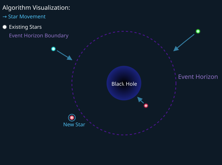
Figure 1. BHA search strategy. The green and blue stars move towards the center of the black hole, and the red star teleports to the "New Star" point.
Let's write a pseudocode for the Black Hole Algorithm (BHA)
N - number of stars (population size)
tmax - maximum number of iterations
// Initialization
1. Create initial positions for N stars:
For i = 1 to N:
Xi = LB + rand × (UB - LB)
2. t = 1
// Main loop
3. While t ≤ tmax:
// Calculate the objective function value for each star
4. For each Xi calculate fiti
// Define a black hole
5. Determine XBH as the star with the best fiti value
fitBH = best fiti value
// Update star positions
6. For each Xi star:
Xi(t+1) = Xi(t) + rand × (XBH - Xi(t))
// Calculate the radius of the event horizon
7. R = fitBH / ∑(i=1 to N) fiti
// Check star absorption
8. For each Xi star:
If the distance between Xi and XBH < R:
Generate a new position for Xi randomly
Xi = LB + rand × (UB - LB)
9. t = t + 1
// Return the best solution found
Return XBH
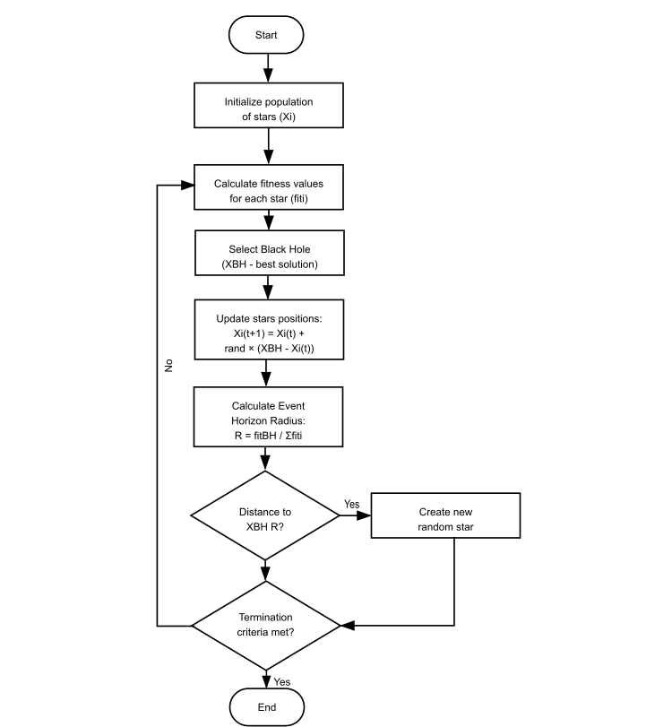
Figure 2. Logical structure of the BHA algorithm operation
Definition of the C_AO_BHA (Black Hole Algorithm) class, which is a descendant of the C_AO base class, class structure:
Constructor and destructor:
- The constructor initializes the basic parameters of the algorithm.
- SetParams () - set the population size from the parameter array
- Init () - initialize the search space with the given boundaries and step
- Moving () - implement the movement of stars towards a black hole
- Revision () - update the best solution found (black hole)
- blackHoleIndex - store the index of the best solution in the population
- rangeMinP [] - minimum values for each coordinate
- rangeMaxP [] - maximum values for each coordinate
- rangeStepP [] - discretization step for each coordinate
- epochsP - number of algorithm iterations
This is a basic framework for implementing the black hole algorithm, where the main logic will be implemented in the Moving() and Revision() methods.
//——————————————————————————————————————————————————————————————————————————————
class C_AO_BHA : public C_AO
{
  public: //--------------------------------------------------------------------
  ~C_AO_BHA () { }
  C_AO_BHA ()
  {
    ao_name = "BHA";
    ao_desc = "Black Hole Algorithm";
    ao_link = "https://www.mql5.com/en/articles/16655";

    popSize = 50;   // Population size

    ArrayResize (params, 1);

    // Initialize parameters
    params [0].name = "popSize"; params [0].val = popSize;
  }

  void SetParams () // Method for setting parameters
  {
    popSize = (int)params [0].val;
  }

  bool Init (const double &rangeMinP  [], // Minimum search range
             const double &rangeMaxP  [], // Maximum search range
             const double &rangeStepP [], // Search step
             const int     epochsP = 0);  // Number of epochs

  void Moving   ();       // Moving method
  void Revision ();       // Revision method

  private: //-------------------------------------------------------------------
  int blackHoleIndex;    // Black hole index (best solution)
};
The Init method is simple and its task is as follows:
- Initialize the algorithm
- Call StandardInit for setting search ranges and step
- Set the initial index of the black hole to 0
- Return 'true' in case of successful initialization, 'false' in case of an error.
//——————————————————————————————————————————————————————————————————————————————
bool C_AO_BHA::Init (const double &rangeMinP  [],
                     const double &rangeMaxP  [],
                     const double &rangeStepP [],
                     const int     epochsP = 0)
{
  if (!StandardInit (rangeMinP, rangeMaxP, rangeStepP)) return false;

  blackHoleIndex = 0; // Initialize black hole index
  return true;
}
//——————————————————————————————————————————————————————————————————————————————
The Moving method consists of several main blocks:
a) Primary initialization (if revision = false):
- Create an initial population of stars with random positions
- Positions are generated in a given range and reduced to a discrete grid
- Set revision flag to true
b) Basic algorithm (if revision = true):
- Calculate the sum of the fitness function values of all stars
- Calculate the radius of the event horizon: R = fitBH / Σfiti
c) Update star positions:
- For each star (except a black hole):
- Calculate the Euclidean distance to a black hole
- If the distance is less than the horizon radius:
- Create a new random star
- Else:
- Update the position using the equation: Xi(t+1) = Xi(t) + rand × (XBH - Xi(t))
- Bring the new position into the acceptable range and discrete grid
All calculations are performed taking into account the limitations of the search space and the discretization step.
//——————————————————————————————————————————————————————————————————————————————
void C_AO_BHA::Moving ()
{
  // Initial random positioning on first run
  if (!revision)
  {
    for (int i = 0; i < popSize; i++)
    {
      for (int c = 0; c < coords; c++)
      {
        // Generate a random position within the allowed range
        a [i].c [c] = u.RNDfromCI (rangeMin [c], rangeMax [c]);
        // Convert to discrete values according to step
        a [i].c [c] = u.SeInDiSp (a [i].c [c], rangeMin [c], rangeMax [c], rangeStep [c]);
      }
    }
    revision = true;
    return;
  }

  // Calculate the sum of fitness values for the radius of the event horizon
  double sumFitness = 0.0;
  for (int i = 0; i < popSize; i++)
  {
    sumFitness += a [i].f;
  }

  // Calculate the radius of the event horizon
  // R = fitBH / Σfiti
  double eventHorizonRadius = a [blackHoleIndex].f / sumFitness;

  // Update star positions
  for (int i = 0; i < popSize; i++)
  {
    // Skip the black hole
    if (i == blackHoleIndex) continue;

    // Calculate the distance to the black hole
    double distance = 0.0;
    for (int c = 0; c < coords; c++)
    {
      double diff = a [blackHoleIndex].c [c] - a [i].c [c];
      distance += diff * diff;
    }
    distance = sqrt (distance);

    // Check for event horizon crossing
    if (distance < eventHorizonRadius)
    {
      // Star is consumed - create a new random star
      for (int c = 0; c < coords; c++)
      {
        a [i].c [c] = u.RNDfromCI (rangeMin [c], rangeMax [c]);
        a [i].c [c] = u.SeInDiSp (a [i].c [c], rangeMin [c], rangeMax [c], rangeStep [c]);
      }
    }
    else
    {
      // Update the star position using the equation:
      // Xi(t+1) = Xi(t) + rand × (XBH - Xi(t))
      for (int c = 0; c < coords; c++)
      {
        double rnd = u.RNDfromCI (0.0, 1.0);
        double newPosition = a [i].c [c] + rnd * (a [blackHoleIndex].c [c] - a [i].c [c]);

        // Check and correct the boundaries
        newPosition = u.SeInDiSp (newPosition, rangeMin [c], rangeMax [c], rangeStep [c]);
        a [i].c [c] = newPosition;
      }
    }
  }
}
//——————————————————————————————————————————————————————————————————————————————
The Revision method performs the following functions:
Find the best solution:
- Iterate through all the stars in the population
- Compare the fitness value of each star (a[i].f) with the current best value (fB)
- When finding the best solution:
- Update the best fitness function value (fB)
- Store the black hole index (blackHoleIndex)
- Copy the coordinates of the best solution to the cB array
The main goal of the method is to track and save the best found solution (black hole) during the optimization.
//——————————————————————————————————————————————————————————————————————————————
void C_AO_BHA::Revision ()
{
  // Find the best solution (black hole)
  for (int i = 0; i < popSize; i++)
  {
    if (a [i].f > fB)
    {
      fB = a [i].f;
      blackHoleIndex = i;
      ArrayCopy (cB, a [i].c, 0, 0, WHOLE_ARRAY);
    }
  }
}
//——————————————————————————————————————————————————————————————————————————————
Testing the BHA algorithm showed the following results:
BHA|Black Hole Algorithm|50.0|
=============================
5 Hilly's; Func runs: 10000; result: 0.6833993073000924
25 Hilly's; Func runs: 10000; result: 0.47275633991339616
500 Hilly's; Func runs: 10000; result: 0.2782882943201518
=============================
5 Forest's; Func runs: 10000; result: 0.6821776337288085
25 Forest's; Func runs: 10000; result: 0.3878950941651221
500 Forest's; Func runs: 10000; result: 0.20702263338385946
=============================
5 Megacity's; Func runs: 10000; result: 0.39461538461538465
25 Megacity's; Func runs: 10000; result: 0.20076923076923076
500 Megacity's; Func runs: 10000; result: 0.1076846153846164
=============================
All score: 3.41461 (37.94%)
The results are below average, according to the table. However, the obvious advantage of this algorithm is that it has no parameters other than the population size, which allows us to consider the results quite satisfactory. During its operation, I immediately noticed that it was stuck in local optima caused by a lack of diversity in the population decisions. In addition, for each star, it is necessary to perform resource-intensive calculations of the Euclidean distance to the black hole. This circumstance prompted reflection on possible ways to correct existing shortcomings.
In the original algorithm, when an iteration occurs, the stars move while the black hole remains in place, even though all objects in space are in motion. I decided to make some changes and implement the black hole moving at distances determined by a Gaussian distribution relative to its center, and also try a power law distribution. This adaptation was aimed at improving the convergence accuracy while maintaining the ability to explore new regions of the solution space. However, despite these changes, the results did not show improvement. This may indicate that the stable position of the black hole (specifically for a given search strategy) is important for the efficiency of the algorithm, ensuring that the stars are focused on the most promising areas. It may be worth considering other approaches or combinations of methods to achieve greater improvements in results.
So the idea came up to move away from calculating Euclidean distances and instead use the event horizon of a black hole as a measure of probabilistic absorption, rather than the actual crossing of the horizon. Instead of applying the motion to the entire star, apply this probability separately to each coordinate.
Then, based on the above considerations, we will write a new version of the Moving method. The changes affected the method of calculating the event horizon, where the average fitness value for the population is now normalized to the distance between the minimum and maximum fitness for the population. Now the event horizon is the probability of absorption at individual coordinates of stars; if absorption does not occur, then we perform the usual movement towards the center of the galactic black monster according to the author's equation.
//——————————————————————————————————————————————————————————————————————————————
void C_AO_BHAm::Moving ()
{
  // Initial random positioning on first run
  if (!revision)
  {
    for (int i = 0; i < popSize; i++)
    {
      for (int c = 0; c < coords; c++)
      {
        // Generate a random position within the allowed range
        a [i].c [c] = u.RNDfromCI (rangeMin [c], rangeMax [c]);
        // Convert to discrete values according to step
        a [i].c [c] = u.SeInDiSp (a [i].c [c], rangeMin [c], rangeMax [c], rangeStep [c]);
      }
    }
    revision = true;
    return;
  }

  //----------------------------------------------------------------------------
  // Calculate the average fitness values for the event horizon radius
  double aveFit = 0.0;
  double maxFit = fB;
  double minFit = a [0].f;

  for (int i = 0; i < popSize; i++)
  {
    aveFit += a [i].f;
    if (a [i].f < minFit) minFit = a [i].f;
  }
  aveFit /= popSize;

  // Calculate the radius of the event horizon
  double eventHorizonRadius = (aveFit - minFit) / (maxFit - minFit);

  // Update star positions
  for (int i = 0; i < popSize; i++)
  {
    // Skip the black hole
    if (i == blackHoleIndex) continue;

    for (int c = 0; c < coords; c++)
    {
      if (u.RNDprobab () < eventHorizonRadius * 0.01)
      {
        a [i].c [c] = u.RNDfromCI (rangeMin [c], rangeMax [c]);
        a [i].c [c] = u.SeInDiSp (a [i].c [c], rangeMin [c], rangeMax [c], rangeStep [c]);
      }
      else
      {
        double rnd = u.RNDfromCI (0.0, 1.0);
        double newPosition = a [i].c [c] + rnd * (a [blackHoleIndex].c [c] - a [i].c [c]);

        // Check and correct the boundaries
        newPosition = u.SeInDiSp (newPosition, rangeMin [c], rangeMax [c], rangeStep [c]);
        a [i].c [c] = newPosition;
      }
    }
  }
}
//——————————————————————————————————————————————————————————————————————————————
Let's analyze the key differences between the two versions of the algorithm, starting with the calculation of the event horizon radius. In the first version (BHA), the radius is defined as the ratio of the best solution to the sum of all solutions, which leads to the fact that for a large population the radius becomes very small and strongly depends on the absolute values of the fitness function. In the second version (BHAm), the radius is normalized in the range [0,1], which allows it to show the relative position of the mean between the minimum and maximum, while maintaining independence from the population size and the absolute values of the fitness function.
Now let's look at the mechanism of star absorption. The first version of the algorithm checks the Euclidean distance to the black hole, and when it is absorbed, the star is completely replaced by a new one in a random location, which leads to more dramatic changes in the population. The second version uses probabilistic absorption for each coordinate separately, which provides smoother changes in the population. Here the ratio of 0.01 reduces the probability of radical changes.
In terms of consequences, the first version exhibits a more aggressive exploitation of the search space, which leads to fast convergence in local regions, but also increases the risk of premature convergence and may miss promising regions due to complete replacement of solutions. The second version, in contrast, offers a more relaxed exploration strategy, providing a better balance between exploration and exploitation, less risk of getting stuck in local optima, and slower but potentially more reliable convergence, as well as a better ability to diversify the population.
In conclusion, the first version is better suited for problems with clearly defined optima, when fast convergence and small dimensions of the search space are required, while the second version is more effective for complex multi-extremal problems, where the reliability of the search for the global optimum is important, as well as for high-dimensional problems that require a more thorough exploration of the search space.
I would like to share my thoughts on visualizing the work of algorithms. Visualization provides a unique opportunity to gain a deeper understanding of the internal processes occurring in algorithms and to reveal their hidden mechanisms. With certain settings, we can observe how chaotic images gradually transform into structured patterns. This process not only demonstrates the technical aspects of the algorithm's operation, but also opens up new ideas and approaches to its optimization.
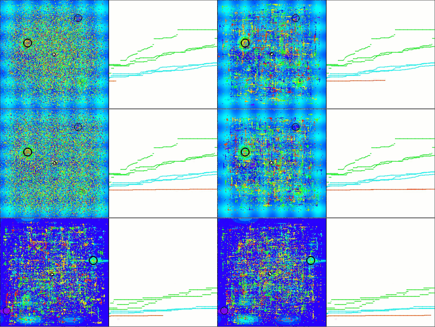
The example of the BHAm algorithm in generating a random component of star movement in the range [0.0;0.1]
It is important to note that visualization allows us not only to evaluate the efficiency of algorithms, but also to identify patterns that may not be obvious with traditional data analysis. This helps to develop a deeper understanding of their work and can inspire new solutions and innovations. Thus, visualization becomes a powerful tool that helps connect science and creativity, opening up new horizons for exploring and understanding complex processes.
Test results
Results of the modified version of the BHAm algorithm:
BHAm|Black Hole Algorithm M|50.0|
=============================
5 Hilly's; Func runs: 10000; result: 0.752359491007831
25 Hilly's; Func runs: 10000; result: 0.7667459889455067
500 Hilly's; Func runs: 10000; result: 0.34582657277589457
=============================
5 Forest's; Func runs: 10000; result: 0.9359337849703726
25 Forest's; Func runs: 10000; result: 0.801524710041611
500 Forest's; Func runs: 10000; result: 0.2717683112397725
=============================
5 Megacity's; Func runs: 10000; result: 0.6507692307692307
25 Megacity's; Func runs: 10000; result: 0.5164615384615385
500 Megacity's; Func runs: 10000; result: 0.154715384615386
=============================
All score: 5.19611 (57.73%)
Based on the test results, the BHAm algorithm shows impressive results, not only in comparison with the original version, but also in the table as a whole. The visualization shows that the new version with the "m" postfix is indeed free from the characteristic shortcomings of the original: the tendency to get stuck is practically eliminated, the accuracy of convergence is significantly increased, and the scatter of results is reduced. At the same time, the "family trait" of the original algorithm is preserved: the formation of peculiar clumps of stars in space and attraction to a certain attractor in the solution space.
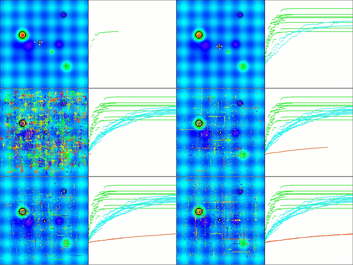
BHAm on the Hilly test function
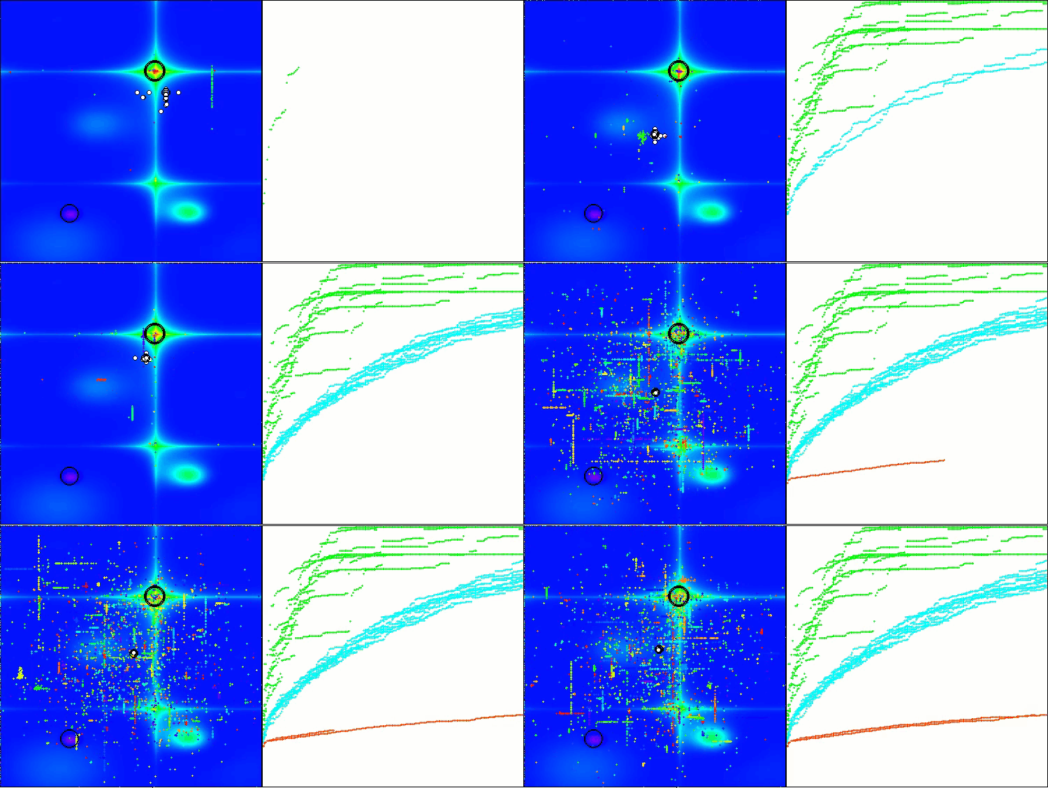
BHAm on the Forest test function
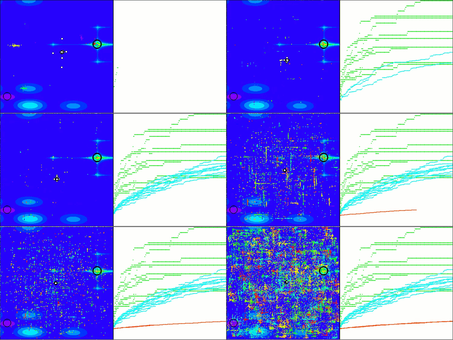
BHAm on the Megacity test function
Based on the test results, the BHAm algorithm took the honorable 11th place, which is a very good result, considering the presence of the most powerful known algorithms as competitors.
| # | AO | Description | Hilly | Hilly final | Forest | Forest final | Megacity (discrete) | Megacity final | Final result | % of MAX | ||||||
| 10 p (5 F) | 50 p (25 F) | 1000 p (500 F) | 10 p (5 F) | 50 p (25 F) | 1000 p (500 F) | 10 p (5 F) | 50 p (25 F) | 1000 p (500 F) | ||||||||
| 1 | ANS | across neighbourhood search | 0.94948 | 0.84776 | 0.43857 | 2.23581 | 1.00000 | 0.92334 | 0.39988 | 2.32323 | 0.70923 | 0.63477 | 0.23091 | 1.57491 | 6.134 | 68.15 |
| 2 | CLA | code lock algorithm (joo) | 0.95345 | 0.87107 | 0.37590 | 2.20042 | 0.98942 | 0.91709 | 0.31642 | 2.22294 | 0.79692 | 0.69385 | 0.19303 | 1.68380 | 6.107 | 67.86 |
| 3 | AMOm | animal migration ptimization M | 0.90358 | 0.84317 | 0.46284 | 2.20959 | 0.99001 | 0.92436 | 0.46598 | 2.38034 | 0.56769 | 0.59132 | 0.23773 | 1.39675 | 5.987 | 66.52 |
| 4 | (P+O)ES | (P+O) evolution strategies | 0.92256 | 0.88101 | 0.40021 | 2.20379 | 0.97750 | 0.87490 | 0.31945 | 2.17185 | 0.67385 | 0.62985 | 0.18634 | 1.49003 | 5.866 | 65.17 |
| 5 | CTA | comet tail algorithm (joo) | 0.95346 | 0.86319 | 0.27770 | 2.09435 | 0.99794 | 0.85740 | 0.33949 | 2.19484 | 0.88769 | 0.56431 | 0.10512 | 1.55712 | 5.846 | 64.96 |
| 6 | SDSm | stochastic diffusion search M | 0.93066 | 0.85445 | 0.39476 | 2.17988 | 0.99983 | 0.89244 | 0.19619 | 2.08846 | 0.72333 | 0.61100 | 0.10670 | 1.44103 | 5.709 | 63.44 |
| 7 | AAm | archery algorithm M | 0.91744 | 0.70876 | 0.42160 | 2.04780 | 0.92527 | 0.75802 | 0.35328 | 2.03657 | 0.67385 | 0.55200 | 0.23738 | 1.46323 | 5.548 | 61.64 |
| 8 | ESG | evolution of social groups (joo) | 0.99906 | 0.79654 | 0.35056 | 2.14616 | 1.00000 | 0.82863 | 0.13102 | 1.95965 | 0.82333 | 0.55300 | 0.04725 | 1.42358 | 5.529 | 61.44 |
| 9 | SIA | simulated isotropic annealing (joo) | 0.95784 | 0.84264 | 0.41465 | 2.21513 | 0.98239 | 0.79586 | 0.20507 | 1.98332 | 0.68667 | 0.49300 | 0.09053 | 1.27020 | 5.469 | 60.76 |
| 10 | ACS | artificial cooperative search | 0.75547 | 0.74744 | 0.30407 | 1.80698 | 1.00000 | 0.88861 | 0.22413 | 2.11274 | 0.69077 | 0.48185 | 0.13322 | 1.30583 | 5.226 | 58.06 |
| 11 | BHAm | black hole algorithm M | 0.75236 | 0.76675 | 0.34583 | 1.86493 | 0.93593 | 0.80152 | 0.27177 | 2.00923 | 0.65077 | 0.51646 | 0.15472 | 1.32195 | 5.196 | 57.73 |
| 12 | ASO | anarchy society optimization | 0.84872 | 0.74646 | 0.31465 | 1.90983 | 0.96148 | 0.79150 | 0.23803 | 1.99101 | 0.57077 | 0.54062 | 0.16614 | 1.27752 | 5.178 | 57.54 |
| 13 | AOSm | atomic orbital search M | 0.80232 | 0.70449 | 0.31021 | 1.81702 | 0.85660 | 0.69451 | 0.21996 | 1.77107 | 0.74615 | 0.52862 | 0.14358 | 1.41835 | 5.006 | 55.63 |
| 14 | TSEA | turtle shell evolution algorithm (joo) | 0.96798 | 0.64480 | 0.29672 | 1.90949 | 0.99449 | 0.61981 | 0.22708 | 1.84139 | 0.69077 | 0.42646 | 0.13598 | 1.25322 | 5.004 | 55.60 |
| 15 | DE | differential evolution | 0.95044 | 0.61674 | 0.30308 | 1.87026 | 0.95317 | 0.78896 | 0.16652 | 1.90865 | 0.78667 | 0.36033 | 0.02953 | 1.17653 | 4.955 | 55.06 |
| 16 | CRO | chemical reaction optimization | 0.94629 | 0.66112 | 0.29853 | 1.90593 | 0.87906 | 0.58422 | 0.21146 | 1.67473 | 0.75846 | 0.42646 | 0.12686 | 1.31178 | 4.892 | 54.36 |
| 17 | BSA | bird swarm algorithm | 0.89306 | 0.64900 | 0.26250 | 1.80455 | 0.92420 | 0.71121 | 0.24939 | 1.88479 | 0.69385 | 0.32615 | 0.10012 | 1.12012 | 4.809 | 53.44 |
| 18 | HS | harmony search | 0.86509 | 0.68782 | 0.32527 | 1.87818 | 0.99999 | 0.68002 | 0.09590 | 1.77592 | 0.62000 | 0.42267 | 0.05458 | 1.09725 | 4.751 | 52.79 |
| 19 | SSG | saplings sowing and growing | 0.77839 | 0.64925 | 0.39543 | 1.82308 | 0.85973 | 0.62467 | 0.17429 | 1.65869 | 0.64667 | 0.44133 | 0.10598 | 1.19398 | 4.676 | 51.95 |
| 20 | BCOm | bacterial chemotaxis optimization M | 0.75953 | 0.62268 | 0.31483 | 1.69704 | 0.89378 | 0.61339 | 0.22542 | 1.73259 | 0.65385 | 0.42092 | 0.14435 | 1.21912 | 4.649 | 51.65 |
| 21 | ABO | african buffalo optimization | 0.83337 | 0.62247 | 0.29964 | 1.75548 | 0.92170 | 0.58618 | 0.19723 | 1.70511 | 0.61000 | 0.43154 | 0.13225 | 1.17378 | 4.634 | 51.49 |
| 22 | (PO)ES | (PO) evolution strategies | 0.79025 | 0.62647 | 0.42935 | 1.84606 | 0.87616 | 0.60943 | 0.19591 | 1.68151 | 0.59000 | 0.37933 | 0.11322 | 1.08255 | 4.610 | 51.22 |
| 23 | TSm | tabu search M | 0.87795 | 0.61431 | 0.29104 | 1.78330 | 0.92885 | 0.51844 | 0.19054 | 1.63783 | 0.61077 | 0.38215 | 0.12157 | 1.11449 | 4.536 | 50.40 |
| 24 | BSO | brain storm optimization | 0.93736 | 0.57616 | 0.29688 | 1.81041 | 0.93131 | 0.55866 | 0.23537 | 1.72534 | 0.55231 | 0.29077 | 0.11914 | 0.96222 | 4.498 | 49.98 |
| 25 | WOAm | wale optimization algorithm M | 0.84521 | 0.56298 | 0.26263 | 1.67081 | 0.93100 | 0.52278 | 0.16365 | 1.61743 | 0.66308 | 0.41138 | 0.11357 | 1.18803 | 4.476 | 49.74 |
| 26 | AEFA | artificial electric field algorithm | 0.87700 | 0.61753 | 0.25235 | 1.74688 | 0.92729 | 0.72698 | 0.18064 | 1.83490 | 0.66615 | 0.11631 | 0.09508 | 0.87754 | 4.459 | 49.55 |
| 27 | AEO | artificial ecosystem-based optimization algorithm | 0.91380 | 0.46713 | 0.26470 | 1.64563 | 0.90223 | 0.43705 | 0.21400 | 1.55327 | 0.66154 | 0.30800 | 0.28563 | 1.25517 | 4.454 | 49.49 |
| 28 | ACOm | ant colony optimization M | 0.88190 | 0.66127 | 0.30377 | 1.84693 | 0.85873 | 0.58680 | 0.15051 | 1.59604 | 0.59667 | 0.37333 | 0.02472 | 0.99472 | 4.438 | 49.31 |
| 29 | BFO-GA | bacterial foraging optimization - ga | 0.89150 | 0.55111 | 0.31529 | 1.75790 | 0.96982 | 0.39612 | 0.06305 | 1.42899 | 0.72667 | 0.27500 | 0.03525 | 1.03692 | 4.224 | 46.93 |
| 30 | SOA | simple optimization algorithm | 0.91520 | 0.46976 | 0.27089 | 1.65585 | 0.89675 | 0.37401 | 0.16984 | 1.44060 | 0.69538 | 0.28031 | 0.10852 | 1.08422 | 4.181 | 46.45 |
| 31 | ABHA | artificial bee hive algorithm | 0.84131 | 0.54227 | 0.26304 | 1.64663 | 0.87858 | 0.47779 | 0.17181 | 1.52818 | 0.50923 | 0.33877 | 0.10397 | 0.95197 | 4.127 | 45.85 |
| 32 | ACMO | atmospheric cloud model optimization | 0.90321 | 0.48546 | 0.30403 | 1.69270 | 0.80268 | 0.37857 | 0.19178 | 1.37303 | 0.62308 | 0.24400 | 0.10795 | 0.97503 | 4.041 | 44.90 |
| 33 | ADAMm | adaptive moment estimation M | 0.88635 | 0.44766 | 0.26613 | 1.60014 | 0.84497 | 0.38493 | 0.16889 | 1.39880 | 0.66154 | 0.27046 | 0.10594 | 1.03794 | 4.037 | 44.85 |
| 34 | ATAm | artificial tribe algorithm M | 0.71771 | 0.55304 | 0.25235 | 1.52310 | 0.82491 | 0.55904 | 0.20473 | 1.58867 | 0.44000 | 0.18615 | 0.09411 | 0.72026 | 3.832 | 42.58 |
| 35 | ASHA | artificial showering algorithm | 0.89686 | 0.40433 | 0.25617 | 1.55737 | 0.80360 | 0.35526 | 0.19160 | 1.35046 | 0.47692 | 0.18123 | 0.09774 | 0.75589 | 3.664 | 40.71 |
| 36 | ASBO | adaptive social behavior optimization | 0.76331 | 0.49253 | 0.32619 | 1.58202 | 0.79546 | 0.40035 | 0.26097 | 1.45677 | 0.26462 | 0.17169 | 0.18200 | 0.61831 | 3.657 | 40.63 |
| 37 | MEC | mind evolutionary computation | 0.69533 | 0.53376 | 0.32661 | 1.55569 | 0.72464 | 0.33036 | 0.07198 | 1.12698 | 0.52500 | 0.22000 | 0.04198 | 0.78698 | 3.470 | 38.55 |
| 38 | IWO | invasive weed optimization | 0.72679 | 0.52256 | 0.33123 | 1.58058 | 0.70756 | 0.33955 | 0.07484 | 1.12196 | 0.42333 | 0.23067 | 0.04617 | 0.70017 | 3.403 | 37.81 |
| 39 | Micro-AIS | micro artificial immune system | 0.79547 | 0.51922 | 0.30861 | 1.62330 | 0.72956 | 0.36879 | 0.09398 | 1.19233 | 0.37667 | 0.15867 | 0.02802 | 0.56335 | 3.379 | 37.54 |
| 40 | COAm | cuckoo optimization algorithm M | 0.75820 | 0.48652 | 0.31369 | 1.55841 | 0.74054 | 0.28051 | 0.05599 | 1.07704 | 0.50500 | 0.17467 | 0.03380 | 0.71347 | 3.349 | 37.21 |
| 41 | SDOm | spiral dynamics optimization M | 0.74601 | 0.44623 | 0.29687 | 1.48912 | 0.70204 | 0.34678 | 0.10944 | 1.15826 | 0.42833 | 0.16767 | 0.03663 | 0.63263 | 3.280 | 36.44 |
| 42 | NMm | Nelder-Mead method M | 0.73807 | 0.50598 | 0.31342 | 1.55747 | 0.63674 | 0.28302 | 0.08221 | 1.00197 | 0.44667 | 0.18667 | 0.04028 | 0.67362 | 3.233 | 35.92 |
| 43 | FAm | firefly algorithm M | 0.58634 | 0.47228 | 0.32276 | 1.38138 | 0.68467 | 0.37439 | 0.10908 | 1.16814 | 0.28667 | 0.16467 | 0.04722 | 0.49855 | 3.048 | 33.87 |
| 44 | GSA | gravitational search algorithm | 0.64757 | 0.49197 | 0.30062 | 1.44016 | 0.53962 | 0.36353 | 0.09945 | 1.00260 | 0.32667 | 0.12200 | 0.01917 | 0.46783 | 2.911 | 32.34 |
| 45 | BFO | bacterial foraging optimization | 0.61171 | 0.43270 | 0.31318 | 1.35759 | 0.54410 | 0.21511 | 0.05676 | 0.81597 | 0.42167 | 0.13800 | 0.03195 | 0.59162 | 2.765 | 30.72 |
Summary
The Black Hole Algorithm (BHA) is an elegant example of how fundamental laws of nature can be transformed into an efficient optimization tool. The algorithm is based on the simple and intuitive idea of gravitational attraction of potential solutions to a central, best solution, which acts as a black hole. In the process of evolution of the algorithm, we observe an amazing phenomenon: solution stars, moving towards their galactic center, can discover new, more powerful centers of attraction - better solutions, which leads to a dynamic change in the structure of the search space. This clearly demonstrates how natural self-organization mechanisms can be effectively used in algorithmic optimization.
Practice shows a remarkable pattern: often it is the simplification and rethinking of basic ideas, rather than their complication, that leads to unexpectedly impressive results. In the world of algorithmic optimization, it is rare to find a situation where increasing the complexity of the search logic results in a significant improvement in performance.
This example clearly illustrates an important principle: the authority of the creators of an algorithm or the popularity of a method should not be perceived as a final guarantee of their efficiency. Any method, even the most successful one, can be improved both in terms of computational efficiency and in terms of the quality of the results obtained. The modified version of the algorithm (BHAm) serves as an excellent example of such an improvement. While maintaining the conceptual simplicity of the original method and the absence of external tuning parameters, it demonstrates significant improvements in performance and convergence speed.
This experience leads us to a fundamental conclusion: innovation and experimentation must be an integral part of any professional activity. Whether it is developing machine learning algorithms or creating trading strategies, the courage to explore new approaches and the willingness to rethink existing methods are often the key to achieving breakthrough results.
Ultimately, progress in optimization, as in any other field, is driven not by blind adherence to authority, but by a continuous search for new, more efficient solutions based on a deep understanding of fundamental principles and a willingness to experiment creatively.
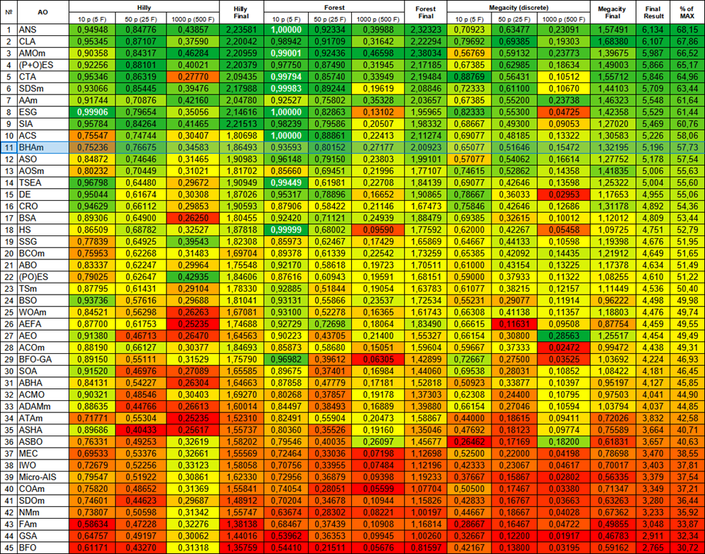
Figure 3. Color gradation of algorithms according to relevant tests Results greater than or equal to 0.99 are highlighted in white
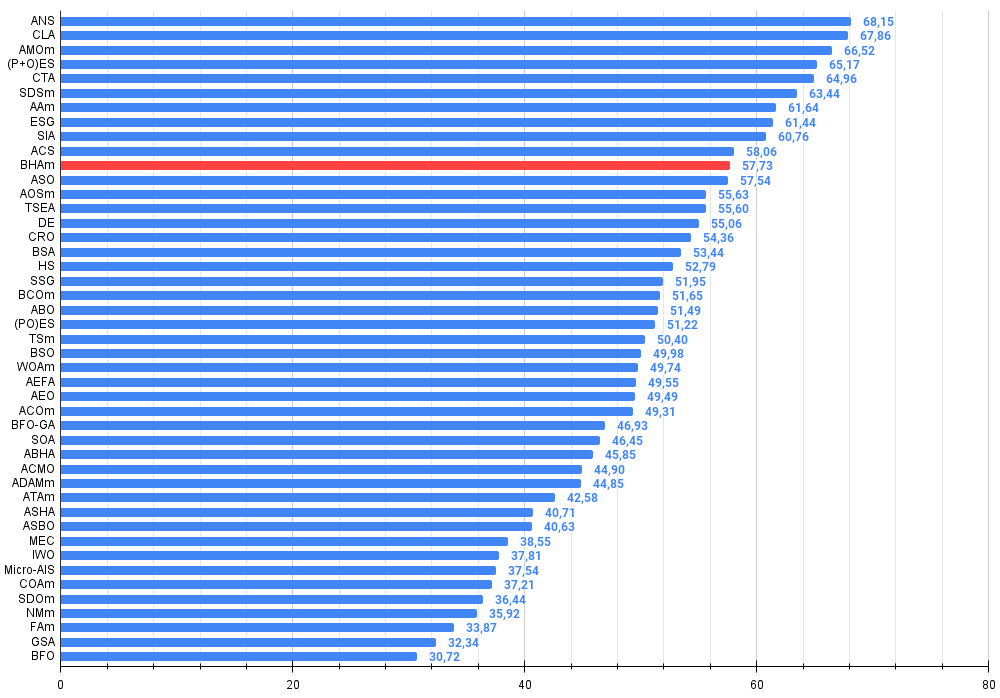
Figure 4. Histogram of algorithm testing results (scale from 0 to 100, the higher the better, where 100 is the maximum possible theoretical result, in the archive there is a script for calculating the rating table)
BHAm pros and cons:
Pros:
- The only external parameter is the population size.
- Simple implementation.
- Very fast EA.
- Works well on large-scale problems.
Disadvantages:
- Large scatter of results on small-dimensional problems.
- Tendency to get stuck on low-dimensional problems.
The article is accompanied by an archive with the current versions of the algorithm codes. The author of the article is not responsible for the absolute accuracy in the description of canonical algorithms. Changes have been made to many of them to improve search capabilities. The conclusions and judgments presented in the articles are based on the results of the experiments.
Programs used in the article
| # | Name | Type | Description |
|---|---|---|---|
| 1 | #C_AO.mqh | Include | Parent class of population optimization algorithms |
| 2 | #C_AO_enum.mqh | Include | Enumeration of population optimization algorithms |
| 3 | TestFunctions.mqh | Include | Library of test functions |
| 4 | TestStandFunctions.mqh | Include | Test stand function library |
| 5 | Utilities.mqh | Include | Library of auxiliary functions |
| 6 | CalculationTestResults.mqh | Include | Script for calculating results in the comparison table |
| 7 | Testing AOs.mq5 | Script | The unified test stand for all population optimization algorithms |
| 8 | Simple use of population optimization algorithms.mq5 | Script | A simple example of using population optimization algorithms without visualization |
| 9 | Test_AO_BHAm.mq5 | Script | BHAm test stand |
Translated from Russian by MetaQuotes Ltd.
Original article: https://www.mql5.com/ru/articles/16655
Warning: All rights to these materials are reserved by MetaQuotes Ltd. Copying or reprinting of these materials in whole or in part is prohibited.
This article was written by a user of the site and reflects their personal views. MetaQuotes Ltd is not responsible for the accuracy of the information presented, nor for any consequences resulting from the use of the solutions, strategies or recommendations described.
 Price Action Analysis Toolkit Development (Part 38): Tick Buffer VWAP and Short-Window Imbalance Engine
 Developing a Replay System (Part 78): New Chart Trade (V)
 Trend strength and direction indicator on 3D bars
 Neural Networks in Trading: A Multi-Agent Self-Adaptive Model (Final Part)
- Free trading apps
- Over 8,000 signals for copying
- Economic news for exploring financial markets
You agree to website policy and terms of use