
MetaTrader 5 Machine Learning Blueprint (Part 7): From Scattered Experiments to Reproducible Results

Introduction
Throughout this series, we've covered crucial components of machine learning for trading: data structures, labeling and meta-labeling, sample weighting and purged cross-validation. But these techniques, powerful as they are individually, reach their full potential only when integrated into a cohesive research system. In this article, I'll demonstrate how to assemble these building blocks into a production-grade pipeline that transforms ad-hoc experiments into reproducible, auditable research and builds on the caching architecture developed in my previous article.
The code we'll explore isn't just another example, it's a major aspect of the system I use for developing trading models. It handles everything from raw tick data to ONNX models ready for deployment in MetaTrader 5, with comprehensive logging, caching, and analysis reports generated automatically along the way. For the sake of clarity, I will ignore some critical topics for now, such as feature importance analysis, and the selection of optimal barriers for the triple-barrier method, among others. This article assumes that these preceding research steps have already occurred, and as such focuses on the creation of reproducible pipelines. What makes a research system "production-grade"?
- Reproducibility: Run the same code twice, get identical results
- Traceability: Know exactly what data trained each model
- Efficiency: Cache expensive computations, never repeat work
- Validation: Catch errors before they reach live trading
- Documentation: Automatic reports that explain every decision

The Problem: Research Chaos
Before we dive into the solution, let's acknowledge the problem. Most trading ML research looks like this:
# Somewhere in notebook cell 47...

df = load_data("EURUSD", "2020-01-01", "2023-12-31")
features = calculate_indicators(df)
X_train, y_train = features[:-1000], labels[:-1000]
model = RandomForestClassifier(n_estimators=100)
model.fit(X_train, y_train)

# Score: 0.67 - is that good? What parameters did I use?
# When did I run this? Which data version?
Three months later, you can't reproduce these results. The data has changed. You don't remember which features you used. The model file has no metadata. You're back to square one.
Not only is this inconvenient, it's dangerous. In live trading, irreproducible research means you can't trust your backtest. You can't debug failures. You can't iterate confidently.
The Solution: A Principled Pipeline
Our research system addresses these problems through four key principles:
- Time-Aware Caching: Never let future data leak into training, but cache everything safely
- Automatic Documentation: Generate comprehensive reports at every stage
- Organized Storage: Navigate your experiments by strategy, symbol, and parameters
- Validation First: Catch errors in research, not in production
Here's the high-level architecture:
Every stage is cached, every decision is logged, every output is validated.
I reiterate, this is a high-level architecture that is in no way meant to cover all steps in the development process.
Intelligent Data Architecture: Why Tick RAM Cache + Parquet Bars Changes Everything
Before we dive into the pipeline stages, let's examine a crucial architectural decision that makes the entire system practical: the data handling strategy.
The Tick Data Dilemma
When developing trading strategies, you face a classic optimization problem:
| Option 1: Load bars directly from broker (MetaTrader 5) | Option 2: Cache everything to disk | Option 3: Hybrid approach (the solution) |
|---|---|---|
|
|
|
Let me show you why this third approach is brilliant.
The TickDataLoader: RAM Caching Done Right
Here's the key insight: tick data should live in RAM, not on disk, because it's the source material you transform in multiple ways. The TickDataLoader class keeps track of all data already loaded in the current session. If we begin our model development with EURUSD data from 2023, and later decide to add 2021-2022 data, only the missing portion is loaded—the cache is extended seamlessly. Instead, TickDataLoader only obtains what was not in the cache and appends it to the preloaded data. The code below is a snippet from the TickDataLoaderclass. For the full code see the attached model_development.py.
class TickDataLoader:
    """
    Loader for tick-level bid/ask data with intelligent local caching.

    Features:
    1. Smart caching that checks if requested date range is within cached ranges
    2. Handles partial overlaps by reusing available cached data
    3. Memory management with cache size limits
    4. Cache statistics tracking

    Notes
    -----
    - Typical performance: ~0.5s for cached retrieval
    - Memory usage: ~100MB per 1M ticks
    """

    def __init__(self, max_cache_size_mb: int = 3000, max_cached_symbols: int = 20):
        """
        Initialize the tick data loader.

        Parameters
        ----------
        max_cache_size_mb : int, optional
            Maximum cache size in MB (default: 5000MB)
        max_cached_symbols : int, optional
            Maximum number of symbols to keep in cache (default: 20)
        """
        self._cache: Dict[Tuple[str, str], pd.DataFrame] = {}  # (symbol, account_name) -> DataFrame
        self._cache_metadata: Dict[Tuple[str, str], Dict] = {}  # (symbol, account_name) -> metadata
        self.max_cache_size_mb = max_cache_size_mb
        self.max_cached_symbols = max_cached_symbols
        self.cache_stats = {
            "hits": 0,
            "misses": 0,
            "partial_hits": 0,
            "total_loaded": 0,
        }

    def get_tick_data(
        self, symbol: str, start_date: str, end_date: str, account_name: str
    ) -> pd.DataFrame:
        """
        Retrieve tick-level bid/ask data with intelligent caching.

        Parameters
        ----------
        symbol : str
            Trading instrument symbol (e.g., 'EURUSD')
        start_date : str
            Start date in 'YYYY-MM-DD' format
        end_date : str
            End date in 'YYYY-MM-DD' format
        account_name : str
            MT5 account identifier for data retrieval

        Returns
        -------
        pd.DataFrame
            Tick data with columns ['bid', 'ask'] indexed by timestamp

        Notes
        -----
        - Checks if cached data fully covers requested date range
        - If partial coverage exists, loads only missing data
        - Merges cached and newly loaded data seamlessly
        """
        cache_key = (symbol, account_name)
        start_dt, end_dt = date_conversion(start_date, end_date)

        # Check if we have cached data for this symbol/account
        if cache_key in self._cache:
            cached_df = self._cache[cache_key]
            metadata = self._cache_metadata[cache_key]
            cached_start, cached_end = date_conversion(metadata["start_date"], metadata["end_date"])

            # Check if cached data fully covers requested range
            if cached_start <= start_dt and cached_end >= end_dt:
                self.cache_stats["hits"] += 1
                logger.debug(f"Cache hit for {symbol} {start_date} to {end_date}")

                # Return subset of cached data
                mask = (cached_df.index >= start_dt) & (cached_df.index <= end_dt)
                return cached_df[mask].copy()

            # Check if there's partial overlap
            if cached_end >= start_dt and cached_start <= end_dt:
                self.cache_stats["partial_hits"] += 1
                logger.debug(f"Partial cache hit for {symbol}")
                return self._load_with_partial_cache(
                    symbol, start_date, end_date, account_name, cache_key
                )

        # No cache hit, load all data
        self.cache_stats["misses"] += 1
        logger.debug(f"Cache miss for {symbol} {start_date} to {end_date}")
        return self._load_and_cache_data(symbol, start_date, end_date, account_name, cache_key)
The system handles three scenarios intelligently:

Below is an example of using the TickDataLoader class:
# Initialize the loader once per session
from ..production.model_development import TickDataLoader

loader = TickDataLoader(
    max_cache_size_mb=3000, # 3GB RAM limit
    max_cached_symbols=20, # Cache up to 20 symbols
)

# First request - loads from disk/MT5 and caches
ticks = loader.get_tick_data(
    symbol="EURUSD",
    start_date="2023-01-01",
    end_date="2023-12-31",
    account_name="FUNDEDNEXT_STLR2_6K"
)
# Takes ~30 seconds (first load)

# Second request - same data, instant from RAM
ticks = loader.get_tick_data(
    symbol="EURUSD",
    start_date="2023-01-01",
    end_date="2023-12-31",
    account_name="FUNDEDNEXT_STLR2_6K"
)
# Takes ~0.5 seconds (cache hit)

# Partial request - subset is instant
ticks = loader.get_tick_data(
    symbol="EURUSD",
    start_date="2023-01-01",
    end_date="2023-03-31",
    account_name="FUNDEDNEXT_STLR2_6K"
)
# Takes ~0.5 seconds (subset from cache)

ticks = loader.get_tick_data(
    symbol="EURUSD",
    start_date="2022-01-01",
    end_date="2023-12-31",
    account_name="FUNDEDNEXT_STLR2_6K"
)
# Takes ~15 seconds (only 2022 data)
And below are features that use tick data:
# Example of features that use tick data

from ..util.volatility import two_time_scale_realized_vol

def two_time_scale_realized_vol(
    tick_prices: pd.Series, slow_freq: str = "5min"
) -> float:
    """
    Two-Time-Scale Realized Volatility Estimator

    Advanced estimator for tick data that removes microstructure noise while
    preserving information. Combines high-frequency and low-frequency sampling
    to extract true volatility signal.

    **What it measures:**
    - True underlying volatility from noisy tick data
    - Removes bid-ask bounce and other microstructure effects
    - Preserves information lost in simple low-frequency sampling

    **Mathematical foundation:**
    - TSRV = RV_slow - (n_slow/n_fast) * (RV_fast - RV_slow)
    - Uses ratio of observation counts to properly scale noise estimate
    - Asymptotically consistent under jump-diffusion models

    **Best used for:**
    - High-frequency trading strategies
    - When you have access to tick data
    - Precision-critical applications (research, risk management)
    - Markets with significant microstructure noise

    **Advantages:**
    - Most accurate volatility estimate for tick data
    - Removes upward bias from microstructure noise
    - Retains more information than sparse sampling
    - Theoretically well-founded

    **Computational considerations:**
    - More intensive than simple realized volatility
    - Requires choice of slow sampling frequency
    - Benefits increase with data quality and frequency

    **Typical slow frequencies:**
    - 1 minute: Very liquid assets, high precision needed
    - 5 minutes: Most common, good noise reduction
    - 15-30 minutes: Less liquid assets

    :param tick_prices: (pd.Series) Tick-level price data, datetime indexed
    :param slow_freq: (str) Slow sampling frequency ('5min', '1min', etc.)
    :return: (float) Two-time-scale realized volatility estimate
    """
    # Fast scale (tick-by-tick)
    tick_returns = np.log(tick_prices / tick_prices.shift(1)).dropna()
    rv_fast = (tick_returns**2).sum()
    n_fast = len(tick_returns)

    # Slow scale (e.g., 5-minute)
    slow_prices = tick_prices.resample(slow_freq).last().dropna()
    slow_returns = np.log(slow_prices / slow_prices.shift(1)).dropna()
    rv_slow = (slow_returns**2).sum()
    n_slow = len(slow_returns)

    # Two-time-scale estimator with proper scaling
    if n_fast > 0 and n_slow > 0:
        tsrv = rv_slow - (n_slow / n_fast) * (rv_fast - rv_slow)
        return max(tsrv, 0)  # Ensure non-negative result
    else:
        return rv_slow


two_time_scale_vol = two_time_scale_realized_vol(tick_prices=ticks["bid"], slow_freq="5min")
Why RAM Instead of Disk?
Think about your typical research workflow:
# You might experiment with:
tick_bars_M1 = make_bars(ticks, "tick", "M1", "mid_price")
tick_bars_M5 = make_bars(ticks, "tick", "M5", "mid_price")
volume_bars = make_bars(ticks, "volume", 1000, "mid_price")
dollar_bars = make_bars(ticks, "dollar", 5000, "mid_price")

# And different price types:
tick_bars_bid = make_bars(ticks, "tick", "M1", "bid")
tick_bars_ask = make_bars(ticks, "tick", "M1", "ask")
You're creating 6 different bar types from the same tick data. If you cached ticks to disk and bars to disk, you'd be storing the same base data multiple times in slightly different aggregations. That's wasteful. You might also decide that you want to create microstructural features (which need tick data). For these reasons, it is best to keep tick data in RAM incase you need it down the road.
Instead:
- Ticks live in RAM (fast access, cleared between sessions)
- Each unique bar configuration gets cached to Parquet (persistent, compact)
- The tick data serves as the "source of truth" for the session
- Parquet files serve as the "compiled artifacts" for long-term storage
The TickDataLoader + Parquet architecture works because it recognizes a fundamental truth about machine learning research:
Raw data should be fast (RAM), processed data should be persistent (Parquet), and you should never duplicate what you can regenerate.
This data architecture scales from individual research to team collaboration. When everyone works with Parquet files, you get:
- Consistent data types (no more "it works on my machine")
- Efficient storage (version control friendly)
- Fast iteration (the cost of experiments approaches zero)
- Reproducibility (Parquet files are binary-stable)
Compare this to CSV-based workflows where you're constantly fighting with:
- Inconsistent date parsing
- Float precision issues
- Encoding problems
- Slow load times
- Large file sizes
- Schema validation headaches
The initial investment in setting up Parquet-based storage pays dividends every single day. And when you combine it with intelligent RAM caching of source data (ticks), you get a system that's both fast and efficient—no compromises necessary.
The Workflow
Let me walk you through a real example: developing a Bollinger Band reversal strategy for EURUSD. We'll see exactly what happens at each stage and what artifacts get generated.
Stage 1: Configuration
Everything starts with configuration. Not scattered parameters across multiple files, but a single source of truth:
from model_development import ModelDevelopmentPipeline
from strategies import BollingerBandStrategy

# Data configuration
data_config = {
    "symbol": "EURUSD",
    "train_start": "2023-01-01",
    "train_end": "2023-12-31",
    "account_name": "FUNDEDNEXT_STLR2_6K",
    "bar_type": "tick",
    "bar_size": "M1",  # Will be converted to tick count
    "price": "mid_price"
}

# Feature configuration
feature_config = {
    "func": calculate_bollinger_features,
    "params": {
        "window": 20,
        "num_std": 2.0
    }
}

# Triple-barrier labeling
target_config = {
    "func": get_daily_vol,
    "params": {"lookback": 20}
}

label_config = {
    "profit_target": 1.0,
    "stop_loss": 2.0,
    "max_holding_period": {"days": 1},
    "min_ret": 0.0,
    "vertical_barrier_zero": True,
    "filter_as_series": False
}

# Model training parameters
model_params = {
    "pipe_clf": RandomForestClassifier(
        criterion="entropy",
        class_weight="balanced_subsample",
        min_weight_fraction_leaf=0.05
    ),
    "param_grid": {
        "n_estimators": [100, 200, 300],
        "max_depth": [3, 5, 7, 10],
        "min_samples_split": [2, 5, 10]
    },
    "cv_splits": 5,
    "bagging_n_estimators": 10,
    "n_jobs": -1,
    "random_state": 42
}

# Initialize strategy
strategy = BollingerBandStrategy(
    window=20,
    std=2.0,
)
Notice how every parameter is explicit and documented. Three months from now, you'll know exactly what you did.
Stage 2: Pipeline Initialization
Now we create the pipeline with intelligent file management:
pipeline = ModelDevelopmentPipeline(
    strategy=strategy,
    data_config=data_config,
    feature_config=feature_config,
    target_config=target_config,
    label_config=label_config,
    model_params=model_params,
    base_dir="Models"
)
Behind the scenes, this creates a structured directory: Models/ └── BollingerBandStrategy/ └── EURUSD/ └── FUNDEDNEXT_STLR2_6K/ └── tick/ └── M1/ └── 20230101_20231231/ └── a3f7b2e9/ # Config hash ├── config.json ├── logs/ ├── plots/ └── reports/Every configuration gets its own directory. No more "model_v2_final_REALLY_FINAL.pkl".
Stage 3: Execution
With configuration complete, we run the entire pipeline:
model, features, metrics, config = pipeline.run(
    generate_reports=True,
    save=True,
    export_onnx=True,
    verbose=True
)
Now the magic happens. Let's see what occurs at each stage:
Step 1: Data Loading (with Smart Caching)
[Step 1/7] Loading training data...
✓ Cache hit for EURUSD 2023-01-01 to 2023-12-31
✓ Retrieved 15,847,392 ticks in 0.4s
✓ Constructed 262,800 M1 bars
The system checks if we've already loaded this data. If so, it's retrieved from cache in milliseconds rather than minutes. But here's the crucial part: the caching is time-aware. It tracks what data was accessed when, preventing future data from leaking into your training set.
# From model_development.py
@cacheable(time_aware=True)
def load_and_prepare_training_data(symbol, start_date, end_date, ...):
    tick_df = loader.get_tick_data(symbol, start_date, end_date, account_name)
    data = make_bars(tick_df, bar_type, bar_size, price)

    # Log data access for contamination tracking
    log_data_access(
        dataset_name=f"{symbol}_{bar_type}_{bar_size}_{price}".lower(),
        start_date=data.index[0],
        end_date=data.index[-1],
        purpose="train"
    )

    return data
Step 2: Feature Engineering
✓ Generated 47 features
- 12 Bollinger Band features
- 15 momentum features
- 8 volume features
- 12 time-based features
@cacheable(time_aware=True)
def create_feature_engineering_pipeline(data, feature_config, data_config):
    func = feature_config["func"]
    features = func(data, **feature_config["params"])
    time_feat = get_time_features(data, timeframe=data_config["bar_size"])
    return features.join(time_feat).dropna()
If your feature function changes, the cache automatically invalidates. If only the data changes, features are recomputed efficiently.
Step 3: Label Generation
[Step 3/7] Generating events...
✓ Generated 89,247 events
✓ Label distribution:
- Long (1): 38,562 (43.2%)
- None (0): 24,891 (27.9%)
- Short (-1): 25,794 (28.9%)
@cacheable()
def generate_events_triple_barrier(data, strategy, target_config,
                                   profit_target, stop_loss, ...):
    # Calculate dynamic barriers based on volatility
    close = data["close"]
    fn = target_config["func"]
    params = target_config["params"]
    target = fn(close, **params)

    # Get entry signals from strategy
    side, t_events = get_entries(strategy, data, target.mean())

    # Apply triple-barrier method
    vb = add_vertical_barrier(t_events, close, **max_holding_period)
    events = triple_barrier_labels(close, target, t_events,
                                   vertical_barrier_times=vb,
                                   side_prediction=side,
                                   pt_sl=[profit_target, stop_loss], ...)

    # Add sample weights
    events = get_event_weights(events, close)
    return events
Step 4: Sample Weight Optimization
Here's where it gets interesting. Rather than guessing at sample weights, we search for the optimal weighting scheme:
Testing weighting schemes:
- unweighted + linear decay
- unweighted + exponential decay
- return-based + linear decay
- return-based + exponential decay
- uniqueness + linear decay
- uniqueness + exponential decay
✓ Best scheme: uniqueness_linear_0.7428 (CV Score: 0.6847)
The system tries multiple weighting approaches and picks the one that performs best on purged cross-validation:
@cacheable()
def get_optimal_sample_weight(
    data_index: pd.DatetimeIndex,
    events: pd.DataFrame,
    features: pd.DataFrame,
    cv_splits: int = 5,
    n_iter: int = 10,
) -> pd.Series:
    """
    Compute best sample weight with time decay.

    Parameters
    ----------
    data_index: pd.DatetimeIndex
        Price data index.
    events : pd.DataFrame
        Event labels with uniqueness weights.
    features: pd.DataFrame
        Training features
    cv_splits : int, optional
        Number of cross-validation splits (default: 5).
    n_iter : int, optional
        Number of random search iterations (default: 10).

    Returns
    -------
    weights : pd.Series
        Computed sample weights.
    cv_results : dict
        Cross-validation results.
    """
    valid_index = features.index.intersection(events.index)
    cont = events.loc[valid_index]
    X = features.loc[valid_index]
    y = cont["bin"]

    classifier = RandomForestClassifier(
        criterion="entropy",
        class_weight="balanced_subsample",
        max_samples=cont["tW"].mean(),
        max_depth=4,
        min_weight_fraction_leaf=0.05,
    )
    scoring = "f1" if set(y.unique()) == {0, 1} else "neg_log_loss"
    cv_gen = PurgedKFold(n_splits=cv_splits, t1=cont["t1"], pct_embargo=0.02)
    weights = [
        ("return", cont["w"]),
        ("unweighted", pd.Series(1.0, index=cont.index)),
        ("uniqueness", cont["tW"]),
    ]
    best_score = 0
    cv_results = pd.DataFrame()

    for scheme, weight in tqdm(weights, desc="Analyzing weighting schemes", total=len(weights)):
        scores = ml_cross_val_score(
            classifier,
            X,
            y,
            cv_gen,
            sample_weight_train=weight,
            sample_weight_score=weight,
            scoring=scoring,
        )
        score = scores.mean()
        cv_results[scheme] = scores

        if not np.isinf(score) and score > best_score:
            best_score = score
            best_weight = weight
            best_scheme = scheme

    est = weighted_estimator(classifier, cont, data_index)
    param_distributions = {
        "scheme": [best_scheme],
        "decay": uniform(0, 1),  # decay factor between 0 and 1 inclusive
        "linear": [True, False],
    }
    gs = RandomizedSearchCV(
        estimator=est,
        param_distributions=param_distributions,
        n_iter=n_iter,
        cv=cv_gen,
        scoring=scoring,
        n_jobs=-1,
        random_state=42,
        refit=False,
    )
    gs.fit(X, y)

    scheme, decay, linear = [gs.best_params_[k] for k in ["scheme", "decay", "linear"]]
    best_scheme = f"{scheme}_{'linear' if linear else 'exp'}_{decay}"
    logger.info(f"Best sample weight scheme: {best_scheme}")

    decay_vec = get_weights_by_time_decay_optimized(
        triple_barrier_events=cont,
        close_index=data_index,
        last_weight=decay,
        linear=linear,
        av_uniqueness=cont["tW"],
    )

    best_weight *= decay_vec

    cv_results = {
        "best_score": best_score,
        "cv_results_scheme": cv_results,
        "cv_results": pd.DataFrame(gs.cv_results_),
        "scoring": scoring,
        "best_scheme": best_scheme,
    }

    return best_weight, cv_results
In this manner, you discover which weighting scheme actually helps your specific strategy.
Step 5: Meta-Features
✓ Added 8 meta-features
- rolling_accuracy_20, rolling_accuracy_50
- rolling_precision_20, rolling_precision_50
- rolling_recall_20, rolling_recall_50
- rolling_f1_20, rolling_f1_50
These features tell the model how well it's been doing recently, which can improve meta-labeling performance. The calculation is optimized with Numba for speed:
@njit(parallel=True, fastmath=True, cache=True)
def _rolling_metrics_numba(y_true, y_pred, weights, window):
    """Numba-accelerated rolling metrics calculation."""
    n = len(y_true)
    accuracy = np.full(n, np.nan)
    precision = np.full(n, np.nan)
    recall = np.full(n, np.nan)
    f1 = np.full(n, np.nan)

    for i in prange(window - 1, n):
        start = i - window + 1
        tp = fp = tn = fn = 0.0

        # Inner loop for window
        for j in range(start, i + 1):
            if y_true[j] == 1 and y_pred[j] == 1:
                tp += weights[j]
            elif y_true[j] == 0 and y_pred[j] == 1:
                fp += weights[j]
            elif y_true[j] == 0 and y_pred[j] == 0:
                tn += weights[j]
            elif y_true[j] == 1 and y_pred[j] == 0:
                fn += weights[j]

        total = tp + fp + tn + fn
        if total > 0:
            accuracy[i] = (tp + tn) / total

        denom_prec = tp + fp
        if denom_prec > 0:
            precision[i] = tp / denom_prec

        denom_rec = tp + fn
        if denom_rec > 0:
            recall[i] = tp / denom_rec

        if not np.isnan(precision[i]) and not np.isnan(recall[i]):
            denom_f1 = precision[i] + recall[i]
            if denom_f1 > 0:
                f1[i] = 2 * (precision[i] * recall[i]) / denom_f1

    return accuracy, precision, recall, f1
Step 6: Model Training with Hyperparameter Search
This is the heart of the system—intelligent hyper-parameter optimization with proper cross-validation:
[Step 6/7] Training model with cross-validation...
Grid Search Progress: Testing 81 parameter combinations
Using 5-fold purged cross-validation
Embargo: 1% between folds
[████████████████████████████████████] 81/81 (100%)
✓ Best parameters found:
- n_estimators: 200
- max_depth: 7
- min_samples_split: 5
✓ Cross-validation scores:
- Mean F1: 0.6847 ± 0.0234
- Fold 0: 0.6923
- Fold 1: 0.6801
- Fold 2: 0.6889
- Fold 3: 0.6712
- Fold 4: 0.6912
✓ Training bagged ensemble (10 estimators)...
✓ Model training complete
The hyper-parameter search uses purged k-fold cross-validation to prevent leakage:
def train_model_with_cv(
    features: pd.DataFrame,
    events: pd.DataFrame,
    sample_weight: np.ndarray,
    pipe_clf: Union[ClassifierMixin, Pipeline],
    param_grid: Dict,
    cv_splits: int = 5,
    bagging_n_estimators: int = 0,
    bagging_max_samples: float = 1.0,
    bagging_max_features: float = 1.0,
    rnd_search_iter: int = 0,
    n_jobs: int = -1,
    pct_embargo: float = 0.02,
    random_state: int = None,
    verbose: int = 0,
) -> Tuple[RandomForestClassifier, Dict]:
    """
    Train model with cross-validation using cached hyperparameter search.

    Parameters
    ----------
    features : pd.DataFrame
        Feature matrix.
    events : pd.DataFrame
        Event labels.
    sample_weight : np.ndarray
        Sample weights aligned with events.
    pipe_clf : sklearn.Pipeline
        Pipeline including classifier.
    param_grid : dict
        Hyperparameter grid for search.
    cv_splits : int, default=5
        Number of CV splits.
    bagging_n_estimators : int, default=0
        Number of bagging estimators.
    bagging_max_samples : float, default=1.0
        Max samples for bagging.
    bagging_max_features : float, default=1.0
        Max features for bagging.
    rnd_search_iter : int, default=0
        Randomized search iterations.
    n_jobs : int, default=-1
        Parallel jobs.
    pct_embargo : float, default=0.02
        Embargo percentage for purging CV splits.
    random_state : int, optional
        Random seed.
    verbose : int, default=0
        Verbosity flag.

    Returns
    -------
    best_model : RandomForestClassifier
        Trained best model.
    cv_results : dict
        Cross-validation results.

    """
    valid_index = features.index.intersection(events.index)
    cont = events.loc[valid_index]
    X = features.loc[valid_index]
    y = cont["bin"]
    t1 = cont["t1"]
    w = sample_weight.loc[valid_index]

    best_model, cv_results = clf_hyper_fit(
        features=X,
        labels=y,
        t1=t1,
        pipe_clf=pipe_clf,
        param_grid=param_grid,
        cv=cv_splits,
        bagging_n_estimators=bagging_n_estimators,
        bagging_max_samples=bagging_max_samples,
        bagging_max_features=bagging_max_features,
        rnd_search_iter=rnd_search_iter,
        n_jobs=n_jobs,
        pct_embargo=pct_embargo,
        random_state=random_state,
        verbose=verbose,
        sample_weight=w,
    )

    return best_model, cv_results
- Performance distribution across all parameter combinations
- Score vs stability scatter plot
- Score vs training time analysis
- Parameter importance rankings
- Cross-validation fold consistency
Step 7: Feature Importance Analysis
[Step 7/7] Analyzing feature importance...
2025-12-16 11:18:21 [info     ] pipeline_step                  duration_seconds=0.1509995460510254 metrics={'top_feature': 'rolling_accuracy_20'} status=completed step=feature_analysis

Top 10 Features:
            feature  importance
rolling_accuracy_20    0.166330
      rolling_f1_20    0.132372
rolling_accuracy_50    0.131260
      rolling_f1_50    0.109463
             spread    0.029035
             d1_vol    0.025773
        hour_cos_h2    0.022493
        ret_1_lag_1    0.022391
   parkinson_vol_10    0.019278
 london_session_vol    0.018018
Feature importance helps us understand what the model learned and identify potential issues.
Stage 4: Automated Report Generation
After training completes, the system automatically generates comprehensive analysis reports. This is what the output after completion looks like:
2025-12-16 11:14:08 | afml.production.model_development | INFO | Starting pipeline for EURUSD
2025-12-16 11:14:08 | afml.production.model_development | INFO | Training period: 2022-01-01 to 2023-12-31
2025-12-16 11:14:08 | afml.production.model_development | INFO | Output directory: Models\Bollinger_w10_std1_5\EURUSD\FUNDEDNEXT_STLR2_6K\time\M1\20220101_20231231\bdad004f

======================================================================
PRODUCTION MODEL DEVELOPMENT PIPELINE
======================================================================

Configuration
--------------------------------------------------
strategy                 Bollinger_w10_std1.5
symbol                                 EURUSD
training_start                     2022-01-01
training_end                       2023-12-31
account_name              FUNDEDNEXT_STLR2_6K
bar_type                                 time
bar_size                                   M1
price                               mid_price
target_lookback                            10
profit_target                               1
stop_loss                                   2
max_holding_period                {'days': 1}
min_ret                                     0
vertical_barrier_zero                    True
filter_as_series                        False
2025-12-16 11:14:09 [info     ] pipeline_step                  status=started step=pipeline_start strategy=Bollinger_w10_std1.5 symbol=EURUSD train_period=2022-01-01_2023-12-31

[Step 1/7] Loading training data...
2025-12-16 11:14:09 | afml.cache.unified_cache_system | DEBUG | Cache HIT: afml.production.model_development.load_and_prepare_training_data (key: d890725d...)
2025-12-16 11:14:09 [info     ] pipeline_step                  duration_seconds=0.10399937629699707 metrics={'samples': 738824} status=completed step=data_loading
✓ Loaded 738,824 samples

[Step 2/7] Computing features...
2025-12-16 11:14:09 | afml.cache.unified_cache_system | DEBUG | Cache HIT: afml.production.model_development.create_feature_engineering_pipeline (key: 4e32ea77...)
2025-12-16 11:14:09 [info     ] pipeline_step                  duration_seconds=0.699995756149292 metrics={'features_generated': 68} status=completed step=feature_engineering
✓ Generated 68 features

[Step 3/7] Generating events...
2025-12-16 11:14:09 | afml.cache.unified_cache_system | DEBUG | Cache HIT: afml.production.model_development.generate_events_triple_barrier (key: 5a7b1eb0...)
2025-12-16 11:14:09 [info     ] pipeline_step                  duration_seconds=0.14899849891662598 metrics={'events_generated': 75975, 'label_distribution':       count  proportion
bin
1    49,791     0.65536
0    26,184     0.34464, 'average_uniqueness': 0.4667911271632548} status=completed step=label_generation
✓ Generated events:
      count  proportion
bin
1    49,791     0.65536
0    26,184     0.34464

Average Uniqueness: 0.4668

[Step 4/7] Computing sample weights...
2025-12-16 11:18:04 | afml.production.model_development | INFO | Best Weighting Scheme: Uniqueness Exp 0.05808
2025-12-16 11:18:07 | afml.cache.unified_cache_system | DEBUG | Cache MISS: afml.production.model_development.find_optimal_sample_weight (key: 9d10ce42...) (00:03:57)
2025-12-16 11:18:07 [info     ] pipeline_step                  duration_seconds=237.31548690795898 metrics={'weighting_scheme': 'uniqueness_exp_0.05808361216819946', 'weight_cv_score': 0.7457131539000748} status=completed step=weight_computation
✓ Best weighting scheme: uniqueness_exp_0.05808361216819946

[Step 5/7] Computing rolling meta-label features...
2025-12-16 11:18:07 | afml.cache.unified_cache_system | DEBUG | Cache HIT: afml.production.model_development.calculate_rolling_metrics (key: ae8cdce2...)
2025-12-16 11:18:20 [info     ] pipeline_step                  duration_seconds=13.350001573562622 metrics={'meta_features_added': 8, 'features_after_preprocessing': 72, 'features_removed': -4} status=completed step=meta_features_preprocessing
✓ Computed rolling meta-label features
✓ Preprocessed features: 72 features retained

[Step 6/7] Training model with cross-validation...
2025-12-16 11:18:21 | afml.cache.unified_cache_system | DEBUG | Cache HIT: afml.cross_validation.hyper_fit.clf_hyper_fit_internal (key: 907bd2af...)
2025-12-16 11:18:21 [info     ] pipeline_step                  duration_seconds=0.4719998836517334 metrics={'cv_score': 0.6915768921130778, 'best_params': {'clf__max_depth': 6, 'clf__max_features': 0.12075618253727419, 'clf__min_samples_leaf': 3, 'clf__min_samples_split': 13, 'clf__min_weight_fraction_leaf': 0.28140549728612524, 'clf__n_estimators': 369}, 'n_splits': 5} status=completed step=model_training
✓ Best CV score: 0.6916
✓ Best params: {'clf__max_depth': 6, 'clf__max_features': 0.12075618253727419, 'clf__min_samples_leaf': 3, 'clf__min_samples_split': 13, 'clf__min_weight_fraction_leaf': 0.28140549728612524, 'clf__n_estimators': 369}

[Step 7/7] Analyzing feature importance...
2025-12-16 11:18:21 [info     ] pipeline_step                  duration_seconds=0.1509995460510254 metrics={'top_feature': 'rolling_accuracy_20'} status=completed step=feature_analysis

Top 10 Features:
            feature  importance
rolling_accuracy_20    0.166330
      rolling_f1_20    0.132372
rolling_accuracy_50    0.131260
      rolling_f1_50    0.109463
             spread    0.029035
             d1_vol    0.025773
        hour_cos_h2    0.022493
        ret_1_lag_1    0.022391
   parkinson_vol_10    0.019278
 london_session_vol    0.018018


[Generating Reports] Creating analysis reports...
🔍 Running hyperparameter analysis...
================================================================================
HYPERPARAMETER ANALYSIS REPORT
================================================================================

1. TOP PERFORMING MODELS (sorted by mean_test_score):
--------------------------------------------------
                                                                                                                                                                                                       params  mean_test_score  std_test_score  mean_fit_time
4   {'clf__max_depth': 6, 'clf__max_features': 0.12075618253727419, 'clf__min_samples_leaf': 3, 'clf__min_samples_split': 13, 'clf__min_weight_fraction_leaf': 0.28140549728612524, 'clf__n_estimators': 369}         0.691577        0.011027      28.989994
2    {'clf__max_depth': 4, 'clf__max_features': 0.15077042112439024, 'clf__min_samples_leaf': 8, 'clf__min_samples_split': 13, 'clf__min_weight_fraction_leaf': 0.4723487190570876, 'clf__n_estimators': 435}         0.683852        0.011899      28.105996
6    {'clf__max_depth': 4, 'clf__max_features': 0.9539969835279999, 'clf__min_samples_leaf': 2, 'clf__min_samples_split': 10, 'clf__min_weight_fraction_leaf': 0.05718481349909639, 'clf__n_estimators': 435}         0.677322        0.006976     614.569299
17    {'clf__max_depth': 4, 'clf__max_features': 0.8984914683186939, 'clf__min_samples_leaf': 1, 'clf__min_samples_split': 4, 'clf__min_weight_fraction_leaf': 0.10381741067223577, 'clf__n_estimators': 180}         0.675696        0.006911     175.406800
1     {'clf__max_depth': 5, 'clf__max_features': 0.5133240027692805, 'clf__min_samples_leaf': 5, 'clf__min_samples_split': 5, 'clf__min_weight_fraction_leaf': 0.11429006806487335, 'clf__n_estimators': 180}         0.670490        0.007110      95.500397
5     {'clf__max_depth': 3, 'clf__max_features': 0.14180537144799796, 'clf__min_samples_leaf': 3, 'clf__min_samples_split': 8, 'clf__min_weight_fraction_leaf': 0.1267358556592812, 'clf__n_estimators': 216}         0.669676        0.009235      33.474998
10    {'clf__max_depth': 4, 'clf__max_features': 0.905344615384884, 'clf__min_samples_leaf': 8, 'clf__min_samples_split': 15, 'clf__min_weight_fraction_leaf': 0.13819228808861533, 'clf__n_estimators': 239}         0.669449        0.008087     196.870216
16    {'clf__max_depth': 4, 'clf__max_features': 0.1858691048413702, 'clf__min_samples_leaf': 7, 'clf__min_samples_split': 6, 'clf__min_weight_fraction_leaf': 0.37832278025212884, 'clf__n_estimators': 409}         0.667428        0.007923      36.593196
13   {'clf__max_depth': 5, 'clf__max_features': 0.4810613326357327, 'clf__min_samples_leaf': 1, 'clf__min_samples_split': 13, 'clf__min_weight_fraction_leaf': 0.18206967862311718, 'clf__n_estimators': 112}         0.664284        0.002792      40.329997
12   {'clf__max_depth': 3, 'clf__max_features': 0.3528410587186427, 'clf__min_samples_leaf': 9, 'clf__min_samples_split': 16, 'clf__min_weight_fraction_leaf': 0.12437012257835113, 'clf__n_estimators': 394}         0.664078        0.007689     133.290791

2. PERFORMANCE SUMMARY:
--------------------------------------------------
Average mean_test_score: 0.6656 ± 0.0106
Best mean_test_score: 0.6916
Worst mean_test_score: 0.6482
Performance Range: 0.0434

3. STABILITY ANALYSIS:
--------------------------------------------------
Models with stable performance (std ≤ 0.03): 20
Best stable model: 0.6916 ± 0.0110

4. TIME-EFFICIENCY ANALYSIS:
--------------------------------------------------

5. HYPERPARAMETER TRENDS:
--------------------------------------------------

Parameter: clf__max_depth
Optimal value: 4 (score: 0.6716)
Performance by value:
                      score_mean  score_std  count  fold_std_mean  time_mean
param_clf__max_depth
4                         0.6716     0.0098      6         0.0088   184.0137
6                         0.6659     0.0177      4         0.0104    99.7223
3                         0.6638     0.0048      4         0.0088   108.2067
5                         0.6607     0.0073      6         0.0076    60.1069

Parameter: clf__max_features
Optimal value: 0.12075618253727419 (score: 0.6916)
Performance by value:
                         score_mean  score_std  count  fold_std_mean  time_mean
param_clf__max_features
0.120756                     0.6916        NaN      1         0.0110    28.9900
0.150770                     0.6839        NaN      1         0.0119    28.1060
0.953997                     0.6773        NaN      1         0.0070   614.5693
0.898491                     0.6757        NaN      1         0.0069   175.4068
0.513324                     0.6705        NaN      1         0.0071    95.5004
0.141805                     0.6697        NaN      1         0.0092    33.4750
0.905345                     0.6694        NaN      1         0.0081   196.8702
0.185869                     0.6674        NaN      1         0.0079    36.5932
0.481061                     0.6643        NaN      1         0.0028    40.3300
0.352841                     0.6641        NaN      1         0.0077   133.2908
0.749557                     0.6636        NaN      1         0.0093   166.1914
0.316923                     0.6623        NaN      1         0.0069   119.1400
0.484787                     0.6620        NaN      1         0.0052    37.7866
0.816889                     0.6600        NaN      1         0.0078   117.2920
0.278958                     0.6595        NaN      1         0.0110    46.2450
0.860080                     0.6581        NaN      1         0.0081   132.6173
0.933671                     0.6579        NaN      1         0.0089    99.8698
0.568061                     0.6556        NaN      1         0.0112    52.5364
0.992990                     0.6515        NaN      1         0.0156   118.1418
0.918388                     0.6482        NaN      1         0.0115    23.4877

Parameter: clf__min_samples_leaf
Optimal value: 3 (score: 0.6744)
Performance by value:
                             score_mean  score_std  count  fold_std_mean  time_mean
param_clf__min_samples_leaf
3                                0.6744     0.0153      3         0.0085    33.4172
5                                0.6705        NaN      1         0.0071    95.5004
8                                0.6682     0.0114      4         0.0097    97.1283
2                                0.6677     0.0136      2         0.0076   373.5933
7                                0.6644     0.0027      3         0.0081   107.3082
1                                0.6638     0.0121      3         0.0084   111.2929
9                                0.6610     0.0044      2         0.0083   116.5803
4                                0.6519     0.0052      2         0.0113    38.0120

Parameter: clf__min_samples_split
Optimal value: 10 (score: 0.6773)
Performance by value:
                              score_mean  score_std  count  fold_std_mean  time_mean
param_clf__min_samples_split
10                                0.6773        NaN      1         0.0070   614.5693
13                                0.6707     0.0165      5         0.0097    66.9416
5                                 0.6705        NaN      1         0.0071    95.5004
4                                 0.6676     0.0115      2         0.0090   110.8259
6                                 0.6674        NaN      1         0.0079    36.5932
15                                0.6665     0.0041      2         0.0087   181.5308
8                                 0.6624     0.0051      4         0.0078    72.1058
16                                0.6611     0.0042      2         0.0079   132.9540
19                                0.6519     0.0052      2         0.0113    38.0120

Parameter: clf__min_weight_fraction_leaf
Optimal value: 0.28140549728612524 (score: 0.6916)
Performance by value:
                                     score_mean  score_std  count  fold_std_mean  time_mean
param_clf__min_weight_fraction_leaf
0.281405                                 0.6916        NaN      1         0.0110    28.9900
0.472349                                 0.6839        NaN      1         0.0119    28.1060
0.057185                                 0.6773        NaN      1         0.0070   614.5693
0.103817                                 0.6757        NaN      1         0.0069   175.4068
0.114290                                 0.6705        NaN      1         0.0071    95.5004
0.126736                                 0.6697        NaN      1         0.0092    33.4750
0.138192                                 0.6694        NaN      1         0.0081   196.8702
0.378323                                 0.6674        NaN      1         0.0079    36.5932
0.182070                                 0.6643        NaN      1         0.0028    40.3300
0.124370                                 0.6641        NaN      1         0.0077   133.2908
0.272208                                 0.6636        NaN      1         0.0093   166.1914
0.272830                                 0.6623        NaN      1         0.0069   119.1400
0.263917                                 0.6620        NaN      1         0.0052    37.7866
0.250625                                 0.6600        NaN      1         0.0078   117.2920
0.405579                                 0.6595        NaN      1         0.0110    46.2450
0.422932                                 0.6581        NaN      1         0.0081   132.6173
0.432517                                 0.6579        NaN      1         0.0089    99.8698
0.398810                                 0.6556        NaN      1         0.0112    52.5364
0.325244                                 0.6515        NaN      1         0.0156   118.1418
0.348135                                 0.6482        NaN      1         0.0115    23.4877

6. CROSS-VALIDATION CONSISTENCY:
--------------------------------------------------
Fold performance consistency:
  Fold 0: 0.6758 ± 0.0113
  Fold 1: 0.6734 ± 0.0104
  Fold 2: 0.6607 ± 0.0091
  Fold 3: 0.6612 ± 0.0127
  Fold 4: 0.6570 ± 0.0149

7. MODEL SELECTION RECOMMENDATION:
--------------------------------------------------
✅ RECOMMENDATION: Choose stable model
   Score: 0.6916 (vs best: 0.6916)
   Stability: 0.0110 (vs best: 0.0110)
   Performance difference: 0.0000 (insignificant)

🎯 RECOMMENDED HYPERPARAMETERS:
   clf__max_depth: 6
   clf__max_features: 0.12075618253727419
   clf__min_samples_leaf: 3
   clf__min_samples_split: 13
   clf__min_weight_fraction_leaf: 0.28140549728612524
   clf__n_estimators: 369

8. GENERATING VISUALIZATIONS...

9. PRACTICAL INTERPRETATION FOR TRADING:
--------------------------------------------------
Expected Strategy Performance:
  • Best mean_test_score: 0.6916
  • Cross-validation Consistency: Good

✅ LOW RISK: Excellent consistency across CV folds
   Strategy likely to perform similarly in live trading

================================================================================
ANALYSIS COMPLETE
================================================================================
SPECIFIC INSIGHTS FROM YOUR RESULTS:
================================================================================

1. KEY OBSERVATIONS:
--------------------------------------------------
max_depth: 6
min_samples_leaf: 3
min_samples_split: 13
n_estimators: 369
Best Model mean_test_score: 0.6916
Standard Deviation: 0.0110
Training Time: 28.99s

Best Simple Model (param_clf__max_depth ≤ 4):
  param_clf__max_depth=4
  mean_test_score: 0.6839 (vs best: 0.6916)

2. PERFORMANCE SATURATION:
--------------------------------------------------
Maximum performance by max_depth:
  depth=3: 0.6697
  depth=4: 0.6839
  depth=5: 0.6705
  depth=6: 0.6916

3. ACTIONABLE RECOMMENDATIONS:
--------------------------------------------------
✅ Excellent performance achieved!
   Consider testing with additional features or ensemble methods

4. PRODUCTION CONSIDERATIONS:
--------------------------------------------------
Expected Inference Speed: ~199.1ms per prediction
Training Time Range: 23.49s to 614.57s
Average Model Size: ~303 trees
✅ Markdown report generated: Models\Bollinger_w10_std1_5\EURUSD\FUNDEDNEXT_STLR2_6K\time\M1\20220101_20231231\bdad004f\reports\hyperparameter_analysis_report.md
2025-12-16 11:18:24 | afml.production.model_development | INFO | Generated hyperparameter report: Models\Bollinger_w10_std1_5\EURUSD\FUNDEDNEXT_STLR2_6K\time\M1\20220101_20231231\bdad004f\reports\hyperparameter_analysis_report.md
2025-12-16 11:18:25 | afml.production.model_development | INFO | Generated feature importance plot: Models\Bollinger_w10_std1_5\EURUSD\FUNDEDNEXT_STLR2_6K\time\M1\20220101_20231231\bdad004f\plots\feature_importance.png
2025-12-16 11:18:25 | afml.production.model_development | WARNING | HTML summary generation failed: 'numpy.ndarray' object is not callable
✓ Reports generated in 4.15s

[Saving] Writing artifacts to disk...
2025-12-16 11:18:29 | afml.production.model_development | INFO | Saved all artifacts to Models\Bollinger_w10_std1_5\EURUSD\FUNDEDNEXT_STLR2_6K\time\M1\20220101_20231231\bdad004f
✓ Saved to Models\Bollinger_w10_std1_5\EURUSD\FUNDEDNEXT_STLR2_6K\time\M1\20220101_20231231\bdad004f
2025-12-16 11:18:29 [info     ] pipeline_step                  duration_seconds=260.72733187675476 metrics={'total_duration': 260.72733187675476, 'model_trained': True, 'reports_generated': True} status=completed step=pipeline_complete

✓ Pipeline completed in 00:04:21
======================================================================
Stage 5: Model Export and Validation
The final stage exports the model to ONNX format with comprehensive validation:
[Saving] Writing artifacts to disk... ONNX EXPORT PIPELINE

======================================================================
ONNX EXPORT PIPELINE
======================================================================

[Step 1/5] Preparing metadata...
✓ Model type: RandomForestClassifier
✓ Features: 74
✓ Version: 1.0

[Step 2/5] Converting to ONNX format...
✓ Conversion successful
✓ ONNX opset: 12 (MQL5 compatible)

[Step 3/5] Saving ONNX model...
✓ Saved to: C:\Users\JoeN\Documents\GitHub\Machine-Learning-Blueprint\models\bollinger_meta_model_eurusd_tick_m1.onxx
✓ File size: 0.16 MB

[Step 4/5] Validating ONNX model...
✓ ONNX model structure valid

[Step 5/5] Comparing Python vs ONNX predictions...

Generating test data...
Computing Python predictions...
Computing ONNX predictions...

✓ ONNX returned 2 output(s)
  Output 0: shape=(1000,), dtype=int64
    Sample values: 1
  Output 1: shape=(1000, 2), dtype=float32
    Sample values: [0.48720157 0.5127984 ]

✓ Using output 1 (probabilities)
✓ Extracted positive class probabilities from shape (1000, 2)

Prediction Comparison (1000 samples):
  • Max difference:  1.52e-07
  • Mean difference: 4.91e-08
  • Std difference:  3.30e-08

✅ VALIDATION PASSED - Predictions match within tolerance (1.00e-05)

Sample Predictions (first 5):
Index    Python       ONNX         Diff
--------------------------------------------------
0        0.512798     0.512798     8.19e-08
1        0.459688     0.459688     5.50e-08
2        0.451748     0.451748     7.06e-08
3        0.478857     0.478857     6.04e-08
4        0.460223     0.460223     6.36e-08

======================================================================
✅ EXPORT SUCCESSFUL - Model ready for MQL5 deployment
======================================================================
This validation step is crucial. The system generates random test data and verifies that the ONNX model produces bit-for-bit identical predictions to the Python model. If there's any discrepancy, the export fails immediately rather than silently producing wrong predictions in production.
Understanding the Outputs
After the pipeline completes, you have a complete audit trail. Every file is timestamped, versioned, and linked. You can navigate your research history like a well-organized library.

| File Types (Color as Key) | Function |
|---|---|
| Configuration Files | Complete settings needed to reproduce this experiment. Config hash ensures uniqueness. |
| Model Files | Trained model in multiple formats: Python (joblib) for research, ONNX for MQL5 deployment. |
| Data Artifacts | Processed features, labels and weights. Allows model analysis without recomputing. |
| Reports & Logs | Comprehensive documentation: execution logs, performance charts, analysis reports. |
What This Organization Gives You
- Easy Navigation: Find any experiment by strategy, symbol, date range
- Perfect Reproducibility: Config hash guarantees uniqueness and traceability
- Compare Experiments: Side-by-side comparison of different configurations
- Quick Deployment: ONNX file ready to drop into MQL5 EA
- Complete Audit Trail: Everything documented automatically
To find trained models that fit a certain criteria, you can use the code below:
from ..production.utils import ModelFileManager

file_manager = ModelFileManager()

base_dir = "Models"  # base_dir is path to where trained models are saved
search_criteria = {"bar_size": "M1", "bar_type": "time"}

file_manager.find_models(search_criteria, base_dir)
The Power of Caching
Let's talk about what makes this system fast. The core of this efficiency lies in its intelligent cache invalidation logic, which ensures that only the necessary components of the pipeline are recomputed when changes are made. By treating the machine learning workflow as a dependency graph, the system can distinguish between heavy modifications, like changing data symbols which require a full recompute of all stages, and lighter modifications, such as tuning model hyper-parameters. In the latter scenario, the system reuses cached data for the bars, features, labels, and weights, only performing the final model training step. This granular control prevents redundant calculations, allowing researchers to iterate on specific parts of the strategy—like feature engineering or labeling—without wasting time reprocessing the entire dataset.
For a deeper dive into my caching system, read the last article in my series.

After the first run, subsequent experiments are dramatically faster.
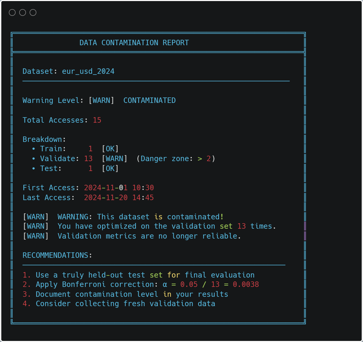
Cache Safety and Data Contamination
The most important feature of the caching system is contamination prevention. Every data access is logged:
@cacheable(time_aware=True)
def load_and_prepare_training_data(...):
    # ... load data ...
    log_data_access(
            dataset_name=f"{symbol}_{bar_type}_{bar_size}".lower(),
            start_date=data.index[0],
            end_date=data.index[-1],
            purpose="train",
            data_shape=data.shape)

    return data
At any time, you can check for contamination:
from ..cache import print_contamination_report


print_contamination_report()
Practical Usage Patterns
Let me show you some common research workflows:
1. Strategy Comparison
strategies = [
        BollingerBandStrategy(window=20, num_std=2.0),
        BollingerBandStrategy(window=20, num_std=2.5),
        BollingerBandStrategy(window=30, num_std=2.0),
]
results = []

for strategy in strategies:
        pipeline = ModelDevelopmentPipeline(
                                symbol="EURUSD",
                                train_start="2023-01-01",
                                train_end="2023-12-31",
                                strategy=strategy,
                                # ... config ...
                )
        model, features, metrics, config = pipeline.run(verbose=False)
        results.append({
                        "strategy": strategy.get_strategy_name(),
                        "cv_score": metrics["cv_results"]["best_score"],
                        "features": len(features), "model": model
                })

comparison = pd.DataFrame(results).sort_values("cv_score", ascending=False)
print(comparison)
Because of caching, comparing strategies is fast—only the model training changes.
2. Feature Engineering Experiments
feature_configs = [
        {"func": calculate_basic_features, "params": {}},
        {"func": calculate_advanced_features, "params": {"lookback": 20}},
        {"func": calculate_advanced_features, "params": {"lookback": 50}},
        ]

for i, feat_config in enumerate(feature_configs):
        pipeline = ModelDevelopmentPipeline(
			# ... same data config ... feature_config=feat_config,
			# ... rest of config ...
			)
        model, features, metrics, _ = pipeline.run()
	print(f"Feature set {i+1}: {metrics['cv_results']['best_score']:.4f}")
3. Walk-Forward Analysis
train_periods = [
	("2022-01-01", "2022-12-31"),
	("2022-07-01", "2023-06-30"),
	("2023-01-01", "2023-12-31"),
	]
models = []

for train_start, train_end in train_periods:
        pipeline = ModelDevelopmentPipeline(
                                symbol="EURUSD",
                                train_start=train_start,
                                train_end=train_end,
                                # ... config ...
                                )
        model, _, metrics, _ = pipeline.run()
        models.append({
                        "period": f"{train_start} to {train_end}",
                        "score": metrics["cv_results"]["best_score"],
                        "model_path": pipeline.file_paths["model"]
                         })
The organized directory structure makes it easy to compare models across time periods.
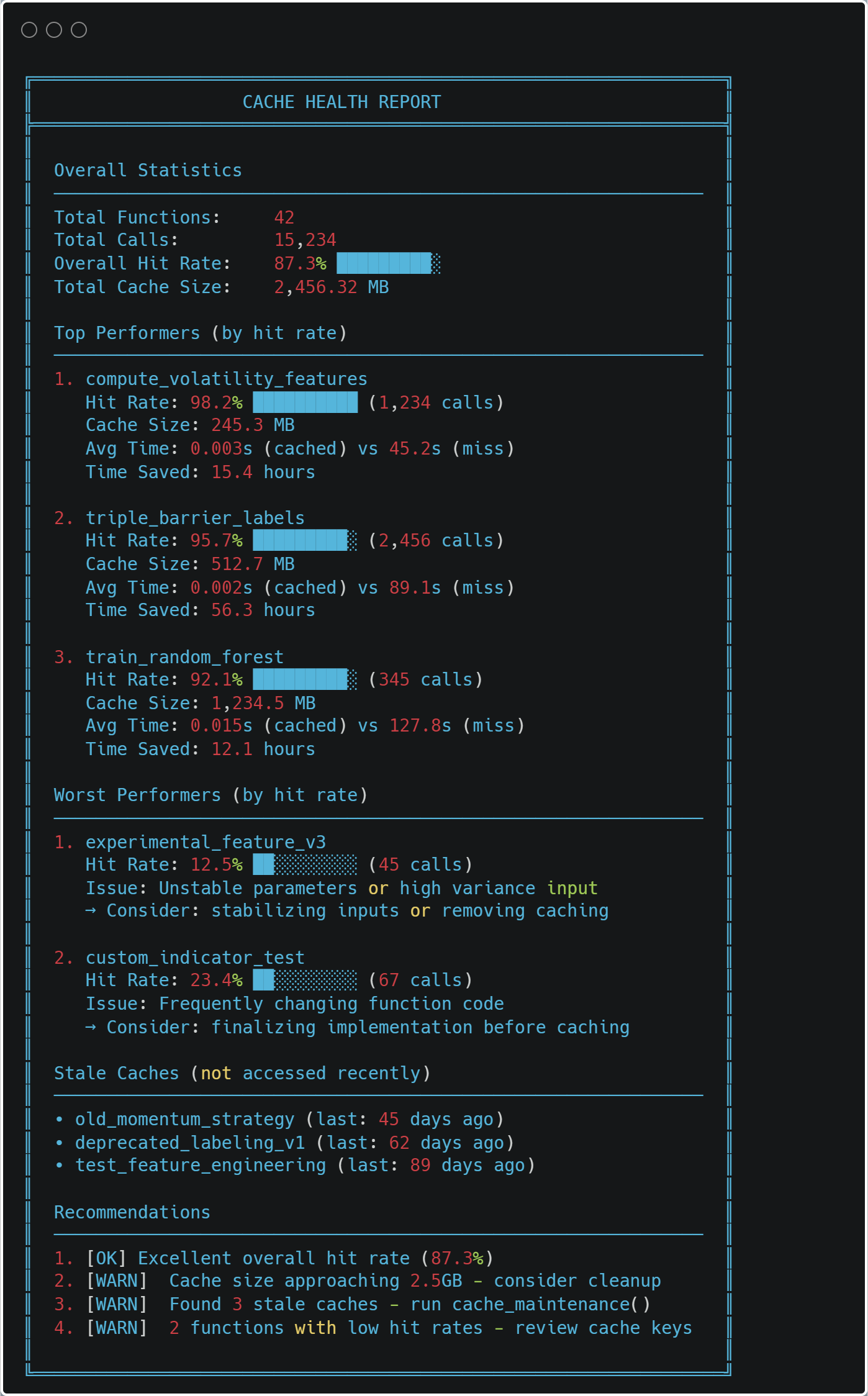
Performance Monitoring
The system tracks its own performance:
from ..cache import print_health_report

print_health_report()
Integration with MQL5
The ONNX export makes deployment straightforward. Here's a minimal MQL5 EA skeleton:
//+------------------------------------------------------------------+
//|                                     BollingerBandStrategy_EA.mq5 |
//+------------------------------------------------------------------+

#property version   "1.00"
#property strict

//--- Include Resources
#include <Trade\Trade.mqh>

//--- Load the ONNX model from resources
#resource "\\Models\\BollingerBandStrategy\\EURUSD\\model.onnx" as uchar model_data[]

//--- Input Parameters
input double   InpLotSize      = 0.01;   // Trade Lot Size
input double   InpThresholdBuy = 0.55;   // Probability to Buy
input double   InpThresholdExit = 0.45;  // Probability to Exit/Sell

//--- Global Variables
long           model_handle    = INVALID_HANDLE;
CTrade         trade;

//+------------------------------------------------------------------+
//| Expert initialization function                                   |
//+------------------------------------------------------------------+
int OnInit()
{
    // Load ONNX model from the resource buffer
    model_handle = OnnxCreateFromBuffer(model_data, ONNX_DEFAULT);

    if(model_handle == INVALID_HANDLE)
    {
        Print("Error: Failed to load ONNX model. Code: ", GetLastError());
        return(INIT_FAILED);
    }

    // Set output shape if necessary (depends on your model export)
    // OnnxSetOutputShape(model_handle, 0, [1, 1]);

    Print("Model loaded successfully. Handle: ", model_handle);
    return(INIT_SUCCEEDED);
}

//+------------------------------------------------------------------+
//| Expert deinitialization function                                 |
//+------------------------------------------------------------------+
void OnDeinit(const int reason)
{
    if(model_handle != INVALID_HANDLE)
    {
        OnnxRelease(model_handle);
        model_handle = INVALID_HANDLE;
    }
}

//+------------------------------------------------------------------+
//| Expert tick function                                             |
//+------------------------------------------------------------------+
void OnTick()
{
    // 1. Prepare Features
    double features[47];
    if(!CalculateFeatures(features)) return;

    // 2. Prepare ONNX Vectors
    vector v_features;
    v_features.Assign(features);
    vector v_output;

    // 3. Run Inference
    if(!OnnxRun(model_handle, ONNX_NO_CONVERSION, v_features, v_output))
    {
        Print("Inference failed. Error: ", GetLastError());
        return;
    }

    // 4. Trade Logic
    double probability = v_output[0];
    CheckTradeLogic(probability);
}

//+------------------------------------------------------------------+
//| Logic for Entry and Exit                                         |
//+------------------------------------------------------------------+
void CheckTradeLogic(double prob)
{
    bool hasPosition = (PositionsTotal() > 0);

    // Buy Logic
    if(prob > InpThresholdBuy && !hasPosition)
    {
        trade.Buy(InpLotSize, _Symbol, SymbolInfoDouble(_Symbol, SYMBOL_ASK), 0, 0, "ONNX Signal");
    }
    // Exit Logic
    else if(prob < InpThresholdExit && hasPosition)
    {
        trade.PositionClose(_Symbol);
    }
}

//+------------------------------------------------------------------+
//| Feature Calculation - MUST MATCH PYTHON PRE-PROCESSING           |
//+------------------------------------------------------------------+
bool CalculateFeatures(double &features[])
{
    ArrayInitialize(features, 0.0);

    // Example: Getting Bollinger Bands data for the current bar
    double bb_upper = iBands(_Symbol, PERIOD_CURRENT, 20, 2.0, 0, PRICE_CLOSE, MODE_UPPER, 0);
    double bb_lower = iBands(_Symbol, PERIOD_CURRENT, 20, 2.0, 0, PRICE_CLOSE, MODE_LOWER, 0);
    double close    = iClose(_Symbol, PERIOD_CURRENT, 0);

    // Fill your 47 features here exactly as your model expects
    // features[0] = (close - bb_lower) / (bb_upper - bb_lower); // Normalized example
    // ...

    return true;
}
The key is ensuring your MQL5 features exactly match your Python features. The training summary's feature list helps with this.
Debugging and Troubleshooting
When something goes wrong, the system provides detailed diagnostics:
Example: Model Performance Drops
# Get all experiments for a symbol
file_manager = ModelFileManager("Models")
models = file_manager.find_models({ "symbol": "EURUSD", "strategy": "BollingerBandStrategy" })

# Compare performance over time
for model_info in models:
        metrics = json.load(open(model_info["file_path"].replace(".joblib", "_metrics.json")))
        print(f"{model_info['date_range']}: {metrics['cv_results']['best_score']:.4f}")
You can quickly identify when performance changed and load the corresponding configuration to see what was different.
Example: Cache Issues
If you suspect cache corruption:
from cache import clear_cache

# Clear specific function cache
clear_cache("load_and_prepare_training_data")

# Or clear everything
clear_cache()
The system will rebuild from scratch, ensuring correctness.
Best Practices
After using this system for months, here are my recommendations:
1. Always Use Descriptive Strategy Names
# Good strategy name
BollingerBandStrategy(window=20, num_std=2.0)
strategy.get_strategy_name() # "BollingerBand_w20_std2.0"

# Better - includes your hypothesis strategy
BollingerBandStrategy(window=20, num_std=2.0, name="BB_MeanReversion_v1")
Your future self will thank you when browsing 50 experiments.
2. Start with Small Parameter Grids
# First iteration - quick feedback
param_grid = {
	"n_estimators": [100, 200],
	"max_depth": [3, 5, 7]
	}

# After you understand the landscape
param_grid = {
	"n_estimators": [100, 200, 300, 500],
	"max_depth": [3, 5, 7, 10, 15],
	"min_samples_split": [2, 5, 10, 20]
	}
Iterate quickly first, then refine.
3. Save Everything
Storage is cheap, reproducibility is priceless:
pipeline.run(
        generate_reports=True, # Always
        save=True, # Always
        export_onnx=True, # If deploying
        verbose=True # Until you're confident
        )
4. Review Reports Before Deployment
Don't deploy based on CV score alone. Check:
- Fold consistency (high variance = unreliable)
- Feature importance (sensible features?)
- Label distribution (balanced?)
- ONNX validation (passed?)
The reports make this easy.
5. Version Your Feature Functions
def calculate_features_v1(data, **params):
        """Initial feature set - baseline."""
        # ... features ...

def calculate_features_v2(data, **params):
        """Added momentum indicators."""
        # ... features ...

feature_config = { "func": calculate_features_v2, # Track version in function name
                   "params": {}
		}
When you improve features, create a new function. The cache will automatically handle versioning.
Conclusion
Building a production-grade research system requires upfront investment, but the payoff is enormous:
- Speed: 10x more experiments in the same time
- Reliability: Reproducible results you can trust
- Insight: Automatic analysis reveals patterns you'd miss
- Deployment: One-button export to MQL5
- Maintenance: Easy to debug, easy to extend
The code we've explored exhibits some of the most critical aspects of a financial ML research methodology. It enforces best practices: proper cross-validation, sample weighting, feature analysis (albeit very limited), and validation. It makes the right way the easy way.
Most importantly, it lets you focus on what matters: developing better trading strategies. The plumbing just works.
Next Steps
To implement this system:
- Start Small: Begin with a single strategy and symbol
- Verify Caching: Run the pipeline twice, confirm speedup
- Check Reports: Review all generated reports
- Validate ONNX: Ensure predictions match perfectly
- Deploy Carefully: Start with paper trading
- Iterate: Use the system to run systematic experiments
The full code is available in the accompanying files. Start with model_development.py in the folder "production", and work through the example notebook.
Remember: trading is hard enough without fighting your research tools. Build systems that help you win.
File Reference Guide
| File | Primary Purpose | Key Classes/Functions | Dependencies | When to Use |
|---|---|---|---|---|
| __init__.py | Module exports | complete_export_workflow() export_model_to_onnx() extract_onnx_metadata() validate_onnx_predictions() | model_export.py | Exposes the ONNX export functionality at the package level |
| dual_model_development.py | Bid/Ask-aware separate long/short models | BidAskLongShortPipeline train_bidask_longshort_models() | model_development.py, strategy classes | When you need separate models for long and short positions using realistic execution prices (long → ask, short → bid) |
| model_development.py | Core production pipeline | ModelDevelopmentPipeline TickDataLoader load_and_prepare_training_data() generate_events_triple_barrier() train_model_with_cv() | feature_engine, sklearn, numba, cache system | The main pipeline for training and evaluating any single model with full reproducibility |
| model_export.py | ONNX conversion and validation | export_model_to_onnx() validate_onnx_predictions() complete_export_workflow() | skl2onnx, onnxruntime | Final step before MQL5 deployment - ensures production model matches Python exactly |
| utils.py | File management and organization | ConfigPathGenerator ModelFileManager find_models() load_artifacts() | hashlib, json, pickle, pathlib | Managing the model directory structure, saving/loading artifacts, and finding past experiments |
File Relationships:
- __init__.py → model_export.py (exposes export functions)
- dual_model_development.py → model_development.py (extends the base pipeline)
- model_development.py → utils.py (uses file management)
- model_export.py → Standalone (can work independently)
- All files → Cache system (for performance)
Key Integration Points:
- dual_model_development.py creates two ModelDevelopmentPipeline instances (long/short)
- ModelFileManager in utils.py is used by ModelDevelopmentPipeline for organized storage
- export_model_to_onnx() is called from ModelDevelopmentPipeline when export_onnx=True
Warning: All rights to these materials are reserved by MetaQuotes Ltd. Copying or reprinting of these materials in whole or in part is prohibited.
This article was written by a user of the site and reflects their personal views. MetaQuotes Ltd is not responsible for the accuracy of the information presented, nor for any consequences resulting from the use of the solutions, strategies or recommendations described.

- Free trading apps
- Over 8,000 signals for copying
- Economic news for exploring financial markets
You agree to website policy and terms of use