Neuroboids Optimization Algorithm (NOA)

Contents

1. Introduction
2. Implementation of the algorithm
3. Test results

Introduction

While researching optimization algorithms, I was always drawn to the idea of creating the simplest, yet most efficient solutions possible. Observing how nature solves complex problems through the interaction of simple organisms, I developed a new optimization algorithm - the Neuroboids Optimization Algorithm (NOA).

The algorithm is based on the concept of minimalistic neural agents – neuroboids. Each neuroboid is a simple neural network with two layers of neurons, which is trained using the Adam algorithm. The uniqueness of this approach lies in the fact that, despite the extreme simplicity of individual agents, their collective behavior must effectively explore the solution space of complex optimization problems.

The inspiration for NOA came from the processes of self-organization in natural systems, where simple units, following basic rules, form complex adaptive structures. In this article, I present the theoretical justification of the algorithm, its mathematical model, and the results of an experimental study of its efficiency on standard optimization test functions.

Implementation of the algorithm

Imagine that you are walking in the garden after the rain. Earthworms are everywhere - simple creatures with a primitive nervous system. They do not have the ability to "think" in our sense, but somehow they find their way through difficult terrain, avoid danger, find food and partners. Their tiny brains contain only a few thousand neurons, yet they have existed for millions of years. This is how the idea of neuroboids was born.

What if we combined the simplicity of a worm with the power of collective intelligence? In nature, simple organisms achieve incredible results when they work together — ants build complex colonies, bees solve optimization problems when collecting nectar, and flocks of birds form complex dynamic structures without centralized control.

My neuroboids are like these earthworms. Each one has its own small neural network - not some massive architecture with millions of parameters, but just a few neurons at the input and output. They do not know the entire search space, they only see their local environment. When one worm finds a fertile patch of soil rich in nutrients, others gradually gravitate towards that spot. But they do not just follow blindly – each one maintains their own individuality, their own movement strategy. The neuroboids do not need to know all the math behind optimization. They learn on their own, through trial and error. When one of them finds a good solution, the others do not just copy its coordinates, but learn to understand why this solution is good and how to get there on their own.

Remember sunsets at sea? The sun is reflected in millions of glares on the waves, and each glare is its own little story of the interaction of light with water. The same is true for my neuroboids - each one reflects a part of the solution, and together they create a complete picture. From a distance, their movement may appear chaotic. But within this apparent chaos, order is born – a self-organizing system for finding optimal solutions.

The neuroboids also have no central commander. Instead, each uses its own small neural network to decide whether to follow the best known solution or explore new territory, copy a neighbor's successful strategy or risk creating its own. 

In the world obsessed with complexity and scale, neuroboids are a reminder that the greatest systems are often built from the simplest elements. Just as grains of sand form beaches and mountains, and droplets form oceans, so too do my little digital worms, each with its own tiny neural network, work together to solve problems that giant, monolithic algorithms fail to solve.

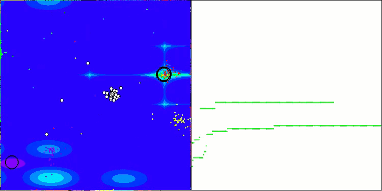
Figure 1. NOA algorithm operation

Figure 1 shows the main components and operating principle of the NOA algorithm. The search space is the domain in which neuroboids (blue circles) search for the optimal solution. Neuroboids are optimization agents, each with its own neural network. The best solution is the current best solution found (the golden circle) toward which the neuroboids strive. The neural network architecture is as follows: each neuroboid uses its own neural network to determine the direction of movement. The algorithm cyclical process consists of the following stages: initialization — random placement of neuroboids; neural network training — learning based on the best solution found; neuroboids move under the control of the trained neural networks; the best solution is updated if a better one is found. The dotted lines show the directions of movement of the neuroboids, which are determined by the outputs of their neural networks and striving for the best solution with an element of randomness.

The term "neuroboid" combines the concepts of a neural network and a boid (an artificial "bird" in models of collective behavior). Each neuroboid agent is a combination of a position in the solution space
and a personal neural network that determines the movement strategy.

Unlike traditional metaheuristic algorithms (such as genetic algorithms or swarm methods), where the behavior of agents is determined by fixed rules, in NOA: each neuronode has its own neural network, which is trained during the optimization; neural networks gradually learn to determine the most promising search directions, and training occurs based on the best solution found (target vector). It turns out that the optimization algorithm includes two search strategies: the first is NOA itself, and the second is ADAM built into the neural network. The backpropagation mechanism allows ADAM to be used in the context of the NOA algorithm as an independent tool for adjusting the neural network weights of each neuron. Consequently, the total number of weights of all neuron bodies can be much larger than the problem dimension — there is no need to optimize the neural network weights of the entire population; this happens naturally and automatically.

The behavior of neuroboids has certain parallels with: social learning in nature (observation of successful individuals), neuroplasticity (the ability of the nervous system to adapt to changing conditions) and collective intelligence (emergent optimization through the interaction of many simple agents).

The main technical features of the NOA algorithm can be identified:

• forward and backward propagation of errors within the optimization,
• distributed training of multiple neural networks, each of which forms its own strategy,
• adaptive behavior adjustment based on the current search state,
• using activation functions of neural networks to create non-linear search dynamics.

This combination makes NOA an interesting hybrid approach that combines machine learning and optimization paradigms. Instead of using neural networks to approximate the objective function (as in surrogate models), NOA uses them to indirectly guide the search itself, creating a kind of "meta-learning" for solving optimization problems.

Now we can write the pseudocode for the NOA algorithm:

Initialization:

1. Create a population of N neural networks (neuroboids)
2. Each neural network has a structure with a number of inputs and outputs equal to the dimension of the optimization problem
3. Set the parameters:
   • popSize (population size)
   • actFunc (neuron activation function)
   • dispScale (displacement scale)
   • eliteProb (probability of copying elite coordinates)

Algorithm:

1. If this is the first iteration (revision = false):
   • For each neuroboid in the population:
     • Randomly initialize coordinates in the search space
     • Convert coordinates to acceptable discrete values
   • Set revision = true and terminate the current iteration
2. For subsequent iterations:
   • For most neuroboids (all but the last 5):
     • For each coordinate:
       • With the eliteProb probability, replace the coordinate value with the value from the best solution found (cB)
   • For each neuroboid in the population:
     • Scale the best solution found (cB) and the current position of the neuroboid to the range [-1, 1]
     • Perform forward propagation through the neural network of the current neuroboid
     • Calculate the error between the target value (scaled by cB) and the output of the neural network
     • Perform backpropagation to train the neural network
     • Update the coordinates of the neuroboid by shifting them in the direction determined by the output of the neural network
     • Convert coordinates to acceptable discrete values
3. Rating and update:
   • For each neuroboid in the population:
     • Calculate the value of the objective function for the current coordinates
     • If the value is better than the best found (fB):
       • Update best found value (fB)
       • Save current coordinates as best (cB)

Let's start writing the algorithm code. Define the C_AO_NOA class, which is derived from the C_AO class. This means that it inherits the properties and methods of C_AO and also adds its own. Main elements of the class:

~C_AO_NOA () destructor: removes dynamically allocated activation function objects for each element of the "nn" array - the individual neural network of neuroboids. This helps prevent memory leaks.

C_AO_NOA () constructor:

• Initializes the optimization algorithm parameters.
• Sets initial values for the parameters: popSize - population size, actFunc - neuron activation function, dispScale - movement scale, probability of copying elite coordinates.
• Reserve the "params" array to store parameters.

SetParams () method: sets parameters based on the values stored in the "params" array.

Init () method: defined to initialize the class with the value ranges of rangeMinP, rangeMaxP and rangeStepP, as well as the epochsP number of epochs. 

Moving () and Revision (): these methods serve to move individuals in the population and perform the evaluation and updating of decisions.

nn array: an array of instances of the neural network class of each neuroboid.

Closed methods: ScaleInp () and ScaleOut () - methods for scaling input and output data, respectively.

//——————————————————————————————————————————————————————————————————————————————
class C_AO_NOA : public C_AO
{
  public: //--------------------------------------------------------------------
  ~C_AO_NOA ()
  {
    for (int i = 0; i < ArraySize (nn); i++) if (CheckPointer (nn [i].actFunc)) delete nn [i].actFunc;
  }
  C_AO_NOA ()
  {
    ao_name = "NOA";
    ao_desc = "Neuroboids Optimization Algorithm (joo)";
    ao_link = "https://www.mql5.com/en/articles/16992";

    popSize   = 50;   // population size
    actFunc   = 0;    // neuron activation function
    dispScale = 0.01; // scale of movements
    eliteProb = 0.1;  // probability of copying elite coordinates

    ArrayResize (params, 4);
    params [0].name = "popSize";   params [0].val  = popSize;
    params [1].name = "actFunc";   params [1].val  = actFunc;
    params [2].name = "dispScale"; params [2].val  = dispScale;
    params [3].name = "eliteProb"; params [3].val  = eliteProb;
  }

  void SetParams ()
  {
    popSize   = (int)params [0].val;
    actFunc   = (int)params [1].val;
    dispScale = params      [2].val;
    eliteProb = params      [3].val;
  }

  bool Init (const double &rangeMinP  [],  // minimum values
             const double &rangeMaxP  [],  // maximum values
             const double &rangeStepP [],  // step change
             const int     epochsP = 0);   // number of epochs

  void Moving   ();
  void Revision ();

  //----------------------------------------------------------------------------
  int    actFunc;   // neuron activation function
  double dispScale; // scale of movements
  double eliteProb; // probability of copying elite coordinates

  private: //-------------------------------------------------------------------
  C_MLPa nn [];

  void ScaleInp (double &inp [], double &out []);
  void ScaleOut (double &inp [], double &out []);
};
//——————————————————————————————————————————————————————————————————————————————

The Init method is intended to initialize an instance of the C_AO_NOA class. It takes a number of parameters that specify the range of values and the number of epochs, and performs the necessary operations to tune the algorithm.

Method signature: indicates that the initialization was successful. Parameters:

• MinP [] - minimum values for parameters.
• MaxP [] - maximum values for parameters.
• StepP [] - step for changing parameters.
• epochsP - number of epochs.

Standard initialization: the first line of the method calls the StandardInit function with the passed ranges.

Setting up neural network configuration:

• The nnConf array is created, which contains the sizes of the input and output layers of the neural network.
• The ArrayResize is called to resize the nnConf array to 2 (input and output layer).
• Both array elements are initialized with the "coords" value, which corresponds to the dimensions of the input data.

E_Act enumeration declaration: an enumeration is created that defines different neuron activation functions (eActTanh, eActAlgSigm, eActRatSigm etc.).

Backing up the neuron array: resizes the "nn" array (the array of neurons) to popSize, which was previously set in the constructor.

Initialization of neurons:

• The cnt variable is initialized from zero and is used to pass a unique random seed to initialize each neuron, ensuring that the weights in each neural network are uniquely initialized.
• Each neuron is initialized in the "for" loop. The nn[i].Init() method is called with the nnConf configuration, the actFunc activation function, and a seed based on the current cnt value and the number of milliseconds elapsed since the system started.
• The cnt value is incremented with each loop iteration, allowing for unique seeds to be generated for each neuron initialization.

Return the result: if all operations are successful, the method returns "true", the initialization was successful.

The Init method of the С_AO_NOA class is key to setting up the optimization algorithm, providing initialization of the neural network and associated parameters. 

//——————————————————————————————————————————————————————————————————————————————
bool C_AO_NOA::Init (const double &rangeMinP  [], // minimum values
                     const double &rangeMaxP  [], // maximum values
                     const double &rangeStepP [], // step change
                     const int     epochsP = 0)   // number of epochs
{
  if (!StandardInit (rangeMinP, rangeMaxP, rangeStepP)) return false;

  //----------------------------------------------------------------------------
  int nnConf [];
  ArrayResize (nnConf, 2);
  nnConf [0] = coords;
  nnConf [1] = coords;

  enum E_Act
  {
    eActTanh,      //0
    eActAlgSigm,   //1
    eActRatSigm,   //2

    eActSoftPlus,  //3
    eActBentIdent, //4
    eActSiLU,      //5

    eActACON,      //6
    eActSERF,      //7
    eActSnake      //8
  };

  ArrayResize (nn, popSize);
  int cnt = 0;
  for (int i = 0; i < popSize; i++)
  {
    nn [i].Init (nnConf, actFunc, (int)GetTickCount64 () + cnt);
    cnt++;
  }

  return true;
}
//——————————————————————————————————————————————————————————————————————————————

The Moving() method implements moving individuals in a population within the framework of a neuron-like optimization algorithm. Let's break it down step by step:

Initialization of initial values: if 'revision' is 'false', the method performs the first initialization. For each element in the popSize population and for each coords dimension, the method sets the initial values in the a[i].c[c] array representing the search agents:

• u.RNDfromCI () generates a random value in the rangeMin[c] and rangeMax[c] range.
• u.SeInDiSp() is a function that uses a step change to adjust the value of a [i].c [c] within a valid range.
• After initialization is complete, 'revision' is set to 'true' and control returns from the method. 

Updating coordinates: The coordinates of individuals are updated based on the probability of eliteness. For the first popSize - 5 elements of the population, a random check is performed, and if the random number is less than eliteProb, the a [i].c [c] coordinates are set equal to the coordinates of the "cB [c]" elite.

Handling neural network data: arrays for input and output data, target values and errors are created and prepared to the 'coords' size. For each element of the population:

• ScaleInp () scales the cB target coordinates and stores them in targVal.
• ScaleInp () - scales the current coordinate from the population and stores it in inpData.
• nn [i].ForwProp () performs forward propagation on the neural network to produce output.
• The error (the difference between the target and the obtained value) is calculated for each coordinate.
• nn [i].BackProp (err) performs backpropagation of the error to adjust the weights.
• The a [i].c [c] coordinates are updated taking into account the output of the neural network, scaling, and a random sample element.
• At the end, the value of a[i].c[c] is normalized by the u.SeInDiSp function.

Thus, the Moving() method is responsible for moving individuals in the model, initializing them at the beginning and updating their positions based on the outputs of neural networks and probabilistic choices. 

//——————————————————————————————————————————————————————————————————————————————
void C_AO_NOA::Moving ()
{
  //----------------------------------------------------------------------------
  if (!revision)
  {
    // Initialize the initial values of anchors in all parallel universes
    for (int i = 0; i < popSize; i++)
    {
      for (int c = 0; c < coords; c++)
      {
        a [i].c [c] = u.RNDfromCI (rangeMin [c], rangeMax [c]);
        a [i].c [c] = u.SeInDiSp  (a [i].c [c], rangeMin [c], rangeMax [c], rangeStep [c]);
      }
    }

    revision = true;
    return;
  }

  //----------------------------------------------------------------------------
  double rnd  = 0.0;
  double val  = 0.0;
  int    pair = 0.0;

  for (int i = 0; i < popSize - 5; i++)
  {
    for (int c = 0; c < coords; c++)
    {
      if (u.RNDprobab () < eliteProb)
      {
        a [i].c [c] = cB [c];
      }
    }
  }

  double inpData []; ArrayResize (inpData, coords);
  double outData []; ArrayResize (outData, coords);
  double targVal []; ArrayResize (targVal, coords);
  double err     []; ArrayResize (err,     coords);

  for (int i = 0; i < popSize; i++)
  {
    ScaleInp (cB,      targVal);
    ScaleInp (a [i].c, inpData);

    nn [i].ForwProp (inpData, outData);

    for (int c = 0; c < coords; c++) err [c] = targVal [c] - outData [c];

    nn [i].BackProp (err);

    for (int c = 0; c < coords; c++)
    {
      a [i].c [c] += outData [c] * (rangeMax [c] - rangeMin [c]) * dispScale * u.RNDprobab ();
      a [i].c [c] = u.SeInDiSp  (a [i].c [c], rangeMin [c], rangeMax [c], rangeStep [c]);
    }
  }
}
//——————————————————————————————————————————————————————————————————————————————

Let's next examine the Revision method, which evaluates and updates the current "best" solution in the population. It compares the objective function values for each individual with the current "best" value and updates it if it finds a better one. Thus, the method ensures that the current best solution is maintained in the population. 

//——————————————————————————————————————————————————————————————————————————————
void C_AO_NOA::Revision ()
{
  for (int i = 0; i < popSize; i++)
  {
    if (a [i].f > fB)
    {
      fB = a [i].f;
      ArrayCopy (cB, a [i].c);
    }
  }
}
//——————————————————————————————————————————————————————————————————————————————

The ScaleInp method is responsible for scaling the input data from the range specified by rangeMin and rangeMax to the interval from -1 to 1. Each value of inp[c] is scaled using the u.Scale function, which performs a linear scaling to bring it into the range from -1 to 1. The ScaleInp method prepares data for further calculations, ensuring its normalization to the desired range.

//——————————————————————————————————————————————————————————————————————————————
void C_AO_NOA::ScaleInp (double &inp [], double &out [])
{
  for (int c = 0; c < coords; c++) out [c] = u.Scale (inp [c], rangeMin [c], rangeMax [c], -1, 1);
}
//——————————————————————————————————————————————————————————————————————————————

The ScaleOut method works similarly to ScaleInp, which performs inverse scaling from the range from -1 to 1 into the rangeMin and rangeMax interval.

//——————————————————————————————————————————————————————————————————————————————
void C_AO_NOA::ScaleOut (double &inp [], double &out [])
{
  for (int c = 0; c < coords; c++) out [c] = u.Scale (inp [c], -1, 1, rangeMin [c], rangeMax [c]);
}
//——————————————————————————————————————————————————————————————————————————————

Test results

The algorithm shows interesting results on functions with small and moderate dimensions. When the problem size increases to 1000 variables, the computation time becomes unacceptably large, as a result of which these tests are not presented. Performance reaches about 45% (for 6 tests out of 9) of the optimal value according to the tests.

NOA|Neuroboids Optimization Algorithm (joo)|50.0|0.0|0.01|0.1|
=============================
5 Hilly's; Func runs: 10000; result: 0.7013521128826248
25 Hilly's; Func runs: 10000; result: 0.40128968110640306
=============================
5 Forest's; Func runs: 10000; result: 0.6222984295200933
25 Forest's; Func runs: 10000; result: 0.30830340651626337
=============================
5 Megacity's; Func runs: 10000; result: 0.4523076923076924
25 Megacity's; Func runs: 10000; result: 0.20892307692307693
=============================
All score: 2.69447 (44.91%)

I would like to say a few words about the visualization of the NOA algorithm. As you can see, the algorithm forms interesting fan-shaped structures. In essence, these structures are a visualization of the results of the neural networks in neuroboids. 

NOA on the Hilly test function

NOA on the Forest test function

NOA on the Megacity test function

After the tests the NOA algorithm is placed in a separate line (it does not have a serial number), since no testing results were obtained on high-dimensional functions. The tables below are presented for comparative analysis of results with other algorithms participating in the rating table.

#	AO	Description	Hilly			Hilly final	Forest			Forest final	Megacity (discrete)			Megacity final	Final result	% of MAX
			10 p (5 F)	50 p (25 F)	1000 p (500 F)		10 p (5 F)	50 p (25 F)	1000 p (500 F)		10 p (5 F)	50 p (25 F)	1000 p (500 F)
1	ANS	across neighbourhood search	0.94948	0.84776	0.43857	2.23581	1.00000	0.92334	0.39988	2.32323	0.70923	0.63477	0.23091	1.57491	6.134	68.15
2	CLA	code lock algorithm (joo)	0.95345	0.87107	0.37590	2.20042	0.98942	0.91709	0.31642	2.22294	0.79692	0.69385	0.19303	1.68380	6.107	67.86
3	AMOm	animal migration ptimization M	0.90358	0.84317	0.46284	2.20959	0.99001	0.92436	0.46598	2.38034	0.56769	0.59132	0.23773	1.39675	5.987	66.52
4	(P+O)ES	(P+O) evolution strategies	0.92256	0.88101	0.40021	2.20379	0.97750	0.87490	0.31945	2.17185	0.67385	0.62985	0.18634	1.49003	5.866	65.17
5	CTA	comet tail algorithm (joo)	0.95346	0.86319	0.27770	2.09435	0.99794	0.85740	0.33949	2.19484	0.88769	0.56431	0.10512	1.55712	5.846	64.96
6	TETA	time evolution travel algorithm (joo)	0.91362	0.82349	0.31990	2.05701	0.97096	0.89532	0.29324	2.15952	0.73462	0.68569	0.16021	1.58052	5.797	64.41
7	SDSm	stochastic diffusion search M	0.93066	0.85445	0.39476	2.17988	0.99983	0.89244	0.19619	2.08846	0.72333	0.61100	0.10670	1.44103	5.709	63.44
8	BOAm	billiards optimization algorithm M	0.95757	0.82599	0.25235	2.03590	1.00000	0.90036	0.30502	2.20538	0.73538	0.52523	0.09563	1.35625	5.598	62.19
9	AAm	archery algorithm M	0.91744	0.70876	0.42160	2.04780	0.92527	0.75802	0.35328	2.03657	0.67385	0.55200	0.23738	1.46323	5.548	61.64
10	ESG	evolution of social groups (joo)	0.99906	0.79654	0.35056	2.14616	1.00000	0.82863	0.13102	1.95965	0.82333	0.55300	0.04725	1.42358	5.529	61.44
11	SIA	simulated isotropic annealing (joo)	0.95784	0.84264	0.41465	2.21513	0.98239	0.79586	0.20507	1.98332	0.68667	0.49300	0.09053	1.27020	5.469	60.76
12	ACS	artificial cooperative search	0.75547	0.74744	0.30407	1.80698	1.00000	0.88861	0.22413	2.11274	0.69077	0.48185	0.13322	1.30583	5.226	58.06
13	DA	dialectical algorithm	0.86183	0.70033	0.33724	1.89940	0.98163	0.72772	0.28718	1.99653	0.70308	0.45292	0.16367	1.31967	5.216	57.95
14	BHAm	black hole algorithm M	0.75236	0.76675	0.34583	1.86493	0.93593	0.80152	0.27177	2.00923	0.65077	0.51646	0.15472	1.32195	5.196	57.73
15	ASO	anarchy society optimization	0.84872	0.74646	0.31465	1.90983	0.96148	0.79150	0.23803	1.99101	0.57077	0.54062	0.16614	1.27752	5.178	57.54
16	RFO	royal flush optimization (joo)	0.83361	0.73742	0.34629	1.91733	0.89424	0.73824	0.24098	1.87346	0.63154	0.50292	0.16421	1.29867	5.089	56.55
17	AOSm	atomic orbital search M	0.80232	0.70449	0.31021	1.81702	0.85660	0.69451	0.21996	1.77107	0.74615	0.52862	0.14358	1.41835	5.006	55.63
18	TSEA	turtle shell evolution algorithm (joo)	0.96798	0.64480	0.29672	1.90949	0.99449	0.61981	0.22708	1.84139	0.69077	0.42646	0.13598	1.25322	5.004	55.60
19	DE	differential evolution	0.95044	0.61674	0.30308	1.87026	0.95317	0.78896	0.16652	1.90865	0.78667	0.36033	0.02953	1.17653	4.955	55.06
20	SRA	successful restaurateur algorithm (joo)	0.96883	0.63455	0.29217	1.89555	0.94637	0.55506	0.19124	1.69267	0.74923	0.44031	0.12526	1.31480	4.903	54.48
21	CRO	chemical reaction optimization	0.94629	0.66112	0.29853	1.90593	0.87906	0.58422	0.21146	1.67473	0.75846	0.42646	0.12686	1.31178	4.892	54.36
22	BIO	blood inheritance optimization (joo)	0.81568	0.65336	0.30877	1.77781	0.89937	0.65319	0.21760	1.77016	0.67846	0.47631	0.13902	1.29378	4.842	53.80
23	BSA	bird swarm algorithm	0.89306	0.64900	0.26250	1.80455	0.92420	0.71121	0.24939	1.88479	0.69385	0.32615	0.10012	1.12012	4.809	53.44
24	HS	harmony search	0.86509	0.68782	0.32527	1.87818	0.99999	0.68002	0.09590	1.77592	0.62000	0.42267	0.05458	1.09725	4.751	52.79
25	SSG	saplings sowing and growing	0.77839	0.64925	0.39543	1.82308	0.85973	0.62467	0.17429	1.65869	0.64667	0.44133	0.10598	1.19398	4.676	51.95
26	BCOm	bacterial chemotaxis optimization M	0.75953	0.62268	0.31483	1.69704	0.89378	0.61339	0.22542	1.73259	0.65385	0.42092	0.14435	1.21912	4.649	51.65
27	ABO	african buffalo optimization	0.83337	0.62247	0.29964	1.75548	0.92170	0.58618	0.19723	1.70511	0.61000	0.43154	0.13225	1.17378	4.634	51.49
28	(PO)ES	(PO) evolution strategies	0.79025	0.62647	0.42935	1.84606	0.87616	0.60943	0.19591	1.68151	0.59000	0.37933	0.11322	1.08255	4.610	51.22
29	TSm	tabu search M	0.87795	0.61431	0.29104	1.78330	0.92885	0.51844	0.19054	1.63783	0.61077	0.38215	0.12157	1.11449	4.536	50.40
30	BSO	brain storm optimization	0.93736	0.57616	0.29688	1.81041	0.93131	0.55866	0.23537	1.72534	0.55231	0.29077	0.11914	0.96222	4.498	49.98
31	WOAm	wale optimization algorithm M	0.84521	0.56298	0.26263	1.67081	0.93100	0.52278	0.16365	1.61743	0.66308	0.41138	0.11357	1.18803	4.476	49.74
32	AEFA	artificial electric field algorithm	0.87700	0.61753	0.25235	1.74688	0.92729	0.72698	0.18064	1.83490	0.66615	0.11631	0.09508	0.87754	4.459	49.55
33	AEO	artificial ecosystem-based optimization algorithm	0.91380	0.46713	0.26470	1.64563	0.90223	0.43705	0.21400	1.55327	0.66154	0.30800	0.28563	1.25517	4.454	49.49
34	ACOm	ant colony optimization M	0.88190	0.66127	0.30377	1.84693	0.85873	0.58680	0.15051	1.59604	0.59667	0.37333	0.02472	0.99472	4.438	49.31
35	BFO-GA	bacterial foraging optimization - ga	0.89150	0.55111	0.31529	1.75790	0.96982	0.39612	0.06305	1.42899	0.72667	0.27500	0.03525	1.03692	4.224	46.93
36	SOA	simple optimization algorithm	0.91520	0.46976	0.27089	1.65585	0.89675	0.37401	0.16984	1.44060	0.69538	0.28031	0.10852	1.08422	4.181	46.45
37	ABHA	artificial bee hive algorithm	0.84131	0.54227	0.26304	1.64663	0.87858	0.47779	0.17181	1.52818	0.50923	0.33877	0.10397	0.95197	4.127	45.85
38	ACMO	atmospheric cloud model optimization	0.90321	0.48546	0.30403	1.69270	0.80268	0.37857	0.19178	1.37303	0.62308	0.24400	0.10795	0.97503	4.041	44.90
39	ADAMm	adaptive moment estimation M	0.88635	0.44766	0.26613	1.60014	0.84497	0.38493	0.16889	1.39880	0.66154	0.27046	0.10594	1.03794	4.037	44.85
40	CGO	chaos game optimization	0.57256	0.37158	0.32018	1.26432	0.61176	0.61931	0.62161	1.85267	0.37538	0.21923	0.19028	0.78490	3.902	43.35
41	ATAm	artificial tribe algorithm M	0.71771	0.55304	0.25235	1.52310	0.82491	0.55904	0.20473	1.58867	0.44000	0.18615	0.09411	0.72026	3.832	42.58
42	ASHA	artificial showering algorithm	0.89686	0.40433	0.25617	1.55737	0.80360	0.35526	0.19160	1.35046	0.47692	0.18123	0.09774	0.75589	3.664	40.71
43	ASBO	adaptive social behavior optimization	0.76331	0.49253	0.32619	1.58202	0.79546	0.40035	0.26097	1.45677	0.26462	0.17169	0.18200	0.61831	3.657	40.63
44	MEC	mind evolutionary computation	0.69533	0.53376	0.32661	1.55569	0.72464	0.33036	0.07198	1.12698	0.52500	0.22000	0.04198	0.78698	3.470	38.55
45	CSA	circle search algorithm	0.66560	0.45317	0.29126	1.41003	0.68797	0.41397	0.20525	1.30719	0.37538	0.23631	0.10646	0.71815	3.435	38.17
	NOA	neuroboids optimization algorithm (joo)	0.70135	0.40129	0.00000	1.10264	0.62230	0.30830	0.00000	0.93060	0.45231	0.20892	0.00000	0.66123	2.694	29.94
	RW	random walk	0.48754	0.32159	0.25781	1.06694	0.37554	0.21944	0.15877	0.75375	0.27969	0.14917	0.09847	0.52734	2.348	26.09

 

Summary

In creating NOA, I aimed to combine two worlds: neural networks and optimization algorithms. The result was both predictable and unexpected.

The main thing that inspires me about this algorithm is its biological plausibility. We often try to create complex models while nature has been demonstrating efficient solutions for millions of years through the collective intelligence of simple organisms. Neuroboids are an attempt to embody this natural wisdom in algorithmic form.

Testing on various functions showed promising results. About 45% efficiency is a decent start for a conceptually new approach. I see that the algorithm performs well in tasks of medium complexity. However, there are also significant limitations. Scalability issues become critical when the problem size is high. At 1000 variables, the computational load becomes impractical due to the need to train multiple neural networks, a process that is itself resource intensive.

What particularly appeals to me about NOA is its ability to self-learn search strategies. Unlike conventional metaheuristics with fixed rules, neuroboids adapt their behavior through learning.

The variability in results between runs that I observed is twofold. On the one hand, it is a lack of predictability. On the other hand, it is a sign of diversity in exploration strategies, which can be an advantage in complex optimization landscapes.

I see several directions for the development of the NOA algorithm:

1. Optimizing neural network architecture to reduce computational load
2. Implementation of knowledge transfer mechanisms between neuroboids

Ultimately, NOA is not just another optimization method. This is a step toward understanding how simple systems can generate complex behavior. This is an exploration of the boundary between machine learning and metaheuristic optimization, between individual and collective intelligence.

I believe this approach has a future not only in function optimization, but also in broader areas – from modeling adaptive behavior to finding fundamentally new artificial intelligence architectures. In the world where complexity is becoming the norm, sometimes simplicity, when properly organized, can yield unexpectedly interesting solutions.

Overall, the NOA algorithm should not be seen as a complete solution to optimization problems, but rather as a basic platform and starting point for many areas of research and the creation of promising solutions in the field of optimization in general and machine learning in particular.

Figure 2. Color gradation of algorithms according to the corresponding tests

Figure 3. Histogram of algorithm testing results (scale from 0 to 100, the higher the better, where 100 is the maximum possible theoretical result, in the archive there is a script for calculating the rating table)

NOA pros and cons:

Pros:

1. Simple implementation.
   
2. Interesting results.

Cons:

1. Due to the long execution time, results for multidimensional spaces were not obtained.
   

The article is accompanied by an archive with the current versions of the algorithm codes. The author of the article is not responsible for the absolute accuracy in the description of canonical algorithms. Changes have been made to many of them to improve search capabilities. The conclusions and judgments presented in the articles are based on the results of the experiments.

• github: https://github.com/JQSakaJoo/Population-optimization-algorithms-MQL5

Programs used in the article

#	Name	Type	Description
1	#C_AO.mqh	Include	Parent class of population optimization algorithms
2	#C_AO_enum.mqh	Include	Enumeration of population optimization algorithms
3	MLPa.mqh	Include	MLP neural network with ADAM
4	TestFunctions.mqh	Include	Library of test functions
5	TestStandFunctions.mqh	Include	Test stand function library
6	Utilities.mqh	Include	Library of auxiliary functions
7	CalculationTestResults.mqh	Include	Script for calculating results in the comparison table
8	Testing AOs.mq5	Script	The unified test stand for all population optimization algorithms
9	Simple use of population optimization algorithms.mq5	Script	A simple example of using population optimization algorithms without visualization
10	Test_AO_NOA.mq5	Script	NOA test stand