Population optimization algorithms: Micro Artificial immune system (Micro-AIS)

Contents

1. Introduction
2. Algorithm
3. Test results

1. Introduction

The immune system is an amazing mechanism that plays an important role in protecting our body from external threats. Like an invisible shield, it fights bacteria, viruses and fungi, keeping our body healthy. But what if we could use this powerful mechanism to solve complex optimization and learning problems? This is exactly the approach used in the Artificial Immune System (AIS) optimization method.

The body's immune system is a complex system of cells, tissues and organs that protects the body from infections, diseases and other external influences. It works by recognizing and destroying foreign substances and microorganisms such as bacteria, viruses, fungi, etc.

The AIS algorithm models these processes using the concepts of antigens (inputs), antibodies (solutions) and killer cells (optimization processes) to optimally solve the problem. Antigens represent the inputs that need to be optimized. Antibodies represent potential solutions to the problem. Killer cells are optimization processes that search for the best solutions to an optimization problem.

Artificial Immune System (AIS) optimization method was proposed in the 1990s. Early research on this method dates back to the mid-1980s, with significant contributions by Farmer, Packard, Perelson (1986) and Bersini and Varela (1990).

Since then, the AIS method has continued to develop and be the subject of ongoing research in the scientific community. Many variations and modifications of this method have been proposed, as well as its application to various optimization and learning problems. The body's immune system also plays an important role in protecting against external influences, such as infections and tumors. It has the ability to recognize and detect anomalies and attack hostile agents, while maintaining the ability to distinguish and store information about them for future use.

Micro-AIS (Micro-Immune Algorithm) is a modification of the immune system (AIS) algorithm that was developed to solve optimization problems. It differs from conventional AIS in that it uses a simpler model of the immune system and simpler immune information processing operations.

The basic idea of Micro-AIS is the creation and evolution of a population of agents that mimic immune cells. Agents move in the solution search space without interacting with each other and without exchanging information about solutions. At the same time, agents can learn and adapt to changing task conditions.

Conventional AIS uses a complex immune system model that includes many types of cells and molecules, such as B cells, T cells, antibodies, cytokines, etc. Micro-AIS uses a simpler model that only includes antibodies. In addition, Micro-AIS uses simpler immune information processing operations, such as mutation and selection.

One of the advantages of Micro-AIS, compared to AIS, is its simplicity and ease of implementation. However, in some cases, a more complex model of the immune system may be more effective for solving complex problems.

Overall, the choice between Micro-AIS and conventional AIS depends on the specific application context. If the optimization problem is relatively simple and a quick solution is required, then Micro-AIS may be a good choice. If the problem is more complex and a more accurate solution is required, then a conventional AIS may be a more suitable choice.

2. Algorithm

Micro-AIS uses the concept of "affinity" to determine suitability, which is a measure of the similarity between an antibody and an antigen. Affinity measures the degree of similarity between an antibody and an antigen. The higher the affinity, the more similar the antibody and antigen are. In Micro-AIS, affinity is used to select the best antibodies to be used to create new antibodies through mutation and crossover. Antibodies with higher affinity are more likely to be selected for the creation of new antibodies.

Affinity can be defined as the distance between the object's feature vector and the classifier's weight vector. The smaller the distance, the more similar the vectors are, and the higher the affinity. In general, affinity can be defined as a function of the distance between two floating point numbers. The distance function can be selected depending on the specific application and requirements of the Micro-AIS algorithm. For example, for optimization problems, distance is usually defined as Euclidean distance, Manhattan distance, or some other type of distance.

However, experiments with Micro-AIS have shown that using affinity is not the most efficient approach in this search strategy, and the fitness function value can be used directly instead.

The original Micro-AIS uses a probabilistic application of mutations to genes. The greater the fitness, the lower the probability of mutation. This approach also had to be abandoned due to inefficiency, which is easy to verify - just add a couple of lines of code.

Micro-AIS pseudo code:

1. Create a population of antibody clones and distribute them randomly across the search space. Antibodies and their clones represent potential solutions to the optimization problem. Clones are created by randomly generating a genotype, which determines the parameter values of the optimization problem.
   
2. Define fitness, which is a measure of the solution quality. The fitness value can be calculated by estimating the objective function for each antibody.
   
3. For each antibody, create clones in an amount corresponding to the rule of decreasing progression: the first antibody (in terms of fitness) creates more clones than the second one, the second one more than the third one, etc. Thus, the number of clones corresponds not to the degree of fitness, but to a strictly defined progression rule. More adapted antibodies create more clones than less adapted ones, always in the same ratio.
   
4. Apply the mutation to the clone genes. For each clone, a genotype mutation occurs, which allows us to create new solutions and explore the parameter space of the optimization problem.
   
5. Determine the fitness of clones.
   
6. After mutation and fitness calculation, the clone population is added to the parent antibody population.
   
7. Sort the population (antibodies + clones) in descending order of fitness in order to subsequently select the best solutions for creating a new population of clones in the next iteration, thereby implementing competition between descendant clones and parent antibodies.
   
8. Repeat from step 2 until the stop criterion is met. The stop criterion can be defined in advance, such as reaching a certain fitness value or reaching the maximum number of iterations.
   

Mutation of genes in clones is the generation of random numbers with a uniform distribution according to the equation:

X' = X + dist * rnd * k * mutation

where:

• X' - new value of the clone gene (coordinates)
• X - parent antibody gene value
• dist - increment to the parent gene
• rnd - random number with uniform distribution in the range [-1.0;1.0]
• k - uniformly decreasing ratio depending on the current epoch
• mutation - mutation ratio, in fact - scale increment factor (external parameter)

The "k" ratio is calculated as follows:

k = (epochs - epochsCNT) / epochs

where:

• epochs - limit value of epochs
• epochsCNT - epoch (iteration) counter

The "dist" increment size is the distance from the maximum value of the optimized parameter to "X" if "rnd" is greater than 0 and from "X" to the minimum value of the optimized parameter if otherwise.

Thus, mutation allows us to randomly change the values of the solution parameters, which ensures exploration of the problem space. The decreasing coefficient "k" allows us to reduce the likelihood of too sudden changes in parameters in later iterations, thereby improving the convergence of the algorithm to the optimal solution and refining the found coordinates.

Let's write a structure that will act as an antibody, S_Agent. The structure contains only two fields:

• c: array of agent coordinates
• f: fitness index
  

The Init method initializes the fields of the structure, changes the size of the "c" array and assigns the initial value "-DBL_MAX" to the "f" field.

//——————————————————————————————————————————————————————————————————————————————
struct S_Agent
{
  void Init (int coords)
  {
    ArrayResize (c, coords);
    f = -DBL_MAX;
  }

  double c []; //coordinates
  double f;    //fitness
};
//——————————————————————————————————————————————————————————————————————————————

Declare the C_AO_Micro_AIS micro-immune system algorithm class, which defines various fields and methods.

Class fields:

• cB: array of best coordinates.
• fB: fitness index for best coordinates.
• a: array of agents of S_Agent type.
• rangeMax: array of maximum search range values.
• rangeMin: array of minimum search range values.
• rangeStep: array of search steps.

The "coords", "popSize", "minClonesNumber", "cloneStep", "mutation" and "epochs" accept the algorithm external parameters.

Class methods:

• Init: initialize the fields of the class with the given values.
• Moving: move agents.
• Revision: perform a revision.

The class also defines "SeInDiSp", "RNDfromCI" and "Sorting" private methods for normalization, random number generation and sorting, respectively.

//——————————————————————————————————————————————————————————————————————————————
class C_AO_Micro_AIS
{
  //----------------------------------------------------------------------------
  public: double  cB [];  //best coordinates
  public: double  fB;     //FF of the best coordinates
  public: S_Agent a  [];  //agent

  public: double rangeMax  []; //maximum search range
  public: double rangeMin  []; //manimum search range
  public: double rangeStep []; //step search

  public: void Init (const int    coordsP,          //coordinates number
                     const int    popSizeP,         //population size
                     const int    minClonesNumberP, //minimum number of clones
                     const int    cloneStepP,       //clone step
                     const double mutationP,        //mutation
                     const int    epochP);          //total epochs

  public: void Moving   ();
  public: void Revision ();

  //----------------------------------------------------------------------------
  private: int    coords;          //coordinates number
  private: int    popSize;         //population size
  private: int    minClonesNumber; //minimum number of clones
  private: int    cloneStep;       //clone step
  private: double mutation;        //mutation
  private: int    epochs;          //total epochs
  private: int    epochsCNT;       //epoch counter
  private: int    parentsNumb;     //number of parents
  private: bool   revision;

  private: S_Agent parents [];  //parents
  private: int     ind     [];
  private: double  val     [];
  private: S_Agent pTemp   [];

  private: int     cCnt    [];  //clone counters for each antibody

  private: double SeInDiSp           (double In, double InMin, double InMax, double Step);
  private: double RNDfromCI          (double min, double max);
  private: void   Sorting            (S_Agent &p [], int size);
};
//——————————————————————————————————————————————————————————————————————————————

To initialize a class object, implement the Init method to initialize the fields of the class with the specified values.

At the beginning of the method, the random number generator is initialized using the MathSrand function and its state is reset using the GetMicrosecondCount function.

The "-DBL_MAX" and "false" are then assigned to the "fB" and "revision" variables, respectively. We also initialize the private fields with the method inputs.

Next, the values of the "cCnt" array are calculated, used to store the number of clones for each antibody using a loop. We apply the progression equation, where the first term of the progression is "a1", the difference of the progression is "d", and the sum of all terms of the progression is "Sn". The progression values are stored in the "cCnt" array.

The method then determines the value of the "parentsNumb" variable as the size of the "cCnt" array.

Next, the array sizes are changed: "ind", "val", "pTemp", "a", "parents", "rangeMax", "rangeMin", "rangeStep" and "cB". The array sizes are set according to the "popSize" and "parentsNumb" values.

Next in the loop, the elements of the array "a" are initialized using the Init method of the S_Agent class, and the elements of the "parents" array are also initialized using the Init method.

At the end of the method, the sizes of the "rangeMax", "rangeMin", "rangeStep" and "cB" arrays are changed in accordance with the "coords" value.

Thus, the Init method initializes the fields of the C_AO_Micro_AIS class and calculates the progression values for the "cCnt" array.

//——————————————————————————————————————————————————————————————————————————————
void C_AO_Micro_AIS::Init (const int    coordsP,          //coordinates number
                           const int    popSizeP,         //population size
                           const int    minClonesNumberP, //minimum number of clones
                           const int    cloneStepP,       //clone step
                           const double mutationP,        //mutation
                           const int    epochP)           //total epochs
{
  MathSrand ((int)GetMicrosecondCount ()); // reset of the generator
  fB       = -DBL_MAX;
  revision = false;

  coords          = coordsP;
  popSize         = popSizeP;
  minClonesNumber = minClonesNumberP;
  cloneStep       = cloneStepP;
  mutation        = mutationP;
  epochs          = epochP;
  epochsCNT       = 1;

  //----------------------------------------------------------------------------
  int Sn = popSize;         //sum
  int a1 = minClonesNumber; //first member of progression
  int d  = cloneStep;       //progression difference

  int an   = 0;             //n th member of progression,
  int Ssum = 0;

  ArrayResize (cCnt, 1);

  for (int n = 1;; n++)
  {
    an = a1 + (n - 1) * d;
    Ssum = n * (a1 + an) / 2;

    if (Ssum == Sn)
    {
      ArrayResize (cCnt, n);
      cCnt [n - 1] = an;
      break;
    }
    else
    {
      if (Ssum < Sn)
      {
        ArrayResize (cCnt, n);
        cCnt [n - 1] = an;
      }
      else
      {
        if (n == 1)
        {
          ArrayResize (cCnt, n);
          cCnt [n - 1] = Sn;
          break;
        }
        else
        {
          n--;
          an = a1 + (n - 1) * d;
          int diff = Sn - ((n) * (a1 + an) / 2);

          int index = ArraySize (cCnt) - 1;

          while (true)
          {
            if (index < 0) index = ArraySize (cCnt) - 1;

            cCnt [index]++;

            index--;
            diff--;

            if (diff <= 0) break;
          }

          break;
        }
      }
    }
  }
  
  
  parentsNumb   = ArraySize (cCnt);
  ArrayReverse (cCnt, 0, WHOLE_ARRAY);

  ArrayResize (ind,   popSize + parentsNumb);
  ArrayResize (val,   popSize + parentsNumb);
  ArrayResize (pTemp, popSize + parentsNumb);
  ArrayResize (a,     popSize);
  for (int i = 0; i < popSize; i++) a [i].Init (coords);

  ArrayResize (parents, popSize + parentsNumb);
  for (int i = 0; i < popSize + parentsNumb; i++) parents [i].Init (coords);

  ArrayResize (rangeMax,  coords);
  ArrayResize (rangeMin,  coords);
  ArrayResize (rangeStep, coords);
  ArrayResize (cB,        coords);
}
//——————————————————————————————————————————————————————————————————————————————

Using the Moving class method, we implement the movement of antibodies through the search space.

At the beginning of the method, the value of the "revision" variable is checked. If it is "false", then the antibody clones are placed in the search space by generating coordinates with a uniform distribution.

After generating antibody clones in the population, the "revision" variable is set to "true" and the method exits.

If the value of the "revision" variable is not "false", the next code block is executed.

This is followed by a nested "for" loop that iterates over the number of "parentsNumb" parent agents. Within this loop, the following happens:

• a nested "for" loop iterates over the number of clones for a given "cCnt[i]" parent antibody.
• within this loop, a nested "for" loop iterates over all of the agent "c" coordinates.
• "a[indx].c[c]" coordinate value is set equal to the value of the "parents[i].c[c]" coordinate.

The following block of code is then executed:

• the value of the "k" variable is calculated as the difference between "epochs" and "epochsCNT" divided by "epochs".
• the "rnd" random number is generated in the range from [-1.0;1.0].
• If "rnd" is greater than 0.0, then the value of the "dist" variable is calculated as the difference between "rangeMax[c]" and "a[indx].c[c]". Otherwise, "dist" is equal to the difference between "a[indx].c[c]" and "rangeMin[c]".
• "a[indx].c[c]" is recalculated using the equation "a[indx].c[c] + dist * rnd * k * mutation". Here "mutation" is the mutation ratio.
• "a[indx].c[c]" passes through the SeInDiSp function, which normalizes it in the range from "rangeMin[c]" to "rangeMax[c]" with the step of "rangeStep[c]".

//——————————————————————————————————————————————————————————————————————————————
void C_AO_Micro_AIS::Moving ()
{
  //----------------------------------------------------------------------------
  if (!revision)
  {
    for (int i = 0; i < popSize; i++)
    {
      for (int c = 0; c < coords; c++)
      {
        a [i].c [c] = RNDfromCI (rangeMin [c], rangeMax [c]);
        a [i].c [c] = SeInDiSp (a [i].c [c], rangeMin [c], rangeMax [c], rangeStep [c]);
      }
    }

    revision = true;
    return;
  }

  //----------------------------------------------------------------------------
  int    indx = 0;
  double min  =  DBL_MAX;
  double max  = -DBL_MAX;
  double dist = 0.0;
  int    cnt  = 0;
  double rnd  = 0.0;
  
  for (int i = 0; i < parentsNumb; i++)
  {
    for (int cl = 0; cl < cCnt [i]; cl++)
    {
      for (int c = 0; c < coords; c++)
      {
        a [indx].c [c] = parents [i].c [c];
        
        //----------------------------------------------------------------------
        double k = ((double)epochs - (double)epochsCNT) / (double)epochs;
        rnd = RNDfromCI (-1.0, 1.0);

        if (rnd > 0.0) dist = (rangeMax [c] - a [indx].c [c]);
        else           dist = (a [indx].c [c] - rangeMin [c]);

        a [indx].c [c] = a [indx].c [c] + dist * rnd * k * mutation;
        a [indx].c [c] = SeInDiSp  (a [indx].c [c], rangeMin [c], rangeMax [c], rangeStep [c]);
      }

      indx++;
    }
  }
}
//——————————————————————————————————————————————————————————————————————————————

Finally, let's implement the Revision method. The method performs an audit of the current state of the population of agents in the Micro-AIS algorithm.

The first block of code, separated by a comment, updates the best global solution by checking the population of clones for their fitness value.

Then, in a loop, copy the clones into the population of parent antigens to the end of the array.

After this, the Sorting function is called with the "parents" and "parentsNumb + popSize" arguments. The function sorts the "parents" array by fitness score in descending order.

At the end of the method, the "epochsCNT" variable is incremented, which is responsible for counting the number of epochs in the algorithm.

Thus, the Revision method revises the current state of the antibody (agent) population, finds the agent with the best fitness index value and updates the array of parent agents.

//——————————————————————————————————————————————————————————————————————————————
void C_AO_Micro_AIS::Revision ()
{
  //----------------------------------------------------------------------------
  int indx = -1;

  for (int i = 0; i < popSize; i++)
  {
    if (a [i].f > fB) indx = i;
  }

  if (indx != -1)
  {
    fB = a [indx].f;
    ArrayCopy (cB, a [indx].c, 0, 0, WHOLE_ARRAY);
  }

  //----------------------------------------------------------------------------
  for (int i = parentsNumb; i < parentsNumb + popSize; i++)
  {
    parents [i] = a [i - parentsNumb];
  }

  Sorting (parents, parentsNumb + popSize);
  
  epochsCNT++;
}
//——————————————————————————————————————————————————————————————————————————————

3. Test results

Printout of the Micro-AIS algorithm on the test bench:

C_AO_Micro_AIS:50:1:2:0.3
=============================
5 Hilly's; Func runs: 10000; result: 0.7954680903046107
25 Hilly's; Func runs: 10000; result: 0.5192246492565626
500 Hilly's; Func runs: 10000; result: 0.30860655744850657
=============================
5 Forest's; Func runs: 10000; result: 0.7295587642801589
25 Forest's; Func runs: 10000; result: 0.36878621216829993
500 Forest's; Func runs: 10000; result: 0.09398090798741626
=============================
5 Megacity's; Func runs: 10000; result: 0.37666666666666665
25 Megacity's; Func runs: 10000; result: 0.15866666666666668
500 Megacity's; Func runs: 10000; result: 0.028016666666666672
=============================
All score: 3.37898 (37.54%)

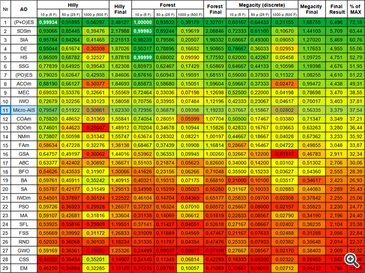
Starting from the previous article I have moved to absolute values of test results. So now it is very easy to navigate and compare the results of different algorithms in a table. 37.54% is not an outstanding result, but it is still a position in the top half of the table.

Visualization of the optimization process showed that the algorithm is persistent in exploring significant local extrema to achieve a better solution. This leads to the concentration of agents in different areas of space. The convergence graph showed unusual behavior. Typically, in the considered algorithms, there is a sharp increase in convergence in the first half of the iterations, and then the rate of convergence gradually decreases. However, in this algorithm the convergence graph is S-shaped. A sharp increase in convergence is observed only in the first 10-20% of iterations, then the speed of convergence decreases, but closer to the end of the optimization a significant acceleration in convergence can be seen again.

This behavior of the convergence graph can be explained by the strategy of narrowing the range of increments during mutations according to a linear law. However, convergence does not occur according to a linear law due to the uneven “accumulation” of information by the algorithm about the surface of the test function. Narrowing the mutation range begins to play a more noticeable role only closer to the end of optimization. Replacing the linear law of narrowing the range of mutations with other variants of nonlinear laws did not lead to an improvement in convergence, but perhaps there is room for the constructive imagination of researchers in choosing other variants of the laws of narrowing the range.

The convergence graph leaves much to be desired, however, its appearance gives hope that there is potential for further improvement of the search strategy.

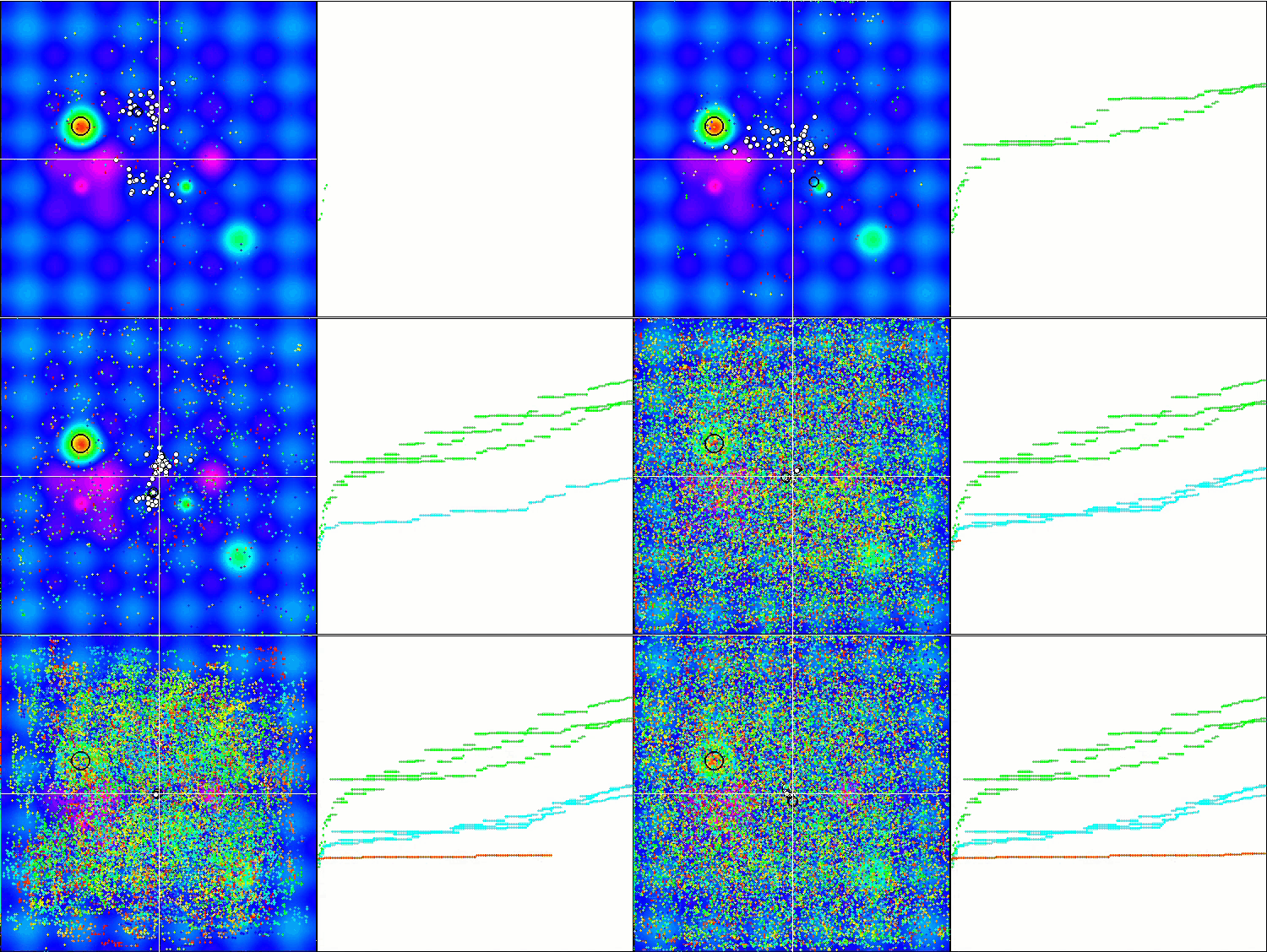
  Micro-AIS on the Hilly test function

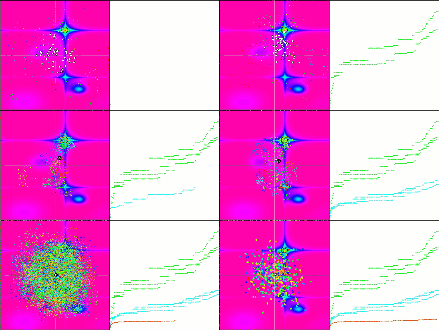
  Micro-AIS on the Forest test function

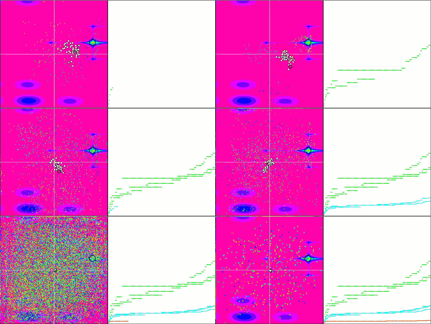
  Micro-AIS on the Megacity test function

The Micro-AIS algorithm took its rightful place on the 11th line of the rating table, ahead of such well-known and popular algorithms as the cuckoo optimization algorithm, artificial bee colony and simulated annealing. This indicates the efficiency of this algorithm in solving complex optimization problems.

However, according to the color table, we can notice a decrease in performance on functions with a large number of variables, which indicates the algorithm’s weak ability to scale. This may happen due to the fact that Micro-AIS uses a simpler model of the immune system and simpler immune information processing operations, which may limit its ability to find optimal solutions in high-dimensional spaces.

However, this does not mean that Micro-AIS cannot be used to solve problems with a large number of variables. Perhaps, its performance could be improved by modifying the algorithm or combining it with other optimization methods.

#	AO	Description	Hilly			Hilly final	Forest			Forest final	Megacity (discrete)			Megacity final	Final result	% of MAX
			10 p (5 F)	50 p (25 F)	1000 p (500 F)		10 p (5 F)	50 p (25 F)	1000 p (500 F)		10 p (5 F)	50 p (25 F)	1000 p (500 F)
1	(P+O)ES	(P+O) evolution strategies	0.99934	0.91895	0.56297	2.48127	1.00000	0.93522	0.39179	2.32701	0.83167	0.64433	0.21155	1.68755	6.496	72.18
2	SDSm	stochastic diffusion search M	0.93066	0.85445	0.39476	2.17988	0.99983	0.89244	0.19619	2.08846	0.72333	0.61100	0.10670	1.44103	5.709	63.44
3	SIA	simulated isotropic annealing	0.95784	0.84264	0.41465	2.21513	0.98239	0.79586	0.20507	1.98332	0.68667	0.49300	0.09053	1.27020	5.469	60.76
4	DE	differential evolution	0.95044	0.61674	0.30308	1.87026	0.95317	0.78896	0.16652	1.90865	0.78667	0.36033	0.02953	1.17653	4.955	55.06
5	HS	harmony search	0.86509	0.68782	0.32527	1.87818	0.99999	0.68002	0.09590	1.77592	0.62000	0.42267	0.05458	1.09725	4.751	52.79
6	SSG	saplings sowing and growing	0.77839	0.64925	0.39543	1.82308	0.85973	0.62467	0.17429	1.65869	0.64667	0.44133	0.10598	1.19398	4.676	51.95
7	(PO)ES	(PO) evolution strategies	0.79025	0.62647	0.42935	1.84606	0.87616	0.60943	0.19591	1.68151	0.59000	0.37933	0.11322	1.08255	4.610	51.22
8	ACOm	ant colony optimization M	0.88190	0.66127	0.30377	1.84693	0.85873	0.58680	0.15051	1.59604	0.59667	0.37333	0.02472	0.99472	4.438	49.31
9	MEC	mind evolutionary computation	0.69533	0.53376	0.32661	1.55569	0.72464	0.33036	0.07198	1.12698	0.52500	0.22000	0.04198	0.78698	3.470	38.55
10	IWO	invasive weed optimization	0.72679	0.52256	0.33123	1.58058	0.70756	0.33955	0.07484	1.12196	0.42333	0.23067	0.04617	0.70017	3.403	37.81
11	Micro-AIS	micro artificial immune system	0.79547	0.51922	0.30861	1.62330	0.72956	0.36879	0.09398	1.19233	0.37667	0.15867	0.02802	0.56335	3.379	37.54
12	COAm	cuckoo optimization algorithm M	0.75820	0.48652	0.31369	1.55841	0.74054	0.28051	0.05599	1.07704	0.50500	0.17467	0.03380	0.71347	3.349	37.21
13	SDOm	spiral dynamics optimization M	0.74601	0.44623	0.29687	1.48912	0.70204	0.34678	0.10944	1.15826	0.42833	0.16767	0.03663	0.63263	3.280	36.44
14	NMm	Nelder-Mead method M	0.73807	0.50598	0.31342	1.55747	0.63674	0.28302	0.08221	1.00197	0.44667	0.18667	0.04028	0.67362	3.233	35.92
15	FAm	firefly algorithm M	0.58634	0.47228	0.32276	1.38138	0.68467	0.37439	0.10908	1.16814	0.28667	0.16467	0.04722	0.49855	3.048	33.87
16	GSA	gravitational search algorithm	0.64757	0.49197	0.30062	1.44016	0.53962	0.36353	0.09945	1.00260	0.32667	0.12200	0.01917	0.46783	2.911	32.34
17	ABC	artificial bee colony	0.63377	0.42402	0.30892	1.36671	0.55103	0.21874	0.05623	0.82600	0.34000	0.14200	0.03102	0.51302	2.706	30.06
18	BFO	bacterial foraging optimization	0.54626	0.43533	0.31907	1.30066	0.41626	0.23156	0.06266	0.71048	0.35500	0.15233	0.03627	0.54360	2.555	28.39
19	BA	bat algorithm	0.59761	0.45911	0.35242	1.40915	0.40321	0.19313	0.07175	0.66810	0.21000	0.10100	0.03517	0.34617	2.423	26.93
20	SA	simulated annealing	0.55787	0.42177	0.31549	1.29513	0.34998	0.15259	0.05023	0.55280	0.31167	0.10033	0.02883	0.44083	2.289	25.43
21	IWDm	intelligent water drops M	0.54501	0.37897	0.30124	1.22522	0.46104	0.14704	0.04369	0.65177	0.25833	0.09700	0.02308	0.37842	2.255	25.06
22	PSO	particle swarm optimisation	0.59726	0.36923	0.29928	1.26577	0.37237	0.16324	0.07010	0.60572	0.25667	0.08000	0.02157	0.35823	2.230	24.77
23	MA	monkey algorithm	0.59107	0.42681	0.31816	1.33604	0.31138	0.14069	0.06612	0.51819	0.22833	0.08567	0.02790	0.34190	2.196	24.40
24	SFL	shuffled frog-leaping	0.53925	0.35816	0.29809	1.19551	0.37141	0.11427	0.04051	0.52618	0.27167	0.08667	0.02402	0.38235	2.104	23.38
25	FSS	fish school search	0.55669	0.39992	0.31172	1.26833	0.31009	0.11889	0.04569	0.47467	0.21167	0.07633	0.02488	0.31288	2.056	22.84
26	RND	random	0.52033	0.36068	0.30133	1.18234	0.31335	0.11787	0.04354	0.47476	0.25333	0.07933	0.02382	0.35648	2.014	22.37
27	GWO	grey wolf optimizer	0.59169	0.36561	0.29595	1.25326	0.24499	0.09047	0.03612	0.37158	0.27667	0.08567	0.02170	0.38403	2.009	22.32
28	CSS	charged system search	0.44252	0.35454	0.35201	1.14907	0.24140	0.11345	0.06814	0.42299	0.18333	0.06300	0.02322	0.26955	1.842	20.46
29	EM	electroMagnetism-like algorithm	0.46250	0.34594	0.32285	1.13129	0.21245	0.09783	0.10057	0.41085	0.15667	0.06033	0.02712	0.24412	1.786	19.85

Summary

The micro artificial immune system (Micro-AIS) optimization method is an interesting and promising approach to solving optimization problems based on the principles of the immune system functioning. It allows using the powerful mechanism of the immune system to solve complex optimization and learning problems.

Among the advantages of Micro-AIS are a small number of external parameters and a simple implementation of the algorithm. This makes it quite attractive for use in practical tasks.

However, the Micro-AIS algorithm also has disadvantages. It is prone to getting stuck at local extremes and has low convergence. Moreover, the algorithm performance decreases on functions with a large number of variables, which indicates its weak scaling ability.

However, Micro-AIS is a promising optimization method that can be improved by modifying the algorithm or combining with other optimization methods. Overall, the optimization method using artificial micro-immune system is an important contribution to the field of optimization and can be a useful tool in solving complex problems in various fields such as machine learning, artificial intelligence, bioinformatics, etc.

The algorithm leaves the impression of being a kind of a "template" that can be built on using various methods and expand the search capabilities. This is facilitated by the simple architecture, which leaves really huge scope for experimenting with this very interesting algorithm.

Figure 1. Color gradation of algorithms according to relevant tests

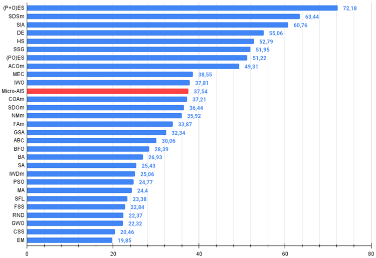
Figure 2. The histogram of algorithm test results (on a scale from 0 to 100, the more the better,

where 100 is the maximum possible theoretical result (the archive features a script for calculating the rating table)

Micro-AIS algorithm pros and cons:

Advantages:

1. Small number of external parameters.
2. Simple algorithm implementation.

Disadvantages:

1. Tendency to get stuck.
   
2. Low convergence.
   

The article is accompanied by an archive with updated current versions of the algorithm codes described in previous articles. The author of the article is not responsible for the absolute accuracy in the description of canonical algorithms. Changes have been made to many of them to improve search capabilities. The conclusions and judgments presented in the articles are based on the results of the experiments.