Building a Trading System (Part 4): How Random Exits Influence Trading Expectancy

Introduction

In Part 3 of this series, we explored how traders can set realistic profit targets and achieve their goals using system statistics. We established that each win-rate and reward-to-risk ratio (RRR) requires a unique combination of position sizing and trade frequency to reach long-term trading objectives. While multiple-entry strategies can help increase trade volume, there is a crucial concept to examine before we move further—random win-rate management.

Many traders have once experienced this trading path, follow a defined entry strategy but often struggle with managing open positions. It is common to enter a trade based on solid analysis, only to panic once price begins to fluctuate. This often leads to closing trades prematurely, either before take profit or stop loss is reached. Over time, this behavior erodes the equity curve, creating a consistent downward slope.

This raises important questions:

• How can traders avoid this destructive pattern?
• Is it possible to exit trades before reaching a set profit target and still grow account equity?
• Can randomness in profit-taking be structured in a way that improves results?

In this article, we explore these questions using Monte Carlo simulation to model outcomes when traders exit trades at random profit levels. By understanding this approach, traders can design systems that remain profitable even when profits are taken inconsistently. 

Understanding Random Win-Rate

In Part 1 of this series, we demonstrated that every fixed RRR corresponds to a minimum win-rate threshold that must be exceeded to achieve profitability. For example:

• At RRR = 1.5, the minimum win-rate is 40%.
• For RRR = 2.5, the minimum win-rate drops to 28.6%.
• Given RRR = 3.0, profitability requires at least 25% wins.

When a trader consistently applies a fixed RRR, the math is straightforward: profitability hinges on maintaining a win-rate above the threshold.

However, in practice, many traders exit trades at random profit levels, whether due to fear, impatience, or trailing-stop mechanisms. This behavior introduces variable RRRs, which in turn generate variable win-rates.

Consider an example:

• First 50 trades: 45% win-rate at RRR = 1.2
• Next 50 trades: 60% win-rate at RRR = 0.3
• Final 50 trades: 30% win-rate at RRR = 2.0

In total, the trader executed 150 trades, each with different win-rates and RRRs. The critical question: Is the trader profitable overall?

The answer lies in calculating the expectancy of the trading system.

Expectancy Formula

Expectancy measures the average return per trade and determines whether a system is profitable:

• If E > 0, the system is profitable.
• If E ≤ 0, the system is unprofitable.

By summing the expectancy across trades with different RRRs and win-rates, traders can evaluate whether their random exits still generate net positive results.

Random Win-Rate Through Volatility Stops

Another form of random win-rate emerges when traders use volatility-based trailing stops. Tools such as:

• Average True Range (ATR)
• Standard Deviation
• Bollinger Bands

just to mention a few dynamically adjust stop-loss levels based on market volatility.

At times of high volatility (e.g., 1000 points), trades may remain open longer possibly hinting profits or exiting at higher RRRs. Conversely, during low volatility (e.g., 200 points), trades may be cut short prematurely, reducing RRRs. This naturally generates random outcomes, as RRR fluctuates depending on market conditions.

Such randomness introduces both risks and opportunities. On one hand, traders may secure small profits too early. On the other, they may capture large moves during periods of strong volatility. The challenge is to balance these outcomes in a way that maintains positive expectancy.

Monte Carlo Simulation: Analyzing Random Win-Rates

To better understand how random exits impact profitability, we will employ Monte Carlo simulation in the next section. By modeling hundreds to thousands of random trade outcomes, we can observe how expectancy behaves under different scenarios of random RRRs and win-rates.

This analysis will provide actionable insights into:

• How random exits affect long-term equity curves.
• Whether traders can improve results by embracing randomness strategically.
• Practical adjustments to design profitable systems under real-world conditions.

Case Study: Evaluating Trade Management Through Random Win-Rates

In this study, we examine a trading system with a 30% win-rate at a fixed RRR of 4. Three traders employed this system but, due to 15 consecutive losses, they decided to modify their exit strategies by taking profits at five different RRR levels.

Trader 1: Profile and Expectancy

We will analyze Trader 1’s performance, his equity curve outcomes, drawdowns, and combined strategies using Monte Carlo simulations. Table 1 summarizes Trader 1’s trading results at different win-rates and RRR levels, along with expectancy values:

Table 1: Trader 1's trading profile

Win Rate (%)	RRR	Expectancy
20.92%	2.61	-0.244
36.22%	2.15	0.142
51.91%	1.84	0.475
61.24%	0.55	-0.049
76.55%	0.27	-0.029

Analysis shows that three strategies (20.9%, 61.2%, and 76.6% win-rates) generate negative expectancy, while two strategies (36.2% and 51.9%) show positive expectancy. However, because the cumulative sum of expectancy is positive, this trader can still achieve overall profitability if the strategy mix is managed effectively.

Trader 1: Visual Inspection of Equity Curves

Using 100 trades per system, we observed the following:

• Negative expectancy strategies (20.9%, 61.2%, 76.6% win-rates) produced declining equity curves.
• Positive expectancy strategies (36.2% and 51.9% win-rates) produced rising equity curves.

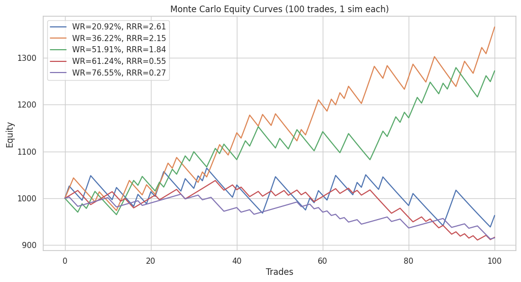
Figure 1: Trader 1's trading system

To quantify performance, we ran 100 simulations per strategy and analyzed equity and drawdown outcomes via box-plots.

Drawdown Analysis for Trader 1

For Trader 1, the analysis of risk and return profiles reveals a significant variation in potential drawdowns depending on the win-rate and RRR. The maximum drawdown is recorded at a win-rate of 51.9% with an RRR of 1.84, where losses can exceed 55% of account equity. Conversely, the minimum drawdown occurs at a win-rate of 76.5% with an RRR of 0.27, where losses are contained to below 5%.

All other combinations of win-rates and their corresponding RRR values for Trader 1 fall within these two extremes, indicating that the risk exposure ranges between a very mild equity reduction and a potentially severe capital drawdown.

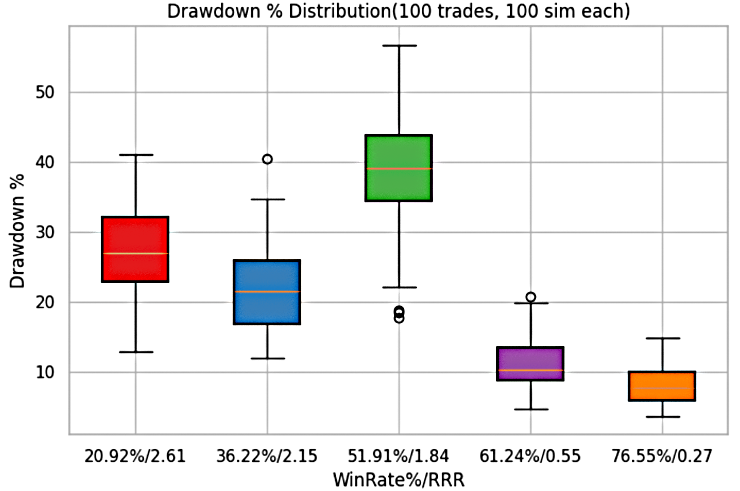
Figure 2: Trader 1's drawdown% for each system

Equity Curve Analysis for Trader 1

The assessment of Trader 1’s performance also extends to the behavior of the equity curve under varying win-rates and RRR. The maximum equity curve is associated with a 51.9% win-rate and an RRR of 1.84, where account growth rises to slightly above $2,000. On the other hand, the minimum equity curve is observed at a 20.9% win-rate with an RRR of 2.61, where the account value drops below $500.

All other potential equity curves generated under different win-rates and RRR combinations remain bounded between these two extremes, underscoring the wide variability of performance outcomes that depend on the underlying trading parameters.

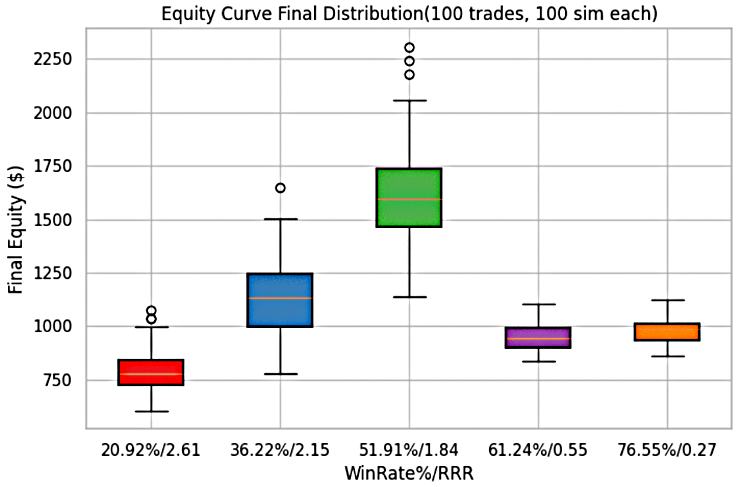
Figure 3: Trader 1's equity curves for each system

Table 2 provides summarized view of the figure 2 & 3.

Table 2: Mean & Median equity and Median drawdown for Trader 1

Win Rate (%)	RRR	Mean Equity ($)	Median Equity ($)	Median Drawdown (%)
20.92%	2.61	$789.00	$777.00	26.99%
36.22%	2.15	$1130.00	$1132.00	21.57%
51.91%	1.84	$1601.00	$1596.00	39.03%
61.24%	0.55	$950.00	$946.00	10.29%
76.55%	0.27	$978.00	$988.00	7.77%

Key Insight:

• The highest median equity ($1,595) is achieved at 51.9% win-rate with RRR = 1.84, though this comes with the highest median drawdown (39%).
• The lowest drawdown (7.8%) occurs at 76.5% win-rate with RRR = 0.27, but equity is capped below $1,000.
• The weakest performer is the 20.9% win-rate with RRR = 2.61, where both equity and expectancy are negative, making it a drag on overall performance.

Combined Trade Management Strategy -->Trader 1

To simulate real trading conditions, we ran 500 Monte Carlo simulations in which any of the five strategies could be randomly applied across 100 trades. 

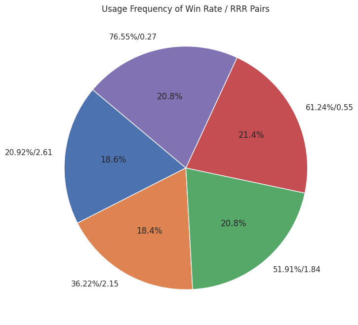
Figure 4: Trader 1's Integrated Trade Management Approach

A pie chart of Trader 1’s performance reveals how different trade management strategies were applied throughout his trading journey. The allocation was relatively balanced across the five approaches:

• 20.9% win-rate system → 18.6% of trades
• 36.2% win-rate system → 18.4% of trades
• 51.9% win-rate system → 20.8% of trades
• 61.2% win-rate system → 21.4% of trades
• 76.5% win-rate system → 20.8% of trades

This near-even distribution shows that Trader 1 did not rely excessively on any single approach, but instead diversified execution across multiple systems.

The combined effect of these strategies is illustrated in Figure 5 for both equity growth and drawdowns . These visualizations highlight the range of possible outcomes when the systems are blended together, demonstrating how diversification reduces risk exposure while moderating maximum equity gains.

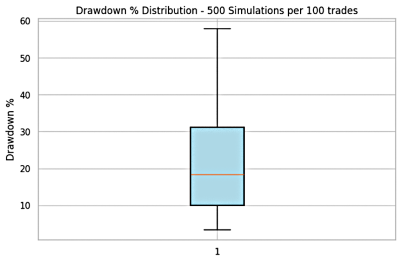
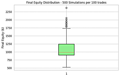
Figure 5: Combined Strategy Result of Trader 1 

Table 3: Combined Results for Trader 1

Mean Equity ($)	Median Equity ($)	Median Drawdown (%)
$1092.00	$991.00	18.38%

Key Insight

• Drawdowns ranged from below 5% (76.5% win-rate system influence) to above 55% (51.9% win-rate system influence).
• Equity curves ranged from a minimum near $500 to a maximum around $1,750.
• The probability of achieving the $2,000 mark was reduced compared to using the 51.9% win-rate system alone.
• The mean equity ($1,091) and median equity ($990) suggest stable but moderate account growth.
• The median drawdown (18.4%) is significantly lower than the worst-case single system (39–55%), highlighting reduced risk through diversification.

Optimizing the Strategy : Trader 1

To enhance profitability, Trader 1 should:

1. Increase reliance on the 36.2% win-rate at RRR = 2.15, which shows strong expectancy, controlled drawdown (~21.6%), and equity potential near $1,500.
2. Reduce or eliminate the 20.9% win-rate at RRR = 2.61, which consistently produces negative expectancy and weak equity outcomes.
3. Consider weighted allocation toward higher expectancy systems rather than equal distribution to improve the balance between growth and risk.

Trader 2: Profile and Expectancy

Trader 2’s trading profile is built on five different risk-reward ratios (RRR) and their corresponding win rates. The expectancy values associated with each are shown in Table 4:

Table 4: Trader 2's trading profile

Win Rate (%)	RRR	Expectancy
21.46%	2.98	-0.147
36.65%	1.80	0.026
55.09%	1.28	0.256
56.41%	1.11	0.188
77.38%	0.78	0.379

From Table 4, it is clear that only one system—the 21.5% win-rate with RRR=2.98—carries a negative expectancy. The remaining four methods all have positive expectancy, with particularly strong potential at 55.1% and 77.4% win rates. This suggests that Trader 2, when applying this diversified plan, has a high probability of achieving positive long-term results.

Trader 2: Visual Inspection of Equity Curves

A visual inspection of equity curves across 100 trades reveals distinct patterns:

• The 21.5% win-rate system predictably shows a declining curve, consistent with its negative expectancy.
• The 36.7% and 56.4% win-rate systems demonstrate sluggish growth, hovering around the break-even range of $1,000–$1,100.
• The 55.1% and 77.4% win-rate systems exhibit robust upward equity curves, making them the strongest contributors to profitability.

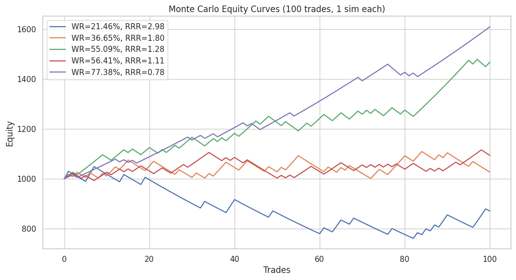
Figure 6: Trader 2's trading system

To assess statistical reliability, 100 simulations were conducted for each system, and their performance was analyzed via equity and drawdown box plots.

Drawdown Analysis for Trader 2

Similar to Trader 1, each trading system presents its own range of drawdowns depending on the interaction between win-rate and RRR. For Trader 2, the maximum drawdown is observed at a 77.4% win-rate with an RRR of 0.78, where losses approach 45% of account equity. The minimum drawdown occurs at a 56.4% win-rate and an RRR of 1.11, where losses are contained to around 5%.

All other win-rate and RRR combinations for Trader 2 produce drawdowns that lie between these upper and lower limits, reinforcing the pattern that system-specific risk exposures are highly sensitive to parameter variations.

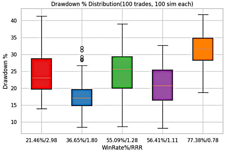
Figure 7:  Trader 2's drawdown% for each system

Equity Curve Analysis for Trader 2

In Trader 2’s trading approach, the maximum equity curve is achieved at a 77.4% win-rate with an RRR of 0.78, where account growth rises to slightly above $1,700. Conversely, the minimum equity curve is observed at a 21.5% win-rate with an RRR of 2.98, where equity declines to below $600.

All other equity curves generated under the remaining win-rate and RRR combinations lie within these two boundaries, demonstrating the sensitivity of performance outcomes to the balance between probability of success and risk-reward trade-offs.

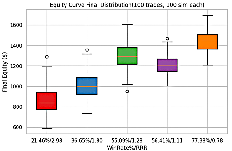
Figure 8: Trader 2's equity curves for each system

Table 5 summarizes the key findings from Figures 7 and 8.

Table 5: Mean & Median equity and Median drawdown for Trader 2

Win Rate (%)	RRR	Mean Equity ($)	Median Equity ($)	Median Drawdown (%)
21.46%	2.98	$858.00	$837.00	23.11%
36.65%	1.80	$1008.00	$999.00	17.11%
55.09%	1.28	$1295.00	$1295.00	25.62%
56.41%	0.11	$1214.00	$1202.00	20.76%
77.38%	0.78	$1442.00	$1445.00	31.66%

Key Insight

• The highest equity growth is achieved with the 77.4% win-rate system (mean equity ≈ $1,443).
• The lowest performance comes from the 21.5% win-rate system (mean equity ≈ $858).
• Median drawdowns vary considerably, from a low of approximately 17% (36.7% win-rate) to highs above 30% (77.4% win-rate).
• While higher win-rate strategies deliver stronger growth, they also tend to carry deeper drawdowns.

Combined Trade Management Strategy -->Trader 2

A 500-trial Monte Carlo simulation was conducted, randomly mixing the five strategies over 100 trades.

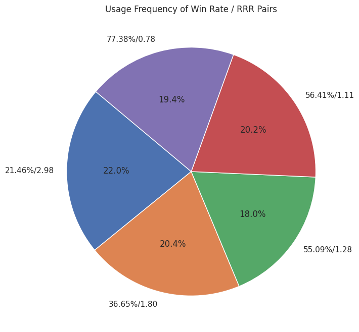
Figure 9: Trader 2's Integrated Trade Management Approach

The results reveal the distribution of how Trader 2 applied his methods:

• 21.5% win-rate system → 22.0% of trades
• 36.7% win-rate system → 20.4% of trades
• 55.1% win-rate system → 18.0% of trades
• 56.4% win-rate system → 20.2% of trades
• 77.4% win-rate system → 19.4% of trades

This distribution reflects a diversified approach, ensuring no single strategy dominates the overall results.

The combined results of these strategies is shown in Figure 10 for both equity growth and drawdowns.

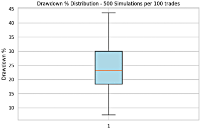
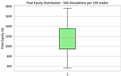
Figure 10: Combined Strategy Result of Trader 2 

 

Table 6: Combined Results for Trader 1

Mean Equity ($)	Median Equity ($)	Median Drawdown (%)
$1167.00	$1169.00	23.14%

Key Insight

• Drawdowns ranged from 5% to 45%, mirroring the extremes of the best and worst systems.
• Equity curves spanned between $600 and $1,800, with the maximum equity boosted by diversification compared to weaker individual systems.
• The 36.7% and 56.4% systems provide stability but contribute little to equity expansion.
• Achieving $2,000 equity after 100 trades was statistically unlikely, as this fell outside the maximum observed values.

Optimizing the Strategy : Trader 2

To enhance profitability strategically, Trader 2 may consider:

1. Allocating more weight to the 55.1% win-rate (RRR=1.28) system, which offers a favorable balance of growth and manageable drawdowns,
2. Reducing reliance on the 21.5% win-rate (RRR=2.98) strategy, which consistently drags performance downward.

Trader 3: Profile and Expectancy

Trader 3’s trading profile consists of five distinct trade management strategies, each defined by its win rate, RRR, and expectancy:

Table 7: Trader 3's trading profile

Win Rate (%)	RRR	Expectancy
39.64%	2.93	0.556
41.55%	1.58	0.074
52.51%	1.53	0.331
58.29%	1.24	0.305
60.36%	0.43	-0.139

From this breakdown, we observe that four strategies generate positive expectancy, while only one—the 60.4% win-rate with RRR=0.43—has a negative expectancy. Since the cumulative expectancy across all strategies is positive, Trader 3’s overall trading plan has a strong chance of producing profitable results.

Trader 3: Visual Inspection of Equity Curves

To evaluate performance, we simulated 100 trades for each strategy. A visual inspection of equity curves is shown in Figure 11:

• Negative expectancy strategy (60.4% win rate, RRR=0.43): Produces a steadily declining equity curve over time.
• Moderate positive expectancy Strategies (41.6%, 52.5%, 58.3% win rate): Show steady equity growth, though with varying volatility.
• High RRR strategy (39.6% win rate, RRR=2.93): Exhibits the strongest equity growth, but also the sharpest fluctuations, with large swings up and down.

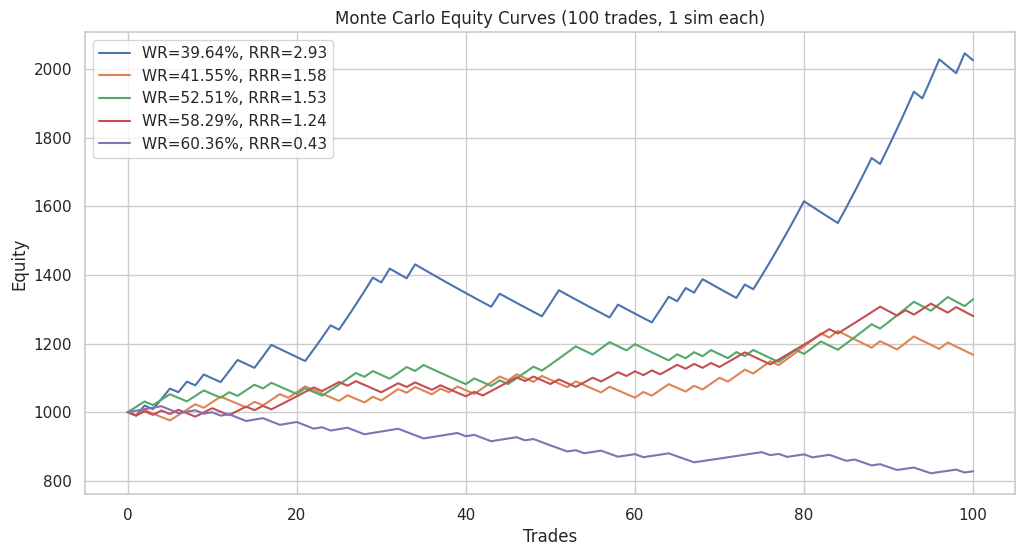
Figure 11: Trader 3's trading system

To assess statistical reliability, 100 simulations were conducted for each system, and their performance was analyzed via equity and drawdown box plots.

Drawdown Analysis for Trader 3

As demonstrated in the cases of Trader 1 and Trader 2, each trading system generates a unique drawdown profile shaped by the relationship between win-rate and RRR. For Trader 3, the maximum drawdown occurs at a 39.6% win-rate with an RRR of 2.93, where losses reach approximately 65% of account equity. In contrast, the minimum drawdown is recorded at a 60.4% win-rate with an RRR of 0.43, where equity reduction is limited to about 5%.

All other win-rate and RRR combinations for Trader 3 fall within these two extremes, confirming that system performance is tightly bound by the interplay of probability and risk-reward dynamics.

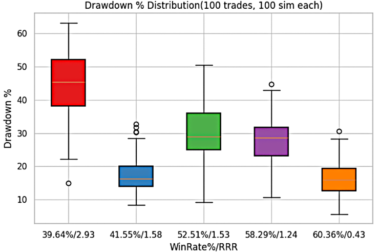
Figure 12: Trader 3's drawdown% for each system

Equity Curve Analysis for Trader 3

In Trader 3’s trading method, the maximum equity curve is achieved at a 39.6% win-rate with an RRR of 2.93, where account growth rises to approximately $2,700. On the other hand, the minimum equity curve is observed at a 60.4% win-rate with an RRR of 0.43, where equity falls to about $750.

The equity curves from all remaining win-rate and RRR combinations remain within these two bounds, highlighting the variability in outcomes that depend on the chosen balance between probability of success and reward-to-risk trade-offs.

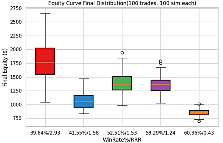
Figure 13: Trader 3's equity curves for each system

Table 8 provides a summarized view of Figures 12 & 13.

Table 8: Mean & Median equity and Median drawdown for Trader 3

Win Rate (%)	RRR	Mean Equity ($)	Median Equity ($)	Median Drawdown (%)
39.64%	2.93	$1775.00	$1768.00	45.41%
41.55%	1.58	$1080.00	$1053.00	16.34%
52.51%	1.53	$1387.00	$1363.00	28.93%
58.29%	1.24	$1353.00	$1369.00	28.55%
60.36%	0.43	$861.00	$852.00	16.03%

Key Insight:

• The 39.6% win-rate system provides the highest mean and median equity, but also the largest drawdowns.
• The 52.5% and 58.3% win-rate systems achieve solid equity growth while keeping drawdowns under 50%, making them more sustainable.
• The 60.4% win-rate strategy drags performance down due to its negative expectancy.

Combined Trade Management Strategy -->Trader 3

A 500-trial Monte Carlo simulation was conducted, randomly mixing the five strategies over 100 trades.

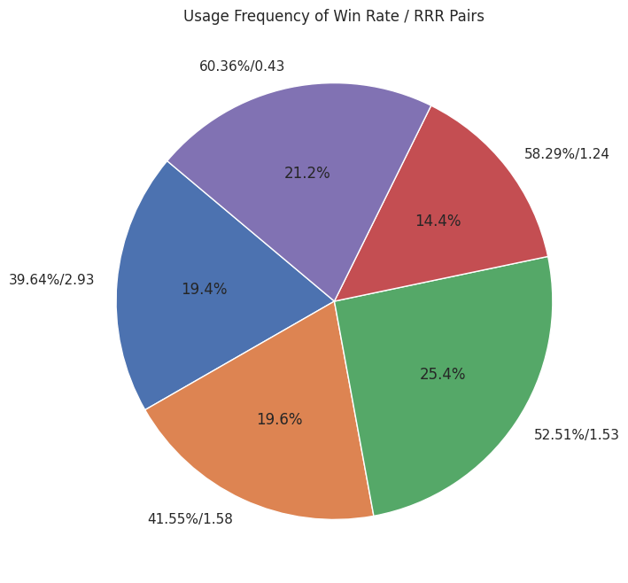
Figure 14: Trader 3's Integrated Trade Management Approach

The allocation of strategies was as follows:

• 19.4% → 39.6% win-rate system
• 19.6% → 41.6% win-rate system
• 25.4% → 52.5% win-rate system
• 14.4% → 58.3% win-rate system
• 21.2% → 60.4% win-rate system

This distribution represents a diversified approach, introducing a degree of intentional imbalance in strategy allocation designed to enhance the overall performance.

The combined outcomes of these strategies—covering both equity growth and drawdown patterns—are presented in Figure 15.

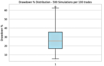
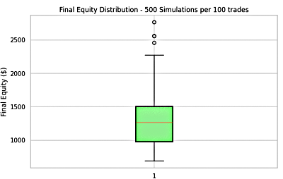
Figure 15: Combined Strategy Result of Trader 3

Table 9: Combined Results for Trader 3

Mean Equity ($)	Median Equity ($)	Median Drawdown (%)
$1291.00	$1263.00	25.48%

Key Insight:

• Drawdowns: Spanning from 5% to 65%, mirroring the extremes of single-system performance. The median drawdown of 25.48% indicates a moderate yet manageable risk profile, highlighting stronger control compared to higher-risk individual systems.
• Equity Curves: Fluctuate between a low of $400 and a high of $2,250. The mean equity ($1,290.77) and median equity ($1,263.45) are closely aligned, suggesting consistent profitability across simulations, with performance shaped by stable outcomes rather than outliers.
• Combined Strategy Impact: While the maximum equity is lower than the strongest single system ($2,700 at a 39.6% win rate), the combined approach smooths growth, reduces volatility, and delivers a balanced result that still surpasses $2,000.

Optimizing the Strategy : Trader 3

1. Increase allocation to the 52.5% and 58.3% win-rate systems, which offer sustainable equity growth with drawdowns below 50%.
2. Reduce or eliminate the 60.4% win-rate system, since its negative expectancy erodes profitability.
3. Reduce the 39.6% win-rate strategy—while highly profitable, its extreme drawdowns pose significant risk if not managed with strict position sizing.

Code Structure

The following lines of code serve as inputs to generate other trading scenarios. 

# Initial parameters
initial_equity = 1000
risk_per_trade = 0.01  # 1% risk
trades_per_run = 100

# Step 1: Generate 5 random win-rates (10%-95%) and 5 random RRR (0.1 - 5)
np.random.seed(94)
win_rates = np.random.uniform(0.10, 0.80, 5)
rrr = np.random.uniform(0.1, 3, 5)

• Initial Parameters
• initial_equity= 1000 :  This sets the starting account balance at $1,000. All subsequent trades will build on this base value, allowing us to measure growth, losses, and drawdowns.
• risk_per_trade= 0.01:  The trader risks 1% of equity per trade. If equity is $1,000, each trade carries a $10 risk. This variable controls position sizing and helps simulate realistic money management.
• trades_per_run = 100 :  Each Monte Carlo run simulates 100 trades. This provides a statistical sample large enough to observe trends, streaks of wins or losses, and long-term expectancy.

• To explore multiple trading environments, the code generates random win-rates and RRR.
• np.random.seed(42):  Sets the random seed so that the simulation is reproducible. Every time the code runs, the same random numbers are generated, ensuring consistent results. It should be commented out to allow for different possible randomness or changing the seed value.
• win_rates = np.random.uniform(0.10, 0.80, 5) : Produces five random win rates between 10% and 80%.
• rrr = np.random.uniform(0.1, 3, 5) : Produces five random reward-to-risk ratios between 0.1 and 3.0.

To replicate the trading scenarios presented for Trader 1, Trader 2, and Trader 3, the reader can modify the seed number used for generating random values within the python code. The following seed values were used for each scenario:

• Trader 1: Seed value = 42
• Trader 2: Seed value = 30
• Trader 3: Seed value = 94

By applying these seed values and re-running the code, readers can reproduce the different trading outcomes observed in the simulations, demonstrating how randomness in take profit levels influences overall performance.

Building the Strategy: Demonstrating Random Take Profit Levels

To better understand the concept of random take profit levels while maintaining a fixed stop loss and consistent entry setup, we developed a simple trading strategy to illustrate this idea in practice. The strategy combines two well-known technical indicators — the Parabolic SAR and the DeMarker indicator — to identify potential trade entries.

For broader accessibility, this Expert Advisor (EA) has been developed for both MetaTrader 4 and MetaTrader 5 platforms. In this section, we will focus on the MetaTrader 5 version and provide a brief walkthrough of its code structure to help readers understand how the concept is implemented in practice.

// Input parameters
input double   LotSize=0.01;            // Lot Size
input double   pStep = 0.01;            // Psar Step
input double   pMax = 0.1;              // Psar Max
input int      DemPeriod = 14;          // DeMarker Period
input double   Overbought = 0.7;        // Overbought >0.5 & < 1
input int      StopLoss=50;             // Stop Loss (pips)
input int      MinRandomTP = 30;        // MinRandom TakeProfit (pips)
input int      MaxRandomTP=200;         //MaxRandom TakeProfit

double OverSold = 1- Overbought;

The input parameters are designed to provide flexibility, allowing traders to adjust the settings to their preferred trading conditions without modifying the core code. Each parameter serves a specific purpose in defining the behavior of the trading strategy.

• Lot Size: The Lotsize parameter determines the trade volume or the amount of capital the trader is willing to risk per position. By default, this is set to 0.01 lots, making it suitable for conservative trading or testing.

• pStep and pMax: The pStep and pMax parameters control the acceleration factor and maximum acceleration of the Parabolic SAR indicator. These values influence how quickly the SAR reacts to price changes. The default values are 0.01 for pStep and 0.1 for pMax, providing a balanced sensitivity for trend-following setups.

• DemPeriod: The DemPeriod parameter specifies the period used by the DeMarker indicator to calculate its values. The default setting is 14.

• Overbought and Oversold Levels:  The Overbought parameter defines the upper threshold for the DeMarker indicator, marking potential reversal zones. It should be set between 0.5 and 1.0. The Oversold level is automatically calculated as 1 – Overbought, ensuring a symmetrical range between the two conditions.

• Stoploss: The Stoploss parameter specifies the risk limit per trade, expressed in pips. It is automatically converted to points when necessary by the system. The default stop loss is set at 50 pips, providing a moderate buffer against market volatility.

• MinRandomTP and MaxRandomTP: The MinRandomTP and MaxRandomTP parameters define the minimum and maximum bounds for take profit levels. These values are passed to a function that generates a random take profit within the specified range. By default, the minimum is 30 pips and the maximum is 200 pips, allowing for varied profit targets that simulate dynamic market conditions.

//---Time to start and end trade
double startTrade = 1;   //StartTradeTime(hrs)
double endTrade = 22;    // EndTradeTime(hrs)

bool IsTimeToTrade()
  {
   MqlDateTime brokertime_struct;
   TimeCurrent(brokertime_struct);
   double brokertime = brokertime_struct.hour;

   return (brokertime > startTrade && brokertime <= endTrade) ? true : false;
  }

The trading system operates within a specific time window to ensure trades are executed only during active market hours. In this setup, the time interval is set between 1 and 22 hours of the trading day.

The function, IsTimeToTrade(), verifies whether the current market time falls within the predefined trading window. If the condition is met, trading operations are allowed to proceed; otherwise, the system pauses to prevent entries during inactive or volatile off-market hours.

Generating Random Take Profit Levels

//--- Seed random generator once when EA is loaded
   MathSrand(TimeCurrent());

During the initialization phase of the EA, the random number generator is seeded using the TimeCurrent() function. This ensures that each execution of the trading algorithm produces unique random values, particularly for generating random take profit levels, rather than repeating the same sequence on every run.

By linking the random seed to the current market time, the system introduces natural variability into trade outcomes, allowing for a more realistic simulation of dynamic trading conditions.

int RandomTakeProfit(int min, int max)
  {
// Normalize MathRand() into 0.0 – 1.0
   double rnd = (double)MathRand() / 32767.0;

// Scale to desired range [min, max]
   int result = (int)MathRound(min + rnd * (max - min));
   Print("TPValues: ",result);
   return result;
  }

The RandomTakeProfit() function is responsible for creating dynamic profit targets within a defined range. It accepts two input parameters — the minimum and maximum take profit values — and then generates a random take profit level between these limits for the EA to apply to each trade.

To enhance transparency and assist with performance monitoring, a Print() statement has been included in the code. This function outputs the randomly generated take profit value to the terminal for every trade opened, allowing traders to track and analyze how varying profit targets influence the overall system performance.

Defining the Entry Criteria

The trading system follows a simple yet effective rule-based approach that combines the Parabolic SAR and DeMarker indicators to determine entry signals.

//--- Sell condition
   bool sellSignal = psar[0] > high[0] ?
                     (demCurrent[0] > Overbought && demPrevious[0] < Overbought) ? true : false
                     : false;

//--- Buy condition
   bool buySignal = psar[0] < low[0] ?
                    (demCurrent[0] < OverSold && demPrevious[0] > OverSold) ? true : false
                    : false;

Sell Condition:
A sell trade is triggered when the Parabolic SAR indicator appears above the candle’s high, signaling potential downward pressure in price. At the same time, the DeMarker indicator must cross into the overbought region, confirming that the market may be overextended to the upside and ready for a retracement.

Buy Condition:
Conversely, a buy trade is initiated when the Parabolic SAR is positioned below the candle’s low, indicating potential upward momentum. The DeMarker indicator must simultaneously cross into the oversold region, suggesting that selling pressure is weakening and a bullish reversal may occur.

These combined conditions aim to filter out false signals and improve trade timing by aligning trend and momentum indicators.

Random Take Profit Results

A backtest was conducted on the GBPUSD pair using the H1 timeframe to evaluate the performance of the strategy under varying take profit conditions. During the test, each trade was executed using the same entry setup and fixed stop loss, while the take profit levels were randomly selected within the predefined range.

This approach produced a series of trades that, although identical in entry criteria and risk parameters, differed in their exit points. It is important to emphasize that even when trades share the same entry signals, varying exit conditions — in this case, random take profit levels — lead to distinct trading outcomes. This introduces diversity and dynamism into the Expert Advisor’s behavior, making it more adaptive to changing market conditions.

The results of the backtest are illustrated in Figures 16 and 17, which display the equity performance and trade distribution across the randomly generated take profit levels.

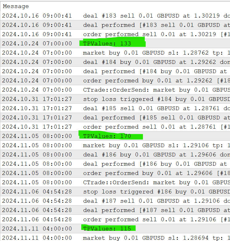
Figure 16: Random Take Profit level at Each Entry

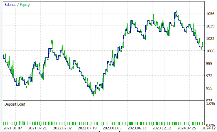
Figure 17: Random TP graph

Conclusion

Consistency in trading depends less on entry quality and more on structured exit management. Random, emotional exits destroy expectancy; quantified, rule-based variability can enhance it.

Tracking every exit and analyzing expectancy over large samples turns intuition into data. Profitability stems from expectancy, not from rigid profit targets — frequent smaller wins with a positive expectancy can outperform rare big ones.

Structured randomness, such as volatility-based trailing stops with back-tested minimum profit thresholds, can systematize uncertainty and preserve gains. Monte Carlo testing then validates these rules under varied market conditions, converting randomness into an advantage.

Next, we’ll expand this framework to multiple entry strategies and scaled position management.