Neural Networks in Trading: Models Using Wavelet Transform and Multi-Task Attention (Final Part)

Introduction

In the previous article, we started exploring the theoretical aspects of the Multitask-Stockformer framework, and also began implementing the proposed approaches in MQL5. Multitask-Stockformer combines two powerful tools: discrete wavelet transformation, which enables in-depth time series analysis, and multitask self-attention models capable of capturing complex dependencies within financial data. This synergy makes it possible to create a universal tool for time series analysis and forecasting.

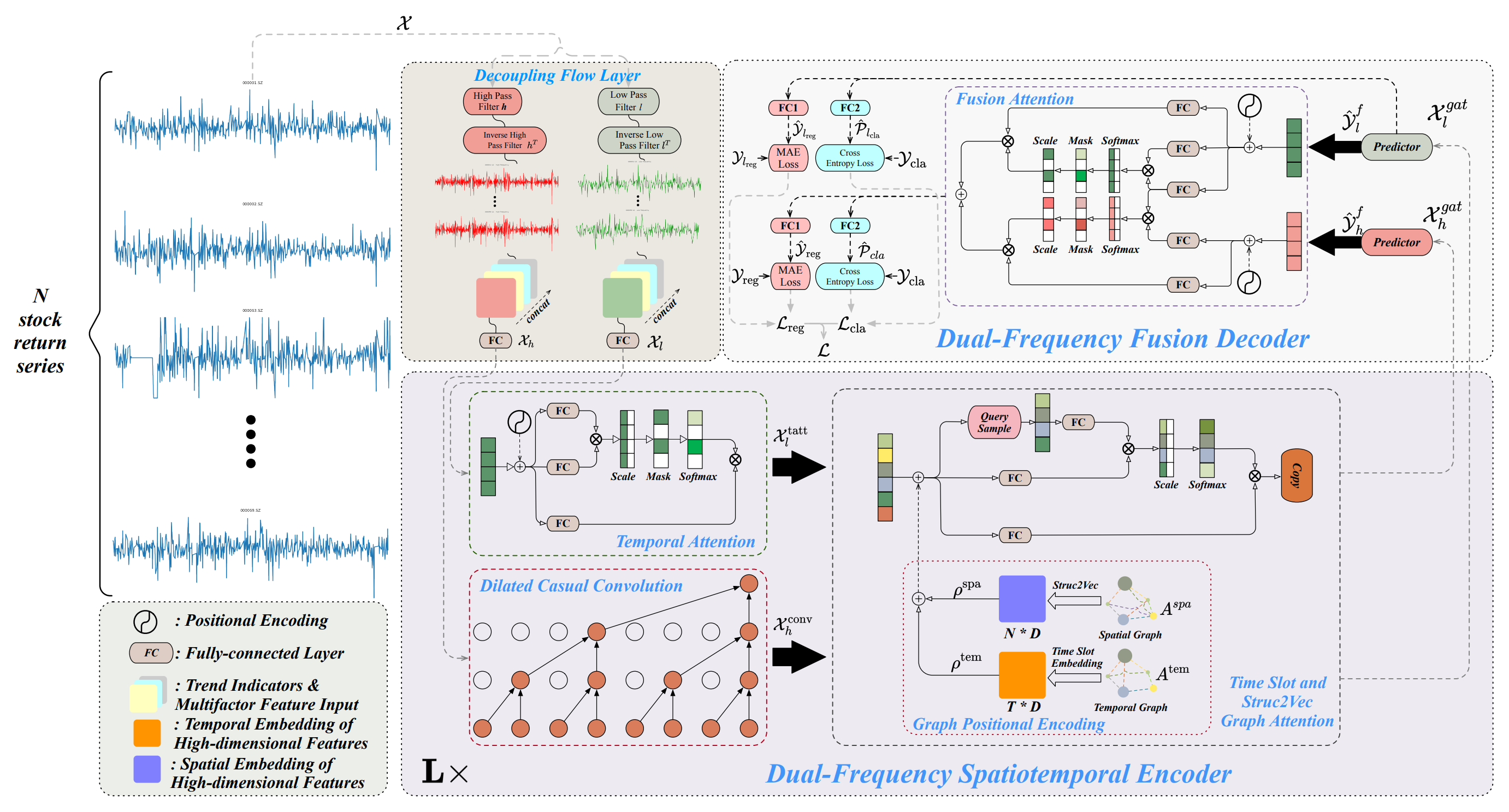
The framework is built around three core blocks. In the time series decomposition module, the analyzed data are divided into high- and low-frequency components. The low-frequency components represent global trends and support long-term pattern analysis. The high-frequency components capture short-term fluctuations, including bursts of activity and anomalies. Detailed data decomposition enhances processing quality and facilitates the extraction of key features, which plays a critically important role when working with financial time series.

After decomposition, the data are processed by a dual-frequency spatio-temporal encoder. This module combines several submodules and is designed to analyze the extracted frequency components as well as their interdependencies. Low-frequency signals are processed by a temporal attention mechanism focused on long-term trends and their evolution. High-frequency data, in turn, pass through extended causal convolutional layers that identify subtle variations and their dynamics. The processed signals are then integrated through graph attention modules that capture spatio-temporal dependencies, reflecting relationships among various assets and time intervals. This process yields multi-level graph representations, which are transformed into multidimensional embeddings. These embeddings are merged using addition and graph attention mechanisms, forming a comprehensive representation of the data for subsequent analysis.

A key stage of processing is the dual-frequency fusion decoder, which plays a crucial role in generating predictive outcomes. The decoder integrates predictors using a Fusion Attention mechanism, enabling the aggregation of low- and high-frequency data into a unified latent representation. This representation reflects temporal patterns across multiple scales, providing a comprehensive approach to data analysis. At this stage, the model generates hidden representations that are subsequently processed by specialized fully connected layers. These layers enable the model to perform multiple tasks simultaneously: forecasting asset returns, estimating trend change probabilities, and identifying other key characteristics of time series. The multitask processing approach makes the model flexible and adaptable to diverse market conditions—an especially important feature in the context of high financial market volatility.

An author-provided visualization of the Multitask-Stockformer framework is shown below.

Implementation of the Multitask-Stockformer Framework

We continue our work on implementing the approaches proposed by the authors of the Multitask-Stockformer framework in MQL5. This involves the practical implementation of key system components aimed at optimizing time series analysis.

One of the fundamental elements of the framework is the time series decomposition module, implemented within the CNeuronDecouplingFlow class. This component separates the input data into high- and low-frequency components, forming the foundation for subsequent analysis. The primary objective of this module is to extract the key structural characteristics of time series, considering their specificity and potential market trends. In the previous article, we examined the architectural and algorithmic solutions underlying the design of the CNeuronDecouplingFlow class.

The next stage of data processing involves analysis through a dual-frequency spatio-temporal encoder. As mentioned earlier, the framework authors proposed a complex encoder architecture that includes two independent data streams, each with its own structural design.

Low-frequency components are analyzed using a temporal attention mechanism based on the Self-Attention architecture. This approach provides powerful capabilities for identifying long-term dependencies and predicting global market trends. The use of Self-Attention ensures a deep understanding of complex data structures, minimizing the risk of overlooking significant interdependencies. In our current implementation, we decided to use one of the existing attention modules from our library, employing the Self-Attention mechanism.

High-frequency time series components are processed through an enhanced causal convolution module, implemented in the CNeuronDilatedCasualConv class. The improved algorithms effectively detect local anomalies and bursts of activity. This component plays a key role in analyzing short-term market dynamics, particularly during periods of high volatility. Integrating this module into the overall framework architecture increases adaptability and performance. The architectural choices and local modifications of the original framework that we used in designing CNeuronDilatedCasualConv were discussed in the previous article.

After the preliminary processing of the high- and low-frequency components of the analyzed signal, the data is routed into separate branches of the graph attention slot. This module is based on the creation of two specialized graphs. The first graph models temporal dependencies, emphasizing their sequential structure. It plays an important role in identifying trends, cyclicality, and other temporal characteristics. The second graph is based on the correlation matrix of financial asset prices, providing deep integration of information about asset interdependencies. This enables the model to account for the influence of one asset on another, which is especially important for financial modeling and forecasting. Together, these graphs form a multi-level structure that enhances the accuracy of data analysis and interpretation.

To convert graph information into analytically useful representations, the Struct2Vec algorithm is employed. This algorithm translates the topological properties of graphs into compact vector embeddings, which are further optimized using trainable fully connected layers. Such embeddings allow for the efficient integration of local and global data features, improving time series analysis quality. The processed data is then passed to graph attention branches, where it undergoes further examination using attention mechanisms. This stage enables the detection of both short-term and long-term dependencies.

The authors of the Multitask-Stockformer framework proposed a rather complex architecture for the graph attention slot. Its implementation would require substantial computational resources and meticulous data preparation. In preparing the model for this study, we introduced several simplifications aimed at improving the model's practical usability while maintaining high performance. The first simplification involved excluding temporal information about the analyzed environmental state. This decision was based on the assumption that temporal information, while useful, does not critically affect the overall efficiency of our model at this stage. In the original framework, the output represented a constructed stock portfolio, whereas in our implementation, the main objective is to create a latent representation of the environment. This representation is used by the Actor model to make trading decisions, supplemented by account state and timestamp data, providing contextual awareness. Thus, we merely shift the point at which temporal information is transferred to the model.

However, the simplification applied to the temporal dependency graph cannot be used for the asset correlation graph, as this would result in the loss of critical information. Instead, we propose an alternative solution by replacing the original structure with a trainable positional encoding layer. This approach effectively trains embeddings while minimizing computational complexity and preserving essential inter-asset relationships, which the model learns autonomously during training. This improvement provides a more flexible architecture capable of adapting to diverse market conditions.

Additionally, we made another step forward by replacing the graph attention slots with Node-Adaptive Feature Smoothing (NAFS) modules. A key advantage of this method is the absence of trainable parameters in NAFS modules, which not only reduces computational complexity but also simplifies model configuration and training.

When using NAFS, the embedding construction process becomes more flexible and robust, as the smoothing method adapts to the graph's topology and node characteristics. This is especially important for tasks where the data structure may be heterogeneous or dynamically changing. Consequently, NAFS enables the creation of high-quality data representations that simultaneously account for both local and global graph relationships.

Aggregation of the two information streams is performed in a dual-frequency decoder, which integrates different aspects of the data to create a foundation for multidimensional analysis. This allows for a more comprehensive representation of signal dynamics. The dual-frequency decoder is based on the Fusion Attention mechanism, which combines two parallel attention modules. The first module, based on Self-Attention, specializes in deep processing of low-frequency components, identifying key long-term dependencies, stable trends, and global patterns. This module makes it possible to capture fundamental time series characteristics that play a crucial role in forecasting. The second module employs Cross-Attention to integrate high-frequency information, enriching the analysis with short-term and fine-grained components. Such integration significantly enhances low-frequency data with detail? particularly important for accounting for subtle but meaningful fluctuations.

Both attention modules operate synchronously, ensuring the creation of coherent and complementary data representations. Their results are merged through summation and subsequently processed by fully connected layers (MLP). This approach allows for the simultaneous consideration of global and local signal features, capturing a broad range of relationships and influences.

The proposed Fusion Attention architecture can be easily implemented using existing Cross- and Self-Attention modules. Moreover, its implementation does not require significant changes to the basic algorithms.

Thus, we can conclude that we now have all the key modules for creating a comprehensive architecture of the Multitask-Stockformer framework. This produces the basis for moving on to the next development step: the formation of a high-level object that will unite all of the specified modules into a single, functionally complete algorithm. The main purpose of this step is not only to integrate the components, but also to ensure their synchronous operation, taking into account the characteristics of each module. Below is the structure of the new CNeuronMulttaskStockformer object.

class CNeuronMultitaskStockformer   :  public CNeuronBaseOCL
  {
protected:
   CNeuronDecouplingFlow      cDecouplingFlow;
   CNeuronBaseOCL             cLowFreqSignal;
   CNeuronBaseOCL             cHighFreqSignal;
   CNeuronRMAT                cTemporalAttention;
   CNeuronDilatedCasualConv   cDilatedCasualConvolution;
   CNeuronLearnabledPE        cLowFreqPE;
   CNeuronLearnabledPE        cHighFreqPE;
   CNeuronNAFS                cLowFreqGraphAttention;
   CNeuronNAFS                cHighFreqGraphAttention;
   CNeuronDMHAttention        cLowFreqFusionDecoder;
   CNeuronCrossDMHAttention   cLowHighFreqFusionDecoder;
   CNeuronBaseOCL             cLowHigh;
   CNeuronConvOCL             cProjection;
   //---
   virtual bool      feedForward(CNeuronBaseOCL *NeuronOCL) override;
   virtual bool      calcInputGradients(CNeuronBaseOCL *prevLayer) override;
   virtual bool      updateInputWeights(CNeuronBaseOCL *NeuronOCL) override;

public:
                     CNeuronMultitaskStockformer(void) {};
                    ~CNeuronMultitaskStockformer(void) {};
   virtual bool      Init(uint numOutputs, uint myIndex, COpenCLMy *open_cl,
                          uint window, uint window_key, uint units_count,
                          uint heads, uint layers, uint neurons_out, uint filters,
                          ENUM_OPTIMIZATION optimization_type, uint batch);
   //---
   virtual int       Type(void) override   const   {  return defNeuronMultitaskStockformer; }
   //---
   virtual bool      Save(int const file_handle) override;
   virtual bool      Load(int const file_handle) override;
   //---
   virtual bool      WeightsUpdate(CNeuronBaseOCL *source, float tau) override;
   virtual void      SetOpenCL(COpenCLMy *obj) override;
  };

The presented structure includes numerous internal objects that directly correspond to the modules of the Multitask-Stockformer framework described above. These components are organized to ensure a high degree of functional integration and flexibility in implementation. We will analyze in detail the algorithms governing their interaction, as well as the data flow during the implementation of the integration object methods.

All internal objects are declared as static, allowing us to keep the class constructor and destructor empty. Initialization of all newly declared and inherited objects is performed within the Init method.

bool CNeuronMultitaskStockformer::Init(uint numOutputs, uint myIndex, COpenCLMy *open_cl,
                                       uint window, uint window_key, uint units_count,
                                       uint heads, uint layers, uint neurons_out, uint filters,
                                       ENUM_OPTIMIZATION optimization_type, uint batch)
  {
   if(!CNeuronBaseOCL::Init(numOutputs, myIndex, open_cl, neurons_out, optimization_type, batch))
      return false;

Among the parameters of this method, in addition to familiar constants, there is a new parameter: neurons_out. It specifies the size of the latent representation vector of the analyzed environmental state, which the user expects to obtain as the output of this Multitask-Stockformer block. This vector is passed to the corresponding method of the parent class, which initializes the core interfaces for data exchange with external neural layers within the model.

After successfully executing the parent class method, we move on to initializing the internal objects. This process follows the order of object usage during the feed-forward pass. As previously mentioned, the input data is first separated into high- and low-frequency components by the CNeuronDecouplingFlow signal decomposition module.

   uint index = 0;
   uint wave_window = MathMin(24, units_count);
   if(!cDecouplingFlow.Init(0, index, OpenCL, wave_window, 2, units_count, filters, window, optimization, iBatch))
      return false;
   cDecouplingFlow.SetActivationFunction(None);

Note that in the external parameters of the integration object's initialization method, we do not specify the size and step of the discrete wavelet transform window. These parameters are set to fixed values directly in the method. For the experiments described in this article, we focus on historical H1 timeframe data. Accordingly, we limit the wavelet transform window size to one day, corresponding to 24 steps of the analyzed sequence, and add a check to prevent exceeding the length of the multimodal time series. The window step is set to 2, effectively skipping one element of the sequence.

The output of the decomposition module is a unified tensor containing both high- and low-frequency components. For processing in the dual-frequency spatio-temporal encoder, two parallel streams are provided, with each component analyzed separately. To implement this approach, we split the data into individual objects. This will provide convenience and flexibility for subsequent processing.

//--- Dual-Frequency Spatiotemporal Encoder
   uint wave_units_out = cDecouplingFlow.GetUnits();
   index++;
   if(!cLowFreqSignal.Init(0, index, OpenCL, cDecouplingFlow.Neurons() / 2, optimization, iBatch))
      return false;
   cLowFreqSignal.SetActivationFunction(None);
   index++;
   if(!cHighFreqSignal.Init(0, index, OpenCL, cDecouplingFlow.Neurons() / 2, optimization, iBatch))
      return false;
   cHighFreqSignal.SetActivationFunction(None);
   index++;

The low-frequency component is processed in the temporal attention module, based on the Self-Attention mechanism. In the original Multitask-Stockformer framework, positional encoding is proposed to enhance sequence processing. However, we use an attention module with relative positional encoding, which inherently determines the relative positions of sequence elements. This eliminates the need for additional positional encoding, simplifying the architecture while improving efficiency.

   if(!cTemporalAttention.Init(0, index, OpenCL, filters, window_key, wave_units_out * window, heads, layers,
                                                                                       optimization, iBatch))
      return false;
   cTemporalAttention.SetActivationFunction(None);
   index++;

It is important to note that the dimension of the vector describing a single sequence element corresponds to the number of filters used in the wavelet transform. While the sequence length covers all univariate time series. This approach enables the study of trend interdependencies across the entire multimodal sequence, rather than analyzing its components in isolation.

High-frequency dependencies are analyzed in the enhanced causal convolution module. Here we use a minimal convolution window of 2 elements with the same step. Analysis is performed within unit sequences, allowing detailed investigation of local dependencies.

   if(!cDilatedCasualConvolution.Init(0, index, OpenCL, 2, 2, filters, wave_units_out, window, layers,
                                                                                 optimization, iBatch))
      return false;
   index++;

Positional encoding is then added to both components.

   if(!cLowFreqPE.Init(0, index, OpenCL, cTemporalAttention.Neurons(), optimization, iBatch))
      return false;
   index++;
   if(!cHighFreqPE.Init(0, index, OpenCL, cDilatedCasualConvolution.Neurons(), optimization, iBatch))
      return false;
   index++;

Each component receives a separate trainable positional encoding layer. This approach enables facilitating deeper analysis of high- and low-frequency structures independently.

Upon completing the dual-frequency encoder, we initialize Node-Adaptive Feature Smoothing (NAFS) modules, applied separately to high- and low-frequency components. Both modules share parameters except for sequence length. The high-frequency sequence is expected to be shorter due to the nature of the enhanced causal convolution module.

   if(!cLowFreqGraphAttention.Init(0, index, OpenCL, filters, 3, wave_units_out * window, optimization, iBatch))
      return false;
   index++;
   if(!cHighFreqGraphAttention.Init(0, index, OpenCL, filters, 3, cDilatedCasualConvolution.Neurons()/filters,
                                                                                          optimization, iBatch))
      return false;
   index++;

Next, we initialize the data flow fusion decoder objects. Here we initialize two attention blocks: Self-Attention for low-frequency components and Cross-Attention for integrating high-frequency components.

//--- Dual-Frequency Fusion Decoder
   if(!cLowFreqFusionDecoder.Init(0, index, OpenCL, filters, window_key, wave_units_out * window, heads,
                                                                           layers, optimization, iBatch))
      return false;
   index++;
   if(!cLowHighFreqFusionDecoder.Init(0, index, OpenCL, filters, window_key, wave_units_out * window, filters,
                             cDilatedCasualConvolution.Neurons()/filters, heads, layers, optimization, iBatch))
      return false;
   index++;

The attention block outputs are summed. And a base neural layer object is created to store the results.

   if(!cLowHigh.Init(0, index, OpenCL, cLowFreqFusionDecoder.Neurons(), optimization, iBatch))
      return false;
   CBufferFloat *grad = cLowFreqFusionDecoder.getGradient();
   if(!grad ||
      !cLowHigh.SetGradient(grad, true) ||
      !cLowHighFreqFusionDecoder.SetGradient(grad, true))
      return false;
   index++;

To reduce unnecessary data copying, pointers to the gradient buffers of the last three objects are synchronized. This approach reduces memory usage and improves training efficiency.

Finally, we initialize the MLP objects for generating the latent representation of the environmental state. Here we use a convolutional layer for dimensionality reduction and a fully connected layer to produce the target representation size.

The fully connected layer is inherited from the parent class, allowing us to initialize only the convolutional layer with the required output connections. To implement the functionality of the fully connected layer, we will use the inherited capabilities of the parent class.

   if(!cProjection.Init(Neurons(), index, OpenCL, filters, filters, 3, wave_units_out, window, optimization, iBatch))
      return false;
//---
   return true;
  }

After initializing all internal objects, the Init method concludes, returning a logical success status to the calling program.

We then construct the feedForward algorithm for the integration object.

bool CNeuronMultitaskStockformer::feedForward(CNeuronBaseOCL *NeuronOCL)
  {
//--- Decoupling Flow
   if(!cDecouplingFlow.FeedForward(NeuronOCL))
      return false;

The method receives a pointer to the input data object, which is passed to the decomposition module.

The resulting tensor is split between the two streams for independent analysis.

   if(!DeConcat(cLowFreqSignal.getOutput(), cHighFreqSignal.getOutput(), cDecouplingFlow.getOutput(),
                                          cDecouplingFlow.GetFilters(), cDecouplingFlow.GetFilters(), 
                                          cDecouplingFlow.GetUnits()*cDecouplingFlow.GetVariables()))
      return false;

The low-frequency component proceeds through the temporal attention module. Then it receives positional encoding, and enters the graph representation module.

//--- Dual-Frequency Spatiotemporal Encoder
//--- Low Frequency Encoder
   if(!cTemporalAttention.FeedForward(cLowFreqSignal.AsObject()))
      return false;
   if(!cLowFreqPE.FeedForward(cTemporalAttention.AsObject()))
      return false;
   if(!cLowFreqGraphAttention.FeedForward(cLowFreqPE.AsObject()))
      return false;

The high-frequency component follows its stream starting from the enhanced causal convolution module.

//--- High Frequency Encoder
   if(!cDilatedCasualConvolution.FeedForward(cHighFreqSignal.AsObject()))
      return false;
   if(!cHighFreqPE.FeedForward(cDilatedCasualConvolution.AsObject()))
      return false;
   if(!cHighFreqGraphAttention.FeedForward(cHighFreqPE.AsObject()))
      return false;

Outputs from both streams are passed to the dual-frequency fusion decoder. Here the data is first processed by two attention modules. The outputs are summed and normalized.

//--- Dual-Frequency Fusion Decoder
   if(!cLowFreqFusionDecoder.FeedForward(cLowFreqGraphAttention.AsObject()))
      return false;
   if(!cLowHighFreqFusionDecoder.FeedForward(cLowFreqGraphAttention.AsObject(), cHighFreqGraphAttention.getOutput()))
      return false;
   if(!SumAndNormilize(cLowFreqFusionDecoder.getOutput(), cLowHighFreqFusionDecoder.getOutput(), cLowHigh.getOutput(),
                                                                 cLowFreqFusionDecoder.GetWindow(), true, 0, 0, 0, 1))
      return false;

Next, the data is compressed via a convolutional projection layer.

   if(!cProjection.FeedForward(cLowHigh.AsObject()))
      return false;
//---
   return CNeuronBaseOCL::feedForward(cProjection.AsObject());
  }

The result is then sent to the parent class method to generate the final representation of the analyzed state of the environment.

The next step is to implement backpropagation processes, which play a key role in training the model. Backpropagation is organized in calcInputGradients, following the feed-forward pass in reverse.

bool CNeuronMultitaskStockformer::calcInputGradients(CNeuronBaseOCL *prevLayer)
  {
   if(!prevLayer)
      return false;

The parameters of this method include a pointer to the source data object; into its buffer we need to pass the error gradient, distributed in accordance with the influence of the input data on the final model output. And in the body of the method, we check the relevance of the received pointer. Otherwise, data transfer becomes impossible.

Gradients are first applied to the convolutional projection layer using the parent class functionality. Then they are propagated to the summation layer of the dual-frequency decoder.

   if(!CNeuronBaseOCL::calcInputGradients(cProjection.AsObject()))
      return false;
   if(!cLowHigh.calcHiddenGradients(cProjection.AsObject()))
      return false;

During the initialization of the integration object, we implemented the substitution of pointers to the error gradient buffers used by the decoder attention modules and the output summation layer. This ensures that the entire error gradient propagated to the summation layer is fully passed to the corresponding attention modules. So, we can move directly to gradient propagation through the decoder's attention modules.

However, it should be noted that the low-frequency component data is simultaneously used in both attention blocks. Therefore, we need to obtain the error gradient from two information streams. We first perform the error gradient distribution operations through the Self-Attention module.

//--- Dual-Frequency Fusion Decoder
   if(!cLowFreqGraphAttention.calcHiddenGradients(cLowFreqFusionDecoder.AsObject()))
      return false;

Then we perform a temporary substitution of the pointer to the Self-Attention module error gradient buffer with a free buffer of a similar size and perform operations of the Cross-Attention error gradient propagation operations.

   CBufferFloat *grad = cLowFreqGraphAttention.getGradient();
   if(!cLowFreqGraphAttention.SetGradient(cLowFreqGraphAttention.getPrevOutput(), false) ||
      !cLowFreqGraphAttention.calcHiddenGradients(cLowHighFreqFusionDecoder.AsObject(),
            cHighFreqGraphAttention.getOutput(),
            cHighFreqGraphAttention.getGradient(),
            (ENUM_ACTIVATION)cHighFreqGraphAttention.Activation()) ||
      !SumAndNormilize(grad, cLowFreqGraphAttention.getGradient(), grad, 1, false, 0, 0, 0, 1) ||
      !cLowFreqGraphAttention.SetGradient(grad, false))
      return false;

Then we sum the data of the two information streams and return the pointers to the data buffers to their original state.

We have distributed the error gradient to high- and low-frequency components at the level of the dual-frequency spatiotemporal encoder output. Next, we sequentially distribute the gradient among the objects of two independent streams. Low-frequency:

//--- Dual-Frequency Spatiotemporal Encoder
//--- Low Frequency Encoder
   if(!cLowFreqPE.calcHiddenGradients(cLowFreqGraphAttention.AsObject()))
      return false;
   if(!cTemporalAttention.calcHiddenGradients(cLowFreqPE.AsObject()))
      return false;
   if(!cLowFreqSignal.calcHiddenGradients(cTemporalAttention.AsObject()))
      return false;

Then high-frequency:

//--- High Frequency Encoder
   if(!cHighFreqPE.calcHiddenGradients(cHighFreqGraphAttention.AsObject()))
      return false;
   if(!cDilatedCasualConvolution.calcHiddenGradients(cHighFreqPE.AsObject()))
      return false;
   if(!cHighFreqSignal.calcHiddenGradients(cDilatedCasualConvolution.AsObject()))
      return false;

Gradients from both streams are concatenated into a single tensor:

//--- Decoupling Flow
   if(!Concat(cLowFreqSignal.getGradient(), cHighFreqSignal.getGradient(),
              cDecouplingFlow.getGradient(), cDecouplingFlow.GetFilters(),
              cDecouplingFlow.GetFilters(), cDecouplingFlow.GetUnits()*cDecouplingFlow.GetVariables()))
      return false;
   if(!prevLayer.calcHiddenGradients(cDecouplingFlow.AsObject()))
      return false;
//---
   return true;
  }

And then they are propagated back through the decomposition module to the input data. The method concludes by returning the logical result of the operation to the calling program.

Parameter optimization in updateInputWeights is performed in the same order but only for objects with trainable parameters. The method is left for independent study, and the full code of the integration object and all its methods is available in the attachment.

This concludes the discussion of the Multitask-Stockformer framework implementation algorithms. The next step is integrating the realized approaches into the architecture of trainable models.

Model Architecture

The approaches of the Multitask-Stockformer framework implemented above are now applied in the environment state encoder model. Thanks to the use of the comprehensive Multitask-Stockformer implementation object, the model architecture remains quite compact - it consists of only three layers. As usual, we start with the input data and batch normalization layers.

bool CreateEncoderDescriptions(CArrayObj *&encoder)
  {
//---
   CLayerDescription *descr;
//---
   if(!encoder)
     {
      encoder = new CArrayObj();
      if(!encoder)
         return false;
     }
//--- Encoder
   encoder.Clear();
//--- Input layer
   if(!(descr = new CLayerDescription()))
      return false;
   descr.type = defNeuronBaseOCL;
   int prev_count = descr.count = (HistoryBars * BarDescr);
   descr.activation = None;
   descr.optimization = ADAM;
   if(!encoder.Add(descr))
     {
      delete descr;
      return false;
     }
//--- layer 1
   if(!(descr = new CLayerDescription()))
      return false;
   descr.type = defNeuronBatchNormOCL;
   descr.count = prev_count;
   descr.batch = 1e4;
   descr.activation = None;
   descr.optimization = ADAM;
   if(!encoder.Add(descr))
     {
      delete descr;
      return false;
     }

These layers perform preliminary processing of the raw input data received from the environment. They are followed by a new layer implementing the Multitask-Stockformer framework approaches.

//--- layer 2
   if(!(descr = new CLayerDescription()))
      return false;
   descr.type = defNeuronMultitaskStockformer;
//--- Windows
     {
      int temp[] = {BarDescr, 10, LatentCount}; //Window, Filters, Output
      if(ArrayCopy(descr.windows, temp) < int(temp.Size()))
         return false;
     }
   descr.count = HistoryBars;
   descr.window_out = 32;
   descr.step = 4;                              // Heads
   descr.layers = 3;
   descr.batch = 1e4;
   descr.activation = None;
   descr.optimization = ADAM;
   if(!encoder.Add(descr))
     {
      delete descr;
      return false;
     }
//---
   return true;
  }

In our experiment, 10 wavelet filters were used. Each attention module employed 4 heads and contained 3 internal layers.

The outputs of the environment state encoder are used by two models: the Actor, which makes trading decisions, and the Critic, which evaluates the actions generated by the Actor. The architectures of these models were adopted from our previous studies, along with the environment interaction and training programs. The complete model architectures and the full program code used in this article are available in the attachment. We now proceed to the final stage — testing the effectiveness of the implemented solutions on real historical data.

Testing

Over the course of two articles, we performed extensive work implementing the approaches proposed by the authors of the Multitask-Stockformer framework using MQL5. It is now time for the most exciting stage — testing the effectiveness of the implemented solutions on real historical data.

It is important to clarify that we are evaluating the implemented approaches rather than the original Multitask-Stockformer framework, as several modifications were introduced during implementation.

During testing, the models were trained on EURUSD historical data for the entire year of 2023, with the H1 timeframe. All analyzed indicators were used with their default parameter settings.

For the initial training phase, we used a dataset collected in previous studies. This dataset was periodically updated to adapt to the evolving Actor policy. After several training and dataset update cycles, the resulting policy demonstrated profitability on both the training and test sets.

Testing of the trained policy was conducted on historical data for January 2024, with all other parameters unchanged. The results are presented below.

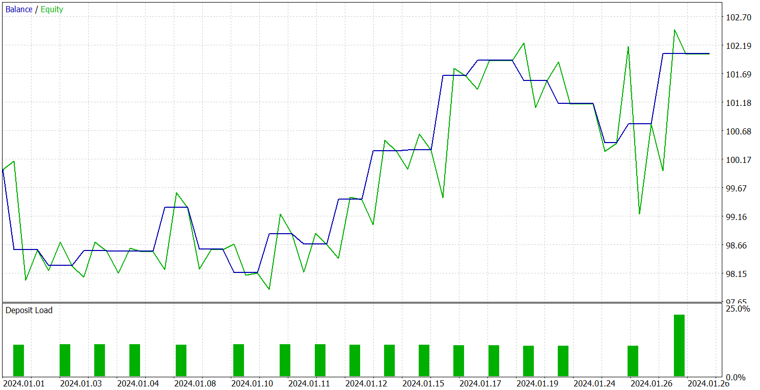
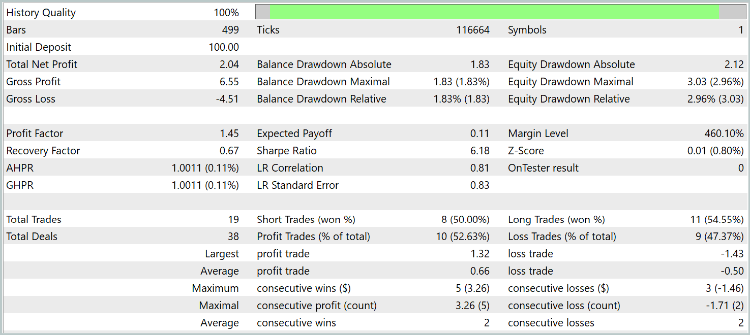
During the testing period, the model executed 19 trades, 10 of which closed with a profit. This is slightly above 50%. However, due to the higher average profit per winning trade compared to losing positions, the model ended the testing period with an overall profit, achieving a profit factor of 1.45.

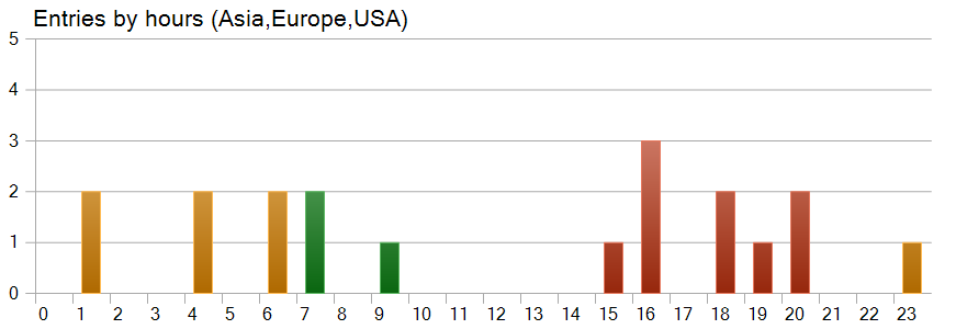
An interesting observation comes from the trade timing chart. Nearly half of the trades were opened during the U.S. trading session, while the model executed almost no trades during the periods of highest volatility.

Conclusion

We explored the Multitask-Stockformer framework - an innovative stock selection model that combines discrete wavelet transformation with multitask Self-Attention modules. This comprehensive approach enables the identification of temporal and frequency features in market data, allowing accurate modeling of complex interactions between analyzed factors.

In the practical section, we developed our own implementation of the framework approaches in MQL5. We integrated the approaches into the model architectures, and trained these models on real historical data. The trained models were then tested in the MetaTrader 5 Strategy Tester. The results of our experiments demonstrate the potential of the implemented solutions. However, before applying them in real trading, the models should be trained on a more representative dataset and subjected to comprehensive testing.

References

• Stockformer: A Price-Volume Factor Stock Selection Model Based on Wavelet Transform and Multi-Task Self-Attention Networks
• Other articles from this series

Programs used in the article

#	Name	Type	Description
1	Research.mq5	Expert Advisor	Expert Advisor for collecting samples
2	ResearchRealORL.mq5	Expert Advisor	Expert Advisor for collecting samples using the Real-ORL method
3	Study.mq5	Expert Advisor	Model training EA
4	Test.mq5	Expert Advisor	Model Testing Expert Advisor
5	Trajectory.mqh	Class library	System state and model architecture description structure
6	NeuroNet.mqh	Class library	A library of classes for creating a neural network
7	NeuroNet.cl	Code Base	Библиотека кода OpenCL-программы