Blood inheritance optimization (BIO)

Contents

1. Introduction
2. Implementation of the algorithm
3. Test results

Introduction

One day, as I was watching a nurse collect blood specimens from patients in the lab, a sudden thought struck me. Blood groups, this ancient system of inheritance, passed down from generation to generation according to strict genetic laws, suddenly appeared before me in a completely new light. What if these natural properties of inheritance could be exploited in the field of optimization algorithms?

Each of us carries in our veins a unique combination inherited from our parents. Just as blood types determine compatibility during transfusions, they could determine how parameters are transferred and mutated during the optimization. I liked this idea and decided to come back to it when I had time to do research. After conducting experiments, the Blood Inheritance Optimization (BIO) algorithm was born – a method that uses the natural laws of blood group inheritance as a metaphor for managing the evolution of decisions. In the algorithm, the four blood types evolved into four different strategies for mutation of parameters, and the laws of inheritance determined how offspring acquire and modify the characteristics of their parents.

As in nature, a child's blood type is not a simple average of the parents' blood types, but is subject to genetic laws. In BIO, the parameters of new solutions are formed through a system of inheritance and mutations. Each blood type brings its own unique approach to exploring the solution space: from conservatively preserving the best values found, to radical mutations that open up new promising areas and directions for further research into the solution space.

In this article, I would like to share the principles of the BIO algorithm, which combines biological inspiration with algorithmic rigor, and provide test results on functions we are already familiar with. So, let us do that.

Implementation of the algorithm

First, let's get acquainted with the table of inheritance of the blood type of the offspring from the parents. As you can see, the inheritance of blood group is not uniform. There are interesting statistics on the distribution of blood types among the population in the world. The most common is the first group (O) — about 40% of the planet's population are its carriers. It is followed by the second group (A), which is possessed by approximately 30% of people. The third group (B) occurs in 20% of the population, and the fourth one (AB)  is the rarest - only about 10% of people carry it.

While studying the mechanisms of inheritance, I learned that the first blood group is recessive in relation to all the others. This means that people with blood type 1 can only pass on blood type 1 to their children. At the same time, the second and third groups demonstrate co-dominance with respect to each other, which leads to the emergence of the fourth group when they are combined. From an evolutionary point of view, the fourth blood group is the youngest.

I was particularly interested in some of the unique properties of different blood types. For example, blood type O is considered a "universal donor" because it can be transfused into people with any blood type. The fourth group, on the contrary, makes its carriers "universal recipients" – they can accept blood of any type. 

All these features of the blood group system inspired me to create corresponding mechanisms in my algorithm. Since the first blood group is the basic and most common, it corresponds to the strategy of preserving the best solution found in the algorithm. The blood group inheritance table, showing all possible combinations of parental blood groups and the potential blood groups of their children, forms the basis for determining the "blood group" of a new solution based on the "blood groups" of parental solutions, which directly influences the way parameters are mutated in the BIO algorithm.

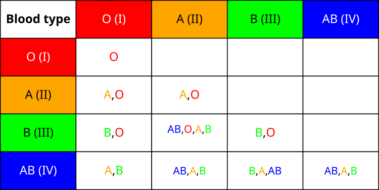
Figure 1. Blood group inheritance table 

The BIO algorithm is based on a fairly simple idea: each solution in the population (parent individuals) has its own "blood group" (from 1 to 4), which is determined by its ordinal number in the population. When we create a new generation of solutions, we select two "parents" from the current population. The probability of choice is not linear, but quadratic — this means that the best decisions have a significantly higher chance of becoming parents.

Now the most interesting part begins. Based on the parents' blood types, using a special inheritance matrix (it is written in the code in the Init method), we determine the possible blood types for the "child" - the new solution. Then, for each parameter of this new solution, if the first blood group is found, we take the value from the best solution found. I did this by analogy with the first blood group as a universal donor. If the second group is selected, we take the value from one of the parents and apply the power distribution to it. This creates a tendency to explore the edges of the parameter range. For the third group, we also take a value from one of the parents, but move it towards the best solution by a random amount. And with the fourth group, we take the parent value and reflect it relative to the range boundaries, a kind of inversion, which allows us to explore new search areas.

After creating a new generation, we check whether any better solutions than the current global solution have emerged and save the best individuals for the next iteration. So, using the analogy of blood group inheritance, my algorithm explores the solution space by combining different parameter mutation strategies. Below is the pseudocode of the algorithm.

Initialization:

1. Create a population of agents of popSize (default 50)
2. Create a blood group inheritance matrix that determines the possible blood groups of children based on the blood groups of the parents (1,2,3,4)
3. Initialization of ranges for parameters (min., max., step values)

Main loop:

1. If this is the first iteration (revision = false):
   • Randomly initialize the positions of all agents within the parameter ranges
   • Set the revision flag to 'true'
2. For each agent in the population:
   • Select parental agents (father and mother) using a quadratic probability distribution
   • Determine the blood types of both parents using the function: bloodType = 1 + (population_position % 4)
   • For each parameter of the child solution:
     • Obtain the child's probable blood type from the inheritance matrix based on the parents' blood types
     • If the child has blood type 1:
       • Use the best known solution for this parameter.
     • Otherwise:
       • Randomly select a parameter value from either the father or the mother
       • Apply mutation based on child's blood type:
         • Type 2: Apply a power-law distribution with exponent 20
         • Type 3: Move the parameter value towards the best solution with a random factor
         • Type 4: Mirror parameter value across the entire parameter range
     • Ensure that the parameter remains within the acceptable range and step

Revision phase:

1. Update the global best solution if any agent has better fitness
2. Copy the current population to the second half of the expanded population array
3. Sort the extended population by fitness
4. Preserve the best agents for the next generation

Let's start writing the algorithm code. The C_AO_BIO class derived from C_AO implements the BIO algorithm and assumes the use of a data structure to represent individuals (agents) in a population, as well as their control.

C_AO_BIO ()  — constructor, which initializes the external BIO parameters: the popSize population size is set to 50, the size of the 'params' parameter array is set to one element representing popSize.
SetParams ()  — the method allows setting class parameters, in this case setting the popSize population size from the parameters array.
Init () — the method initializes the algorithm by accepting the minimum and maximum values of the parameters, the step of change, and the number of epochs.
Moving () and Revision () — methods are responsible for the movement (evolution) of agents in the population and their revision (performance assessment and selection of the best ones).
S_Papa and S_Mama:

• S_Papa is a structure containing an array of blood types (bTypes).
• S_Mama contains the array of four S_Papa objects, which suggests the presence of "parents" for further genetic mixing.

This method of representation in the form of structures will allow us to directly obtain the probable blood group of the offspring from the parents, by specifying the blood group of the parents, so "ma [1].pa [2].bTypes", where 1 and 2 are the blood groups of the mother and father, respectively.

The GetBloodType ()method ) returns the blood type for a given agent, while GetBloodMutation () implements the mechanism of gene mutation depending on the blood type.

//——————————————————————————————————————————————————————————————————————————————
class C_AO_BIO : public C_AO
{
  public: //--------------------------------------------------------------------
  C_AO_BIO ()
  {
    ao_name = "BIO";
    ao_desc = "Blood Inheritance Optimization";
    ao_link = "https://www.mql5.com/en/articles/17246";

    popSize = 50; // population size

    ArrayResize (params, 1);
    params [0].name = "popSize"; params [0].val = popSize;
  }

  void SetParams ()
  {
    popSize = (int)params [0].val;
  }

  bool Init (const double &rangeMinP  [],  // minimum values
             const double &rangeMaxP  [],  // maximum values
             const double &rangeStepP [],  // step change
             const int     epochsP = 0);   // number of epochs

  void Moving   ();
  void Revision ();

  private: //-------------------------------------------------------------------
  struct S_Papa
  {
      int bTypes [];
  };
  struct S_Mama
  {
      S_Papa pa [4];
  };
  S_Mama ma [4];

  S_AO_Agent p [];

  int  GetBloodType     (int ind);
  void GetBloodMutation (double &gene, int indGene, int bloodType);
};
//——————————————————————————————————————————————————————————————————————————————

The Init method initializes an instance of the C_AO_BIO class and prepares it for work by setting up the agent population and their characteristics. Let's look at the implementation of this method.

Calling the StandardInit method — the first string checks the result of calling the method, which checks/initializes the basic parameters required for the algorithm to work.

Initializing the agent array:

• Resizes the "p" agent array to twice the given population size (popSize).
• In the for loop, the Init method is called for each agent, initializing the agent using the coordinate parameters.

Initialization of blood types:

• Next, the method specifies the size of the arrays of blood types (bTypes) for the S_Mama and S_Papa structures.
• For different combinations (for example, ma [0].pa [0], ma [1].pa [2] etc.), different blood types are set according to a special inheritance matrix, and the size of the arrays is specified via ArrayResize.

So, the Init method in the C_AO_BIO class performs the important task of preparing the object for the execution of the optimization algorithm: it creates a population of agents, sets up their initial parameters, and defines the association rules for blood types (inheritance). This allows one to instantly obtain the probable blood type of the offspring, as well as use the parameters of their "blood" for further evolution within the algorithm.

//——————————————————————————————————————————————————————————————————————————————
bool C_AO_BIO::Init (const double &rangeMinP  [],
                     const double &rangeMaxP  [],
                     const double &rangeStepP [],
                     const int     epochsP = 0)
{
  if (!StandardInit (rangeMinP, rangeMaxP, rangeStepP)) return false;

  //----------------------------------------------------------------------------
  ArrayResize (p, popSize * 2);
  for (int i = 0; i < popSize * 2; i++) p [i].Init (coords);

  //1-1
  ArrayResize (ma [0].pa [0].bTypes, 1);

  ma [0].pa [0].bTypes [0] = 1;

  //2-2
  ArrayResize (ma [1].pa [1].bTypes, 2);

  ma [1].pa [1].bTypes [0] = 1;
  ma [1].pa [1].bTypes [1] = 2;

  //3-3
  ArrayResize (ma [2].pa [2].bTypes, 2);

  ma [2].pa [2].bTypes [0] = 1;
  ma [2].pa [2].bTypes [1] = 3;

  //1-2; 2-1
  ArrayResize (ma [0].pa [1].bTypes, 2);
  ArrayResize (ma [1].pa [0].bTypes, 2);

  ma [0].pa [1].bTypes [0] = 1;
  ma [0].pa [1].bTypes [1] = 2;

  ma [1].pa [0].bTypes [0] = 1;
  ma [1].pa [0].bTypes [1] = 2;

  //1-3; 3-1
  ArrayResize (ma [0].pa [2].bTypes, 2);
  ArrayResize (ma [2].pa [0].bTypes, 2);

  ma [0].pa [2].bTypes [0] = 1;
  ma [0].pa [2].bTypes [1] = 3;

  ma [2].pa [0].bTypes [0] = 1;
  ma [2].pa [0].bTypes [1] = 3;

  //1-4; 4-1
  ArrayResize (ma [0].pa [3].bTypes, 2);
  ArrayResize (ma [3].pa [0].bTypes, 2);

  ma [0].pa [3].bTypes [0] = 2;
  ma [0].pa [3].bTypes [1] = 3;

  ma [3].pa [0].bTypes [0] = 2;
  ma [3].pa [0].bTypes [1] = 3;

  //2-3; 3-2
  ArrayResize (ma [1].pa [2].bTypes, 4);
  ArrayResize (ma [2].pa [1].bTypes, 4);

  ma [1].pa [2].bTypes [0] = 1;
  ma [1].pa [2].bTypes [1] = 2;
  ma [1].pa [2].bTypes [2] = 3;
  ma [1].pa [2].bTypes [3] = 4;

  ma [2].pa [1].bTypes [0] = 1;
  ma [2].pa [1].bTypes [1] = 2;
  ma [2].pa [1].bTypes [2] = 3;
  ma [2].pa [1].bTypes [3] = 4;

  //2-4; 4-2; 3-4; 4-3; 4-4
  ArrayResize (ma [1].pa [3].bTypes, 3);
  ArrayResize (ma [3].pa [1].bTypes, 3);
  ArrayResize (ma [2].pa [3].bTypes, 3);
  ArrayResize (ma [3].pa [2].bTypes, 3);
  ArrayResize (ma [3].pa [3].bTypes, 3);

  ma [1].pa [3].bTypes [0] = 2;
  ma [1].pa [3].bTypes [1] = 3;
  ma [1].pa [3].bTypes [2] = 4;

  ma [3].pa [1].bTypes [0] = 2;
  ma [3].pa [1].bTypes [1] = 3;
  ma [3].pa [1].bTypes [2] = 4;

  ma [2].pa [3].bTypes [0] = 2;
  ma [2].pa [3].bTypes [1] = 3;
  ma [2].pa [3].bTypes [2] = 4;

  ma [3].pa [2].bTypes [0] = 2;
  ma [3].pa [2].bTypes [1] = 3;
  ma [3].pa [2].bTypes [2] = 4;

  ma [3].pa [3].bTypes [0] = 2;
  ma [3].pa [3].bTypes [1] = 3;
  ma [3].pa [3].bTypes [2] = 4;

  return true;
}
//——————————————————————————————————————————————————————————————————————————————

The Moving method performs evolutionary steps in the optimization process, applying the concepts of inheritance and mutation to a population of agents. Let's look at it in more detail:

Checking the need for revision — the first part of the method checks whether the agents need to be updated or "moved" and if "revision" is "false", the initial initialization (or update) of the agents' coordinates (a [i] .c [j]) occurs:

• Each agent receives random values generated in the range [rangeMin [j], rangeMax [j] using the u.RNDfromCI method.
• The value is then brought into the required range using u.SeInDiSp, which applies the step specified in rangeStep.

Switching to revision state — after the first iteration, the "revision" parameter is set to 'true' to switch to the next stage, and the method completes execution (return).

Initialization of variables — at the beginning of the method, variables responsible for random values and blood types of parents are initialized (papIND, mamIND, pBloodType, mBloodType, cBloodType and bloodIND).

Basic population loop (popSize) — the method runs in a loop for each agent in the population:

• Two random indices for parents (papIND and mamIND) are generated using the u.RNDprobab () method, which generates random probabilities.
• The GetBloodType function retrieves blood types for both parents.

Loop by coordinates (coords) — inside the main loop for each agent coordinate:

• A random blood type index is selected from the bTypes array of the selected parents (based on the mother's and father's blood type).
• If the selected blood type is 1, the agent gets the value from cB[c]. Otherwise, mixing occurs:
• The coordinate value of the agents is chosen randomly either from the father or from the mother.
• The GetBloodMutation function is used, which mutates the selected value based on the blood type.
• The value is adjusted using the u.SeInDiSp method to ensure it remains within acceptable limits.

The Moving method is a key part of the algorithm that emulates the evolution of a population of agents and includes both random initialization and mechanisms for mutation and combination of agent parameters based on the principles of blood group inheritance. The method combines aspects of randomness and heredity to create new offspring with different values. This sets up the agents for further optimization and search in the solution space.

//——————————————————————————————————————————————————————————————————————————————
void C_AO_BIO::Moving ()
{
  //----------------------------------------------------------------------------
  if (!revision)
  {
    for (int i = 0; i < popSize; i++)
    {
      for (int j = 0; j < coords; j++)
      {
        a [i].c [j] = u.RNDfromCI (rangeMin [j], rangeMax [j]);
        a [i].c [j] = u.SeInDiSp (a [i].c [j], rangeMin [j], rangeMax [j], rangeStep [j]);
      }
    }
    revision = true;
    return;
  }

  //----------------------------------------------------------------------------
  double rnd        = 0.0;
  int    papIND     = 0;
  int    mamIND     = 0;
  int    pBloodType = 0;
  int    mBloodType = 0;
  int    cBloodType = 0;
  int    bloodIND   = 0;

  for (int i = 0; i < popSize; i++)
  {
    rnd = u.RNDprobab ();
    rnd *= rnd;
    papIND = (int)u.Scale (rnd, 0.0, 1.0, 0, popSize - 1);

    rnd = u.RNDprobab ();
    rnd *= rnd;
    mamIND = (int)u.Scale (rnd, 0.0, 1.0, 0, popSize - 1);

    pBloodType = GetBloodType (papIND);
    mBloodType = GetBloodType (mamIND);

    for (int c = 0; c < coords; c++)
    {
      bloodIND   = MathRand () % ArraySize (ma [mBloodType - 1].pa [pBloodType - 1].bTypes);
      cBloodType = ma [mBloodType - 1].pa [pBloodType - 1].bTypes [bloodIND];

      if (cBloodType == 1) a [i].c [c] = cB [c];
      else
      {
        if (u.RNDbool () < 0.5) a [i].c [c] = p [papIND].c [c];
        else                    a [i].c [c] = p [mamIND].c [c];

        GetBloodMutation (a [i].c [c], c, cBloodType);
        a [i].c [c] = u.SeInDiSp (a [i].c [c], rangeMin [c], rangeMax [c], rangeStep [c]);
      }
    }
  }
}
//——————————————————————————————————————————————————————————————————————————————

The GetBloodType method determines the blood type based on the passed "ind" index — the current position in the population. Thus, the method matches indices with blood types using a simple arithmetic operation with a remainder. This allows for cyclic distribution of blood types among the available indices (0-3).

//——————————————————————————————————————————————————————————————————————————————
int C_AO_BIO::GetBloodType (int ind)
{
  if (ind % 4 == 0) return 1;
  if (ind % 4 == 1) return 2;
  if (ind % 4 == 2) return 3;
  if (ind % 4 == 3) return 4;

  return 1;
}
//——————————————————————————————————————————————————————————————————————————————

The GetBloodMutation method is designed to modify (mutate) the value of a genetic parameter (gene) depending on its blood type and index.

Parameters:

• gene — reference to the gene value that will be changed
• indGene — gene index used to obtain mutation ranges
• bloodType — blood type, which determines the mutation logic

Blood type 2 — PowerDistribution is applied to the gene value, which changes the gene based on a given range, probabilistically distributing values around it.

Blood type 3 — the gene increases by the fraction of the difference between the best current value of the gene in the cB [indGene] population and the current value of the gene. The bias fraction is determined by a random number [0.0; 1.0].

Other blood types (default) — the gene is changed in such a way that its new value becomes symmetrical to the given range (inverse), being between rangeMin [indGene] and rangeMax [indGene].

//——————————————————————————————————————————————————————————————————————————————
void  C_AO_BIO::GetBloodMutation (double &gene, int indGene, int bloodType)
{
  switch (bloodType)
  {
    case 2:
      gene = u.PowerDistribution (gene, rangeMin [indGene], rangeMax [indGene], 20);
      return;
    case 3:
      gene += (cB [indGene] - gene) * u.RNDprobab ();
      return;
    default:
    {
      gene = rangeMax [indGene] - (gene - rangeMin [indGene]);
    }
  }
}
//——————————————————————————————————————————————————————————————————————————————

The Revision method is responsible for updating and sorting the population in the BIO algorithm. In the first for loop (from 0 to popSize), the method iterates over all members of the a[i] population. If the fitness function value of "f" of the current a[i].f population member exceeds the current best value of fB, then fB is updated with the new value, and the coordinates "c" of the current population member are copied to the cB array. In the second "for" loop, the current members of the a[i] population are copied to the end of the "p" array, starting at the popSize index. The pT array is created next. It is twice the size of the current population "popSize * 2". The u.Sorting sorting method is called to sort the merged array of "p" while storing the results in pT.

//——————————————————————————————————————————————————————————————————————————————
void C_AO_BIO::Revision ()
{
  //----------------------------------------------------------------------------
  for (int i = 0; i < popSize; i++)
  {
    // Update the best global solution
    if (a [i].f > fB)
    {
      fB = a [i].f;
      ArrayCopy (cB, a [i].c, 0, 0, WHOLE_ARRAY);
    }
  }

  //----------------------------------------------------------------------------
  for (int i = 0; i < popSize; i++)
  {
    p [popSize + i] = a [i];
  }

  S_AO_Agent pT []; ArrayResize (pT, popSize * 2);
  u.Sorting (p, pT, popSize * 2);
}
//——————————————————————————————————————————————————————————————————————————————

Test results

The algorithm was tested on three different test functions (Hilly, Forest and Megacity) with different search space dimensions (5*2, 25*2 and 500*2 dimensions) with 10,000 objective function evaluations. The overall result of 53.80% indicates that BIO occupies an average position among population-based optimization algorithms, which is quite good for a new method. 

BIO|Blood Inheritance Optimization|50.0|
=============================
5 Hilly's; Func runs: 10000; result: 0.8156790458423091
25 Hilly's; Func runs: 10000; result: 0.6533623929914842
500 Hilly's; Func runs: 10000; result: 0.3087659267627686
=============================
5 Forest's; Func runs: 10000; result: 0.8993708810337727
25 Forest's; Func runs: 10000; result: 0.6531872390668734
500 Forest's; Func runs: 10000; result: 0.21759965952460583
=============================
5 Megacity's; Func runs: 10000; result: 0.6784615384615384
25 Megacity's; Func runs: 10000; result: 0.4763076923076923
500 Megacity's; Func runs: 10000; result: 0.13901538461538585
=============================
All score: 4.84175 (53.80%)

The only problem that can be seen in the visualization of the algorithm operation is the tendency to get stuck in local optima on problems of small dimensions, which is quite common in population algorithms.

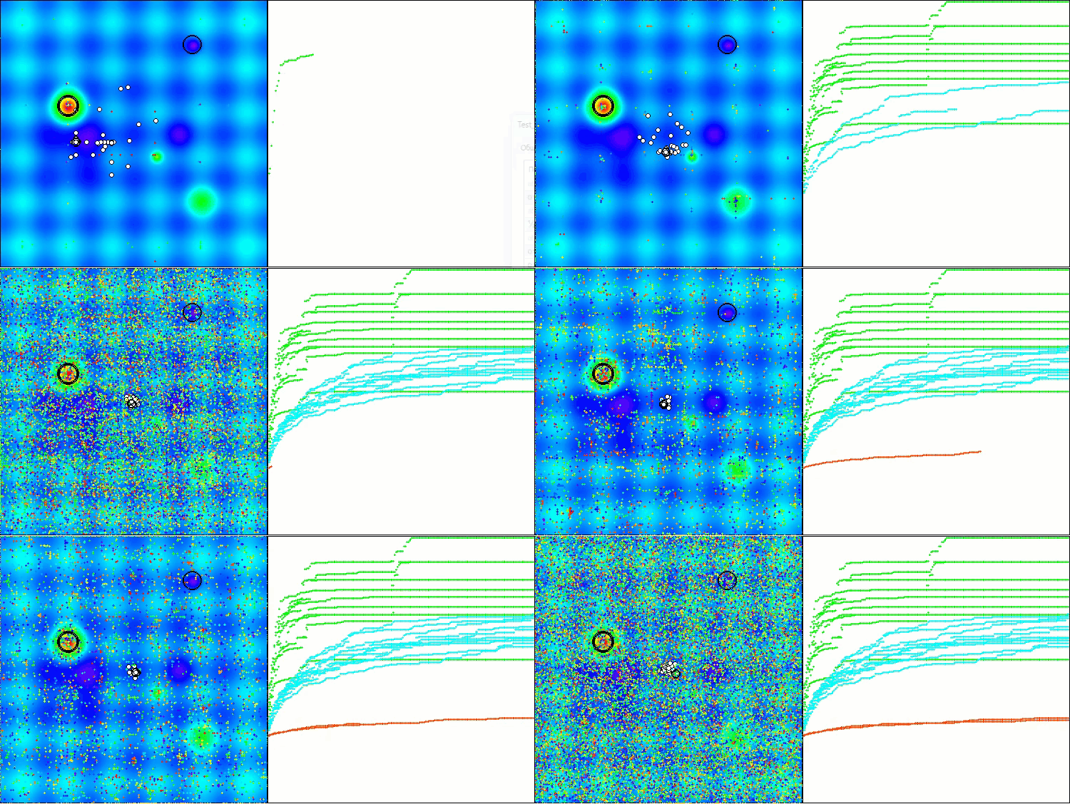
BIO on the Hilly test function

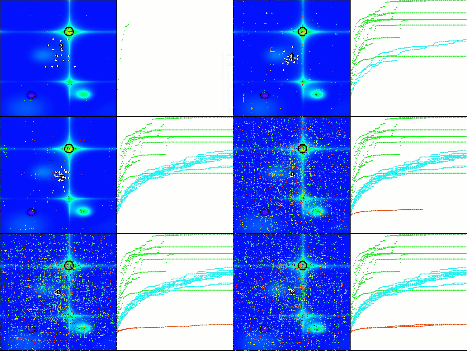
BIO on the Forest test function

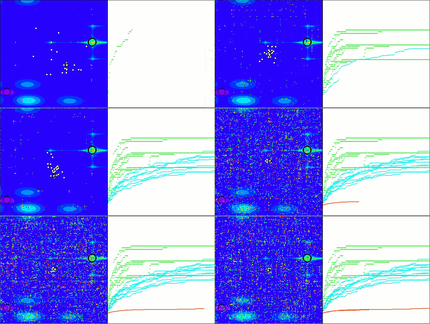
BIO on the Megacity test function

Based on the test results, the BIO algorithm occupies 20th position in the ranking table of population optimization algorithms.

#	AO	Description	Hilly			Hilly final	Forest			Forest final	Megacity (discrete)			Megacity final	Final result	% of MAX
			10 p (5 F)	50 p (25 F)	1000 p (500 F)		10 p (5 F)	50 p (25 F)	1000 p (500 F)		10 p (5 F)	50 p (25 F)	1000 p (500 F)
1	ANS	across neighbourhood search	0.94948	0.84776	0.43857	2.23581	1.00000	0.92334	0.39988	2.32323	0.70923	0.63477	0.23091	1.57491	6.134	68.15
2	CLA	code lock algorithm (joo)	0.95345	0.87107	0.37590	2.20042	0.98942	0.91709	0.31642	2.22294	0.79692	0.69385	0.19303	1.68380	6.107	67.86
3	AMOm	animal migration ptimization M	0.90358	0.84317	0.46284	2.20959	0.99001	0.92436	0.46598	2.38034	0.56769	0.59132	0.23773	1.39675	5.987	66.52
4	(P+O)ES	(P+O) evolution strategies	0.92256	0.88101	0.40021	2.20379	0.97750	0.87490	0.31945	2.17185	0.67385	0.62985	0.18634	1.49003	5.866	65.17
5	CTA	comet tail algorithm (joo)	0.95346	0.86319	0.27770	2.09435	0.99794	0.85740	0.33949	2.19484	0.88769	0.56431	0.10512	1.55712	5.846	64.96
6	TETA	time evolution travel algorithm (joo)	0.91362	0.82349	0.31990	2.05701	0.97096	0.89532	0.29324	2.15952	0.73462	0.68569	0.16021	1.58052	5.797	64.41
7	SDSm	stochastic diffusion search M	0.93066	0.85445	0.39476	2.17988	0.99983	0.89244	0.19619	2.08846	0.72333	0.61100	0.10670	1.44103	5.709	63.44
8	AAm	archery algorithm M	0.91744	0.70876	0.42160	2.04780	0.92527	0.75802	0.35328	2.03657	0.67385	0.55200	0.23738	1.46323	5.548	61.64
9	ESG	evolution of social groups (joo)	0.99906	0.79654	0.35056	2.14616	1.00000	0.82863	0.13102	1.95965	0.82333	0.55300	0.04725	1.42358	5.529	61.44
10	SIA	simulated isotropic annealing (joo)	0.95784	0.84264	0.41465	2.21513	0.98239	0.79586	0.20507	1.98332	0.68667	0.49300	0.09053	1.27020	5.469	60.76
11	ACS	artificial cooperative search	0.75547	0.74744	0.30407	1.80698	1.00000	0.88861	0.22413	2.11274	0.69077	0.48185	0.13322	1.30583	5.226	58.06
12	DA	dialectical algorithm	0.86183	0.70033	0.33724	1.89940	0.98163	0.72772	0.28718	1.99653	0.70308	0.45292	0.16367	1.31967	5.216	57.95
13	BHAm	black hole algorithm M	0.75236	0.76675	0.34583	1.86493	0.93593	0.80152	0.27177	2.00923	0.65077	0.51646	0.15472	1.32195	5.196	57.73
14	ASO	anarchy society optimization	0.84872	0.74646	0.31465	1.90983	0.96148	0.79150	0.23803	1.99101	0.57077	0.54062	0.16614	1.27752	5.178	57.54
15	RFO	royal flush optimization (joo)	0.83361	0.73742	0.34629	1.91733	0.89424	0.73824	0.24098	1.87346	0.63154	0.50292	0.16421	1.29867	5.089	56.55
16	AOSm	atomic orbital search M	0.80232	0.70449	0.31021	1.81702	0.85660	0.69451	0.21996	1.77107	0.74615	0.52862	0.14358	1.41835	5.006	55.63
17	TSEA	turtle shell evolution algorithm (joo)	0.96798	0.64480	0.29672	1.90949	0.99449	0.61981	0.22708	1.84139	0.69077	0.42646	0.13598	1.25322	5.004	55.60
18	DE	differential evolution	0.95044	0.61674	0.30308	1.87026	0.95317	0.78896	0.16652	1.90865	0.78667	0.36033	0.02953	1.17653	4.955	55.06
19	CRO	chemical reaction optimization	0.94629	0.66112	0.29853	1.90593	0.87906	0.58422	0.21146	1.67473	0.75846	0.42646	0.12686	1.31178	4.892	54.36
20	BIO	blood inheritance optimization (joo)	0.81568	0.65336	0.30877	1.77781	0.89937	0.65319	0.21760	1.77016	0.67846	0.47631	0.13902	1.29378	4.842	53.80
21	BSA	bird swarm algorithm	0.89306	0.64900	0.26250	1.80455	0.92420	0.71121	0.24939	1.88479	0.69385	0.32615	0.10012	1.12012	4.809	53.44
22	HS	harmony search	0.86509	0.68782	0.32527	1.87818	0.99999	0.68002	0.09590	1.77592	0.62000	0.42267	0.05458	1.09725	4.751	52.79
23	SSG	saplings sowing and growing	0.77839	0.64925	0.39543	1.82308	0.85973	0.62467	0.17429	1.65869	0.64667	0.44133	0.10598	1.19398	4.676	51.95
24	BCOm	bacterial chemotaxis optimization M	0.75953	0.62268	0.31483	1.69704	0.89378	0.61339	0.22542	1.73259	0.65385	0.42092	0.14435	1.21912	4.649	51.65
25	ABO	african buffalo optimization	0.83337	0.62247	0.29964	1.75548	0.92170	0.58618	0.19723	1.70511	0.61000	0.43154	0.13225	1.17378	4.634	51.49
26	(PO)ES	(PO) evolution strategies	0.79025	0.62647	0.42935	1.84606	0.87616	0.60943	0.19591	1.68151	0.59000	0.37933	0.11322	1.08255	4.610	51.22
27	TSm	tabu search M	0.87795	0.61431	0.29104	1.78330	0.92885	0.51844	0.19054	1.63783	0.61077	0.38215	0.12157	1.11449	4.536	50.40
28	BSO	brain storm optimization	0.93736	0.57616	0.29688	1.81041	0.93131	0.55866	0.23537	1.72534	0.55231	0.29077	0.11914	0.96222	4.498	49.98
29	WOAm	wale optimization algorithm M	0.84521	0.56298	0.26263	1.67081	0.93100	0.52278	0.16365	1.61743	0.66308	0.41138	0.11357	1.18803	4.476	49.74
30	AEFA	artificial electric field algorithm	0.87700	0.61753	0.25235	1.74688	0.92729	0.72698	0.18064	1.83490	0.66615	0.11631	0.09508	0.87754	4.459	49.55
31	AEO	artificial ecosystem-based optimization algorithm	0.91380	0.46713	0.26470	1.64563	0.90223	0.43705	0.21400	1.55327	0.66154	0.30800	0.28563	1.25517	4.454	49.49
32	ACOm	ant colony optimization M	0.88190	0.66127	0.30377	1.84693	0.85873	0.58680	0.15051	1.59604	0.59667	0.37333	0.02472	0.99472	4.438	49.31
33	BFO-GA	bacterial foraging optimization - ga	0.89150	0.55111	0.31529	1.75790	0.96982	0.39612	0.06305	1.42899	0.72667	0.27500	0.03525	1.03692	4.224	46.93
34	SOA	simple optimization algorithm	0.91520	0.46976	0.27089	1.65585	0.89675	0.37401	0.16984	1.44060	0.69538	0.28031	0.10852	1.08422	4.181	46.45
35	ABHA	artificial bee hive algorithm	0.84131	0.54227	0.26304	1.64663	0.87858	0.47779	0.17181	1.52818	0.50923	0.33877	0.10397	0.95197	4.127	45.85
36	ACMO	atmospheric cloud model optimization	0.90321	0.48546	0.30403	1.69270	0.80268	0.37857	0.19178	1.37303	0.62308	0.24400	0.10795	0.97503	4.041	44.90
37	ADAMm	adaptive moment estimation M	0.88635	0.44766	0.26613	1.60014	0.84497	0.38493	0.16889	1.39880	0.66154	0.27046	0.10594	1.03794	4.037	44.85
38	ATAm	artificial tribe algorithm M	0.71771	0.55304	0.25235	1.52310	0.82491	0.55904	0.20473	1.58867	0.44000	0.18615	0.09411	0.72026	3.832	42.58
39	ASHA	artificial showering algorithm	0.89686	0.40433	0.25617	1.55737	0.80360	0.35526	0.19160	1.35046	0.47692	0.18123	0.09774	0.75589	3.664	40.71
40	ASBO	adaptive social behavior optimization	0.76331	0.49253	0.32619	1.58202	0.79546	0.40035	0.26097	1.45677	0.26462	0.17169	0.18200	0.61831	3.657	40.63
41	MEC	mind evolutionary computation	0.69533	0.53376	0.32661	1.55569	0.72464	0.33036	0.07198	1.12698	0.52500	0.22000	0.04198	0.78698	3.470	38.55
42	CSA	circle search algorithm	0.66560	0.45317	0.29126	1.41003	0.68797	0.41397	0.20525	1.30719	0.37538	0.23631	0.10646	0.71815	3.435	38.17
43	IWO	invasive weed optimization	0.72679	0.52256	0.33123	1.58058	0.70756	0.33955	0.07484	1.12196	0.42333	0.23067	0.04617	0.70017	3.403	37.81
44	Micro-AIS	micro artificial immune system	0.79547	0.51922	0.30861	1.62330	0.72956	0.36879	0.09398	1.19233	0.37667	0.15867	0.02802	0.56335	3.379	37.54
45	COAm	cuckoo optimization algorithm M	0.75820	0.48652	0.31369	1.55841	0.74054	0.28051	0.05599	1.07704	0.50500	0.17467	0.03380	0.71347	3.349	37.21
	RW	random walk	0.48754	0.32159	0.25781	1.06694	0.37554	0.21944	0.15877	0.75375	0.27969	0.14917	0.09847	0.52734	2.348	26.09

Summary

While developing and testing the Blood Inheritance Optimization (BIO) algorithm, I came to several important conclusions. First of all, the use of blood group inheritance association has proven to be a successful approach to organizing different mutation strategies in the population optimization algorithm. Testing on various functions and dimensions showed that the algorithm is quite versatile and capable of working effectively with both simple, low-dimensional problems and more complex, multidimensional ones.

It is especially important to note that the presented BIO implementation is only a basic version demonstrating the concept. The key idea of the algorithm lies not so much in the specific mutation operators (which can be replaced with any others), but in the very structure of inheritance of strategies for changing parameters through an analogy with blood groups. This opens up wide possibilities for modification and expansion of the algorithm. Each "blood group" can be associated with any other mutation operators, borrowed from other algorithms or created for a specific task. Moreover, we can experiment with the number of "blood groups", adding new strategies or combining existing ones.

Current test results, showing a respectable position in the ranking of population algorithms (with a score of about 54%), indicate the efficiency of the approach even in its basic implementation. The observed tendency to get stuck in local optima can be overcome by modifying the mutation operators or adding new strategies for exploring the solution space.

I see the most promising direction for the algorithm's development in the creation of adaptive versions, where the mutation operators for each "blood type" can dynamically change during the optimization process, adapting to the landscape of the target function. It is also interesting to explore the possibility of using different inheritance patterns other than the classical ABO blood group system, which could lead to the creation of a whole family of algorithms based on different biological inheritance systems.

Thus, BIO is not just another optimization algorithm, but a flexible conceptual basis for creating a family of algorithms united by the common idea of inheriting solution search strategies through the metaphor of blood groups and opens up wide opportunities for further research and modifications aimed at improving the algorithm's efficiency in various application areas.

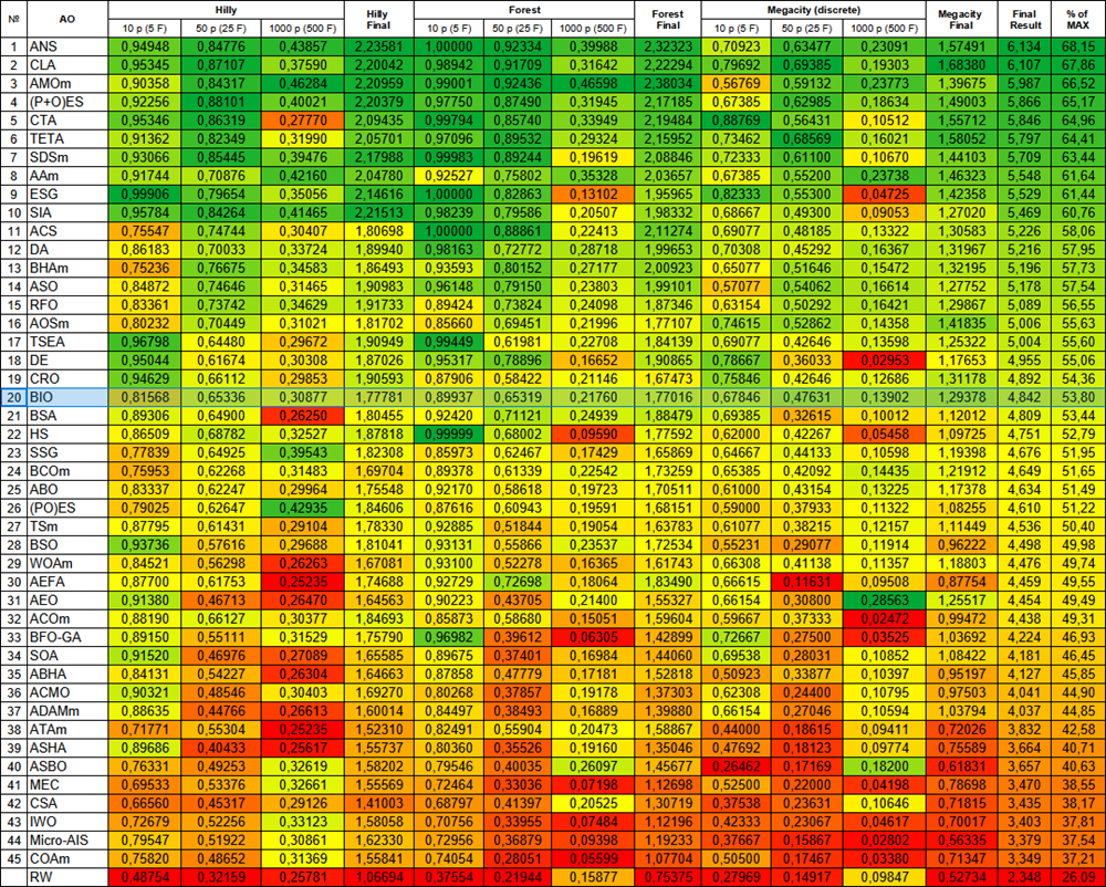
Figure 2. Color gradation of algorithms according to the corresponding tests

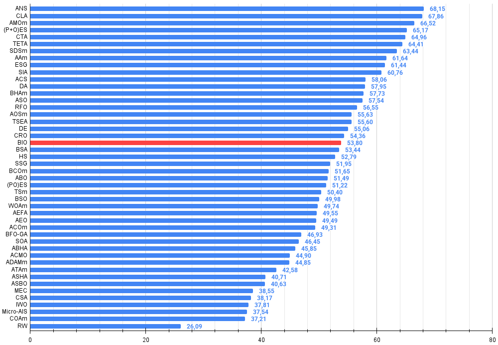
Figure 3. Histogram of algorithm testing results (scale from 0 to 100, the higher the better, where 100 is the maximum possible theoretical result, in the archive there is a script for calculating the rating table)

BIO pros and cons:

Pros:

1. No external parameters
2. Interesting idea about inheritance by blood groups
   
3. Good convergence on high and medium dimensional functions

Disadvantages:

1. Gets stuck at local extremes on low-dimensional problems.
   

The article is accompanied by an archive with the current versions of the algorithm codes. The author of the article is not responsible for the absolute accuracy in the description of canonical algorithms. Changes have been made to many of them to improve search capabilities. The conclusions and judgments presented in the articles are based on the results of the experiments.

• github: https://github.com/JQSakaJoo/Population-optimization-algorithms-MQL5

Programs used in the article

#	Name	Type	Description
1	#C_AO.mqh	Include	Parent class of population optimization algorithms
2	#C_AO_enum.mqh	Include	Enumeration of population optimization algorithms
3	TestFunctions.mqh	Include	Library of test functions
4	TestStandFunctions.mqh	Include	Test stand function library
5	Utilities.mqh	Include	Library of auxiliary functions
6	CalculationTestResults.mqh	Include	Script for calculating results in the comparison table
7	Testing AOs.mq5	Script	The unified test stand for all population optimization algorithms
8	Simple use of population optimization algorithms.mq5	Script	A simple example of using population optimization algorithms without visualization
9	Test_AO_BIO.mq5	Script	BIO test stand