Population optimization algorithms: Differential Evolution (DE)

Contents

1. Introduction
2. Algorithm
3. Test results

1. Introduction

Metaheuristic optimization methods are a class of algorithms that use heuristic approaches to solve complex optimization problems. They differ from numerical optimization methods, which are usually based on mathematical analysis and require knowledge of the gradient or derivative of the objective function. The main difference between metaheuristic methods is their ability to explore large search spaces and find global optima even when the function has many local optima or is not continuously differentiable. The advantage of metaheuristic methods is that they can work with a "black box" - a function, for which there is no analytical solution. They are based on stochastic probabilistic principles and provide good solution quality.

Evolutionary algorithms (EA) are a separate class of metaheuristic optimization methods that simulate the process of natural evolution to solve complex optimization problems. They are based on the principles of heredity, mutation, crossover and natural selection. The process of evolution in evolutionary algorithms models natural selection, where the fittest solutions are more likely to survive and pass on their characteristics to the next generation. Thus, the population gradually converges to the optimal solution. Some of the most well-known evolutionary algorithms include: genetic algorithms (GA), evolutionary programming (EP), evolutionary strategies (ES) and genetic programming (GP). Each of these algorithms has its own characteristics and is used in various fields.

In general, evolutionary algorithms are a powerful tool for solving complex optimization problems, especially in cases where there is no access to an analytical function expression or gradient. They allow exploring the search space and find optimal solutions by combining information from different individual solutions.

Differential evolution (DE) is one of the metaheuristic optimization methods. It differs from other methods in its simplicity and efficiency. DE uses a population of vectors that mutate and crossbreed to create new solutions. It does not require knowledge of the gradient and is capable of finding global optima.

The DE algorithm was developed in the 90s by Storn and Price (published in "Differential Evolution - A Simple and Efficient Heuristic for global Optimization over Continuous Spaces"), and has since become one of the most popular optimization methods that uses a population of parameter vectors to find the optimal solution.

2. Algorithm

The idea of differential evolution is a combination of simplicity and efficiency. The differential evolution algorithm uses a population of vectors representing potential solutions. Each vector consists of components that represent the values of the optimization problem variables.

In DE, a vector takes the role of the search agent. The algorithm starts by creating a random population of vectors. An iterative process then occurs, in which each vector mutates and crosses with other vectors in the population. Mutation is accomplished by adding the difference between two randomly selected vectors from the population to a third vector. This creates a new vector that represents a potential solution to the problem.

After mutation, the mutated vector is crossed with the original vector. Crossing allows combining information from two vectors and creating new solutions. The obtained result is compared with the current best solution in the population. If the new vector is better, it replaces the old one and becomes part of the population. Mutation allows exploring the search space, while crossing allows combining information from different vectors and creating new solutions.

Mutation, crossbreeding and replacement are repeated over several iterations until a stop condition is reached, such as a given number of iterations or reaching the required solution accuracy (in our case, reaching 10,000 fitness function runs).

DE is one of the evolutionary algorithms widely used to solve optimization problems. The differential algorithm uses the differentiation operator to create new candidates based on the current population. Here are the basic equations used in the differential algorithm:

1. Equation for creating a new candidate (differentiation):

r = r1 + F * (r2 - r3)

where:

• v - new vector component
• r1, r2 and r3 - components of randomly selected vectors (individual solutions from the population)
• F - differentiation ratio, which controls the degree of the solution variability (scatter of obtained values). The default range is (0.0;1.0]
  

2. Crossover equation:

u = crossover (x, v)

Equation describes the crossover between the current solution x and the new candidate v. The crossover operator determines which components of the solution will be taken from the new candidate. This is the probability of using a new vector component, otherwise the component remains unchanged. The values (0.0;1.0] are used.

Let's write a pseudocode for the DE algorithm, which is simple and understandable due to the simplicity of the algorithm itself (in fact, the code will be just a bit more complex than its pseudocode):

1. Create a random population of vectors
   
2. Calculate the fitness function
3. Update the best solution
4. Update the population (replace vectors with better mutants)
5. Create a mutant vector component or leave the same one depending on which one is better
   
6. Repeat from p. 2.

To describe a vector in the DE algorithm, we will write a structure and call it S_Vector, which is a vector in n-dimensional space. The structure has the following fields:

•  Init (int coords): the function initializes the 'coords' specified length vector. It creates two arrays - "c" and "cPrev", representing the vector's coordinates and its previous coordinates, respectively. Also the initial values for f and fPrev are set to -DBL_MAX. 
• c []: array containing vector coordinates
• cPrev []: array containing vector coordinates at the previous iteration 
• f: fitness function value for the current vector 
• fPrev: value of the vector fitness function at the previous iteration

//——————————————————————————————————————————————————————————————————————————————
struct S_Vector
{
  void Init (int coords)
  {
    ArrayResize (c,     coords);
    ArrayResize (cPrev, coords);
    f        = -DBL_MAX;
    fPrev    = -DBL_MAX;
  }

  double c     []; //coordinates
  double cPrev []; //previous coordinates
  double f;        //fitness
  double fPrev;    //previous fitness
};
//——————————————————————————————————————————————————————————————————————————————

The class description for such an elementary algorithm as DE is also very simple. Let’s declare the class C_AO_DE. The fields of the C_AO_DE class contain information about the current state of the algorithm and its parameters, and the methods perform various operations related to optimizing the function.

The class has the following fields and methods:

• cB []: array contains the best coordinates found by the algorithm
• fB: fitness function value for the best coordinates
• v []: array of S_Vector structures representing a population of vectors
• rangeMax[]: array stores the maximum values for each vector coordinate
• rangeMin[]: the array contains minimum values for each vector coordinate
• rangeStep[]: array contains step values for each vector coordinate
• Init (int coordsP, int popSizeP, double diffWeightP, double crossProbabP): function initializes the algorithm parameters. It takes the "coordsP" number of coordinates, the "popSizeP" population size, the "diffWeightP" differential weight and the "crossProbabP" crossover probability.
• Moving (): the function performs one step of the differential evolution algorithm
• Revision (): the function performs a revision of the vector population
• SeInDiSp (double In, double InMin, double InMax, double Step): the method calculates a new coordinate value in a given range with a given step
• RNDfromCI (double min, double max): the function generates a random number in the range [min, max]

//——————————————————————————————————————————————————————————————————————————————
class C_AO_DE
{
  //----------------------------------------------------------------------------
  public: double cB  []; //best coordinates
  public: double fB;     //FF of the best coordinates
  public: S_Vector v []; //vector

  public: double rangeMax  []; //maximum search range
  public: double rangeMin  []; //manimum search range
  public: double rangeStep []; //step search

  public: void Init (const int    coordsP,       //coordinates number
                     const int    popSizeP,      //population size
                     const double diffWeightP,   //differential weight
                     const double crossProbabP); //crossover robability

  public: void Moving   ();
  public: void Revision ();

  //----------------------------------------------------------------------------
  private: int    coords;       //coordinates number
  private: int    popSize;      //population size

  private: double diffWeight;   //differential weight
  private: double crossProbab;  //crossover robability

  private: bool   revision;

  private: double SeInDiSp  (double In, double InMin, double InMax, double Step);
  private: double RNDfromCI (double min, double max);
};
//——————————————————————————————————————————————————————————————————————————————

The Init method of the C_AO_DE class initializes the parameters of the differential evolution algorithm. The method takes four parameters:

• coordsP - number of coordinates,
• popSizeP - population size,
• diffWeightP - differential weight
• crossProbabP - crossover probability.

At the beginning, the method uses the MathSrand function to reset the random number generator. This ensures that each time the algorithm is launched, it uses a new sequence of random numbers.

Next, the method initializes the "fB" and "revision" variables. The "fB" variable contains the best fitness function value found by the algorithm. Initially, it is set to "-DBL_MAX", that is, to a very small number. The "revision" variable is set to 'false', which means that the vector population has not been revised yet.

The method then initializes the "coords", "popSize", "diffWeight" and "crossProbab" variables with the values passed as parameters.

The method then creates an array "v" of "popSize" size that contains a population of vectors.

Next, the method creates three arrays: "rangeMax", "rangeMin" and "rangeStep" of 'coords' size (number of coordinates) each.

Finally, the method creates the "cB" array of 'coords' size, which contains the best coordinates found by the algorithm.

//——————————————————————————————————————————————————————————————————————————————
void C_AO_DE::Init  (const int    coordsP,      //coordinates number
                     const int    popSizeP,     //population size
                     const double diffWeightP,  //differential weight
                     const double crossProbabP) //crossover robability
{
  MathSrand ((int)GetMicrosecondCount ()); // reset of the generator
  fB       = -DBL_MAX;
  revision = false;

  coords  = coordsP;
  popSize = popSizeP;

  diffWeight  = diffWeightP;
  crossProbab = crossProbabP;

  ArrayResize (v, popSize);
  for (int i = 0; i < popSize; i++) v [i].Init (coords);

  ArrayResize (rangeMax,  coords);
  ArrayResize (rangeMin,  coords);
  ArrayResize (rangeStep, coords);
  ArrayResize (cB,        coords);
}
//——————————————————————————————————————————————————————————————————————————————

To change the solution vectors in the search space, we will write the Moving method of the C_AO_DE class. The method applies mutation and crossover operators to generate new candidate vectors and selects the best solution based on the fitness function.

The first block of code that begins with the "if (!revision)" condition is executed only the first time the "Moving" method is run or after the Init method is called. It initializes the initial population of vectors with random values within the given limits and with the step specified in the "rangeStep" array.

The method then uses the "for" loop to update each vector in the population. For each vector, the method selects three different random vectors from the population (r1, r2, r3) that are not the same as the current vector (i) and applies mutation and crossover operators to obtain a new candidate vector. The mutation operator calculates the difference between vectors "r2" and "r3" multiplied by the differential weight "diffWeight" and adds the result to the "r1" vector. The crossover operator selects a vector coordinate and replaces it with the corresponding coordinate of a new candidate vector with the crossProbab probability. If the crossover probability does not hold, then the current vector coordinate remains unchanged.

If you parse the code below, you will find that the Moving method of changing vectors does not provide for the creation of coordinates in space, other than those that can be obtained from existing ones. Thus, the stochasticity of the algorithm lies only in the choice of vectors for crossing, but not in the creation of new, original ones. This feature determines far-reaching consequences we will discuss below.

//——————————————————————————————————————————————————————————————————————————————
void C_AO_DE::Moving ()
{
  //----------------------------------------------------------------------------
  if (!revision)
  {
    for (int i = 0; i < popSize; i++)
    {
      for (int c = 0; c < coords; c++)
      {
        v [i].c [c] = RNDfromCI (rangeMin [c], rangeMax [c]);
        v [i].c [c] = SeInDiSp (v [i].c [c], rangeMin [c], rangeMax [c], rangeStep [c]);
      }
    }

    revision = true;
    return;
  }

  //----------------------------------------------------------------------------
  double rnd = 0.0;
  int    r   = 0;
  int    r1  = 0;
  int    r2  = 0;
  int    r3  = 0;

  for (int i = 0; i < popSize; i++)
  {
    do
    {
      r = (int)RNDfromCI (0, popSize);
      if (r >= popSize) r = popSize - 1;

      r1 = r;
    }
    while (r1 == i);

    do
    {
      r = (int)RNDfromCI (0, popSize);
      if (r >= popSize) r = popSize - 1;

      r2 = r;
    }
    while (r2 == i || r2 == r1);

    do
    {
      r = (int)RNDfromCI (0, popSize);
      if (r >= popSize) r = popSize - 1;

      r3 = r;
    }
    while (r3 == i || r3 == r1 || r3 == r2);

    for (int c = 0; c < coords; c++)
    {
      rnd = RNDfromCI (0, 1.0);

      if (rnd < crossProbab)
      {
        v [i].c [c] = v [r1].cPrev [c] + diffWeight * (v [r2].cPrev [c] - v [r3].cPrev [c]);
        v [i].c [c] = SeInDiSp (v [i].c [c], rangeMin [c], rangeMax [c], rangeStep [c]);
      }
      else
      {
        v [i].c [c] = v [i].cPrev [c];
      }
    }
  }
}
//——————————————————————————————————————————————————————————————————————————————

Finally, we need the Revision method of the C_AO_DE class, which updates the best solution in the population and saves the previous values of the fitness function and vector coordinates.

First, the method initializes the "ind" variable with the value "-1". It then uses the "for" loop to iterate over all the vectors in the population. If the fitness function of the current vector is greater than "fB" (the best fitness function found so far), it stores the index of that vector in the "ind" variable.

If "ind" is not equal to "-1", then the method updates the value of "fB" to the value of the fitness function of the vector with the "ind" index and stores its coordinates in the "cB" array.

The method then uses another "for" loop to iterate through all the vectors in the population. If the fitness function of the current vector is greater than its previous value, then the method stores the current value of the fitness function and the vector coordinates in the corresponding v[i].fPrev and v[i].cPrev fields.

This method allows the C_AO_DE class to store the best solution in the population and the previous values of the fitness function and vector coordinates for later use in optimizing the fitness function.

We can see that the population will not move any further in the search space until a vector better than its original (parent) version is found. This point complements all that was said above.

//——————————————————————————————————————————————————————————————————————————————
void C_AO_DE::Revision ()
{
  //----------------------------------------------------------------------------
  int ind = -1;

  for (int i = 0; i < popSize; i++)
  {
    if (v [i].f > fB) ind = i;
  }

  if (ind != -1)
  {
    fB = v [ind].f;
    ArrayCopy (cB, v [ind].c, 0, 0, WHOLE_ARRAY);
  }

  //----------------------------------------------------------------------------
  for (int i = 0; i < popSize; i++)
  {
    if (v [i].f > v [i].fPrev)
    {
      v [i].fPrev = v [i].f;
      ArrayCopy (v [i].cPrev, v [i].c, 0, 0, WHOLE_ARRAY);
    }
  }
}
//——————————————————————————————————————————————————————————————————————————————

3. Test results

DE test stand results:

C_AO_DE:50;0.2;0.8
=============================
5 Rastrigin's; Func runs 10000 result: 80.30183306326985
Score: 0.99498
25 Rastrigin's; Func runs 10000 result: 76.15178282331799
Score: 0.94356
500 Rastrigin's; Func runs 10000 result: 52.17316317703311
Score: 0.64645
=============================
5 Forest's; Func runs 10000 result: 1.7348423083855402
Score: 0.98131
25 Forest's; Func runs 10000 result: 1.28572746338484
Score: 0.72727
500 Forest's; Func runs 10000 result: 0.20833645141168078
Score: 0.11785
=============================
5 Megacity's; Func runs 10000 result: 9.640000000000002
Score: 0.80333
25 Megacity's; Func runs 10000 result: 3.9199999999999995
Score: 0.32667
500 Megacity's; Func runs 10000 result: 0.3548
Score: 0.02957
=============================
All score: 5.57100

We see excellent test results based on the output values of the algorithm.

We can see the phenomenal convergence of the algorithm, but we can also notice the feature that was mentioned above in the description of the Moving and Revision methods. When creating the visualization, after several attempts, I specifically chose the most successful ones. In fact, the results are not always so outstanding. This is explained by the degeneration of the population, when the entire population, every single vector, converges to a single extremum. But this may not be the global optimum at all. As mentioned above, the algorithm does not have mechanisms to continue exploring the search space, creating new unique vectors. The DE algorithm does not create new vectors, but only generates combinations from existing ones. This explains the complete degeneration. No "new blood" is created to diversify the "gene pool" of the population.

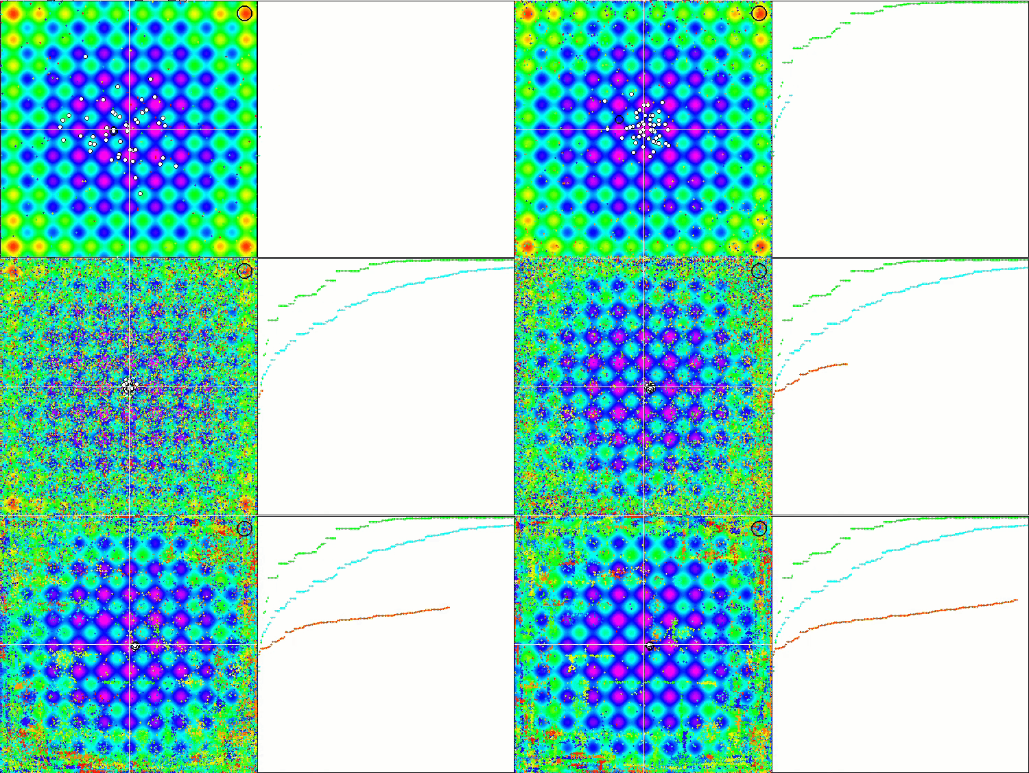
  DE on the Rastrigin test function.

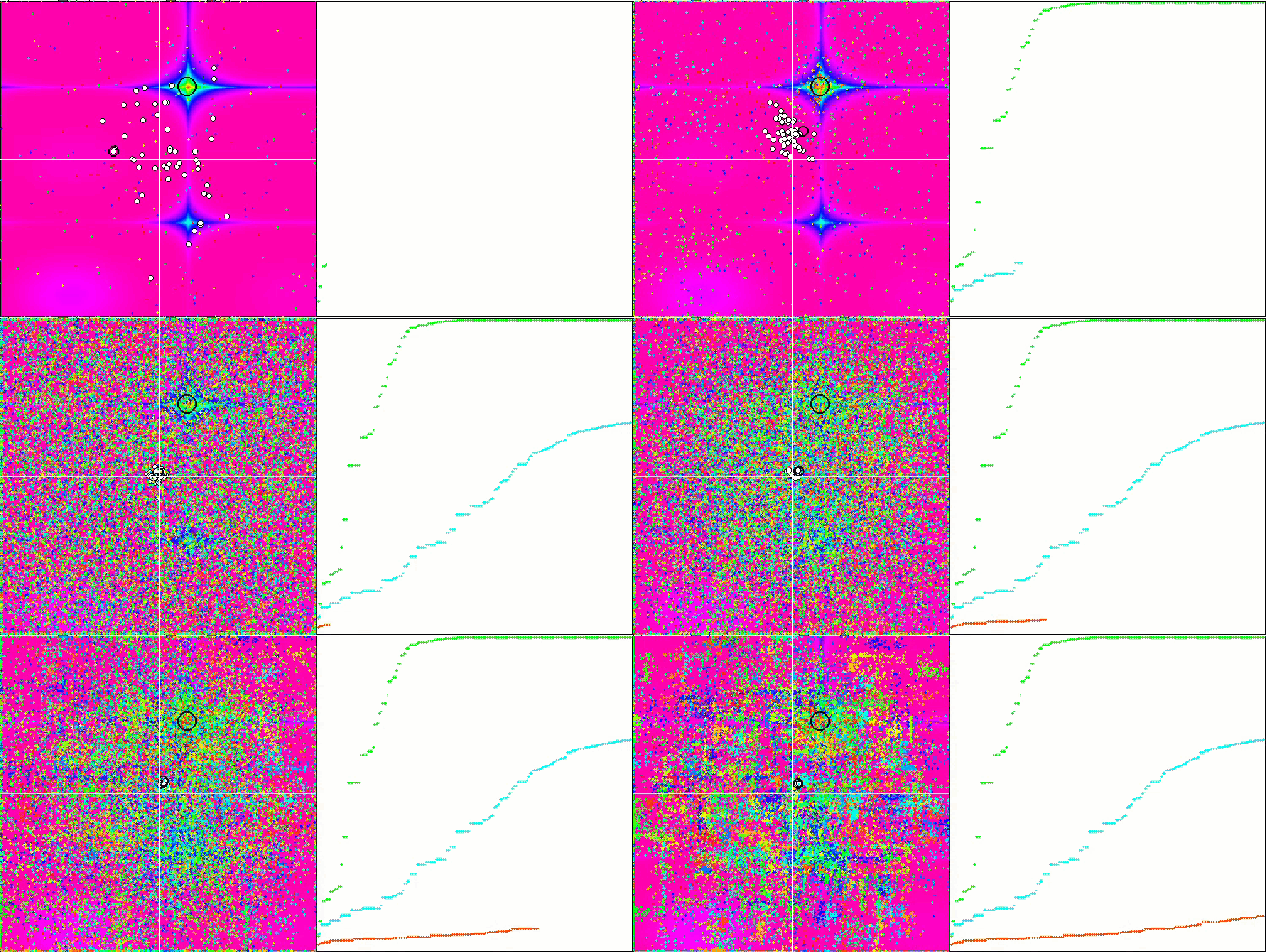
  DE on the Forest test function.

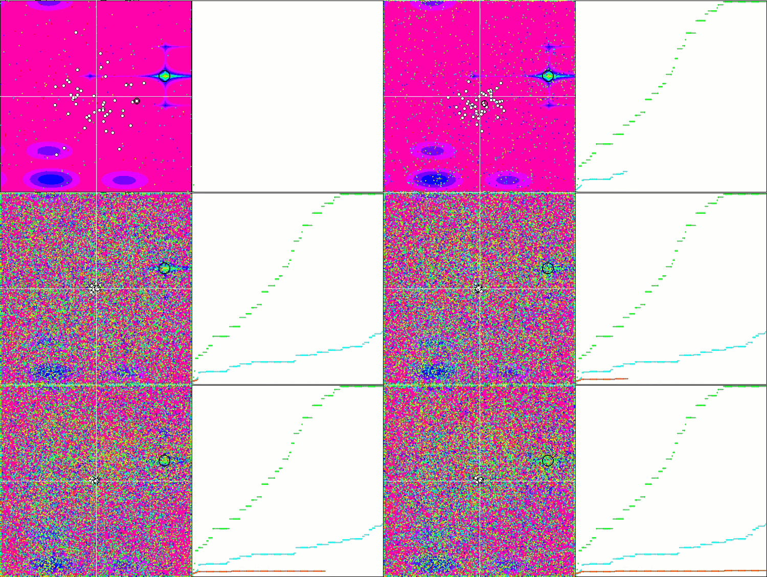
  DE on the Megacity test function.

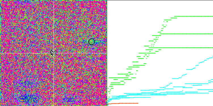
Huge spread of convergence. Especially noticeable in the Forest and Megacity functions

Let's move on to consider the final rating table with the new participant - DE. The algorithm was able to snatch the top spot from the current leader SDSm in the Forest test with 10 variables. The results of other tests are also very good and DE took fourth place after SSG. It should be noted that instead of the usual 5-fold test run for each of the test functions, I had to perform the 10-fold test due to the huge scatter of results on the Forest and Megacity functions. On the smooth Rastrigin function, the scatter of the results is less noticeable. 

#	AO	Description	Rastrigin			Rastrigin final	Forest			Forest final	Megacity (discrete)			Megacity final	Final result
			10 p (5 F)	50 p (25 F)	1000 p (500 F)		10 p (5 F)	50 p (25 F)	1000 p (500 F)		10 p (5 F)	50 p (25 F)	1000 p (500 F)
1	SDSm	stochastic diffusion search M	0.99809	1.00000	0.69149	2.68958	0.99265	1.00000	1.00000	2.99265	1.00000	1.00000	1.00000	3.00000	100.000
2	SDS	stochastic Diffusion Search	0.99737	0.97322	0.58904	2.55963	0,96067	0.93572	0.79649	2.69288	0.78696	0.93815	0.71804	2.44315	88.201
3	SSG	saplings sowing and growing	1.00000	0.92761	0.51630	2.44391	0.72120	0.65201	0.83760	2.21081	0.54782	0.61841	0.99522	2.16146	77.683
4	DE	differential evolution	0.98295	0.89236	0.51375	2.38906	1.00000	0.84602	0.65510	2.50112	0.90000	0.52237	0.12031	1.54268	73.099
5	HS	harmony search	0.99676	0.88385	0.44686	2.32747	0.99148	0.68242	0.37529	2.04919	0.71739	0.71842	0.41338	1.84919	70.623
6	IWO	invasive weed optimization	0.95828	0.62227	0.27647	1.85703	0.70170	0.31972	0.26613	1.28755	0.57391	0.30527	0.33130	1.21048	48.250
7	ACOm	ant colony optimization M	0.34611	0.16683	0.15808	0.67103	0.86147	0.68980	0.64798	2.19925	0.71739	0.63947	0.05579	1.41265	47.387
8	MEC	mind evolutionary computation	0.99270	0.47345	0.21148	1.67763	0.60244	0.28046	0.21324	1.09615	0.66957	0.30000	0.26045	1.23002	44.049
9	SDOm	spiral dynamics optimization M	0.69840	0.52988	0.33168	1.55996	0.59818	0.38766	0.37600	1.36183	0.35653	0.15262	0.25842	0.76758	40.289
10	COAm	cuckoo optimization algorithm M	0.92400	0.43407	0.24120	1.59927	0.57881	0.23477	0.13842	0.95200	0.52174	0.24079	0.17001	0.93254	37.830
11	FAm	firefly algorithm M	0.59825	0.31520	0.15893	1.07239	0.50637	0.29178	0.41704	1.21519	0.24783	0.20526	0.35090	0.80398	33.139
12	ABC	artificial bee colony	0.78170	0.30347	0.19313	1.27829	0.53379	0.14799	0.11177	0.79355	0.40435	0.19474	0.13859	0.73768	29.766
13	BA	bat algorithm	0.40526	0.59145	0.78330	1.78002	0.20664	0.12056	0.21769	0.54488	0.21305	0.07632	0.17288	0.46225	29.499
14	CSS	charged system search	0.56605	0.68683	1.00000	2.25289	0.13961	0.01853	0.13638	0.29452	0.07392	0.00000	0.03465	0.10856	27.930
15	GSA	gravitational search algorithm	0.70167	0.41944	0.00000	1.12111	0.31390	0.25120	0.27812	0.84322	0.42609	0.25525	0.00000	0.68134	27.807
16	BFO	bacterial foraging optimization	0.67203	0.28721	0.10957	1.06881	0.39364	0.18364	0.17298	0.75026	0.37392	0.24211	0.18841	0.80444	27.542
17	EM	electroMagnetism-like algorithm	0.12235	0.42928	0.92752	1.47915	0.00000	0.02413	0.29215	0.31628	0.00000	0.00527	0.10872	0.11399	19.002
18	SFL	shuffled frog-leaping	0.40072	0.22021	0.24624	0.86717	0.19981	0.02861	0.02221	0.25063	0.19565	0.04474	0.06607	0.30646	13.200
19	MA	monkey algorithm	0.33192	0.31029	0.13582	0.77804	0.09927	0.05443	0.07482	0.22852	0.15652	0.03553	0.10669	0.29874	11.777
20	FSS	fish school search	0.46812	0.23502	0.10483	0.80798	0.12730	0.03458	0.05458	0.21647	0.12175	0.03947	0.08244	0.24366	11.332
21	IWDm	intelligent water drops M	0.26459	0.13013	0.07500	0.46972	0.28358	0.05445	0.05112	0.38916	0.22609	0.05659	0.05054	0.33322	10.423
22	PSO	particle swarm optimisation	0.20449	0.07607	0.06641	0.34696	0.18734	0.07233	0.18207	0.44175	0.16956	0.04737	0.01947	0.23641	8.426
23	RND	random	0.16826	0.09038	0.07438	0.33302	0.13381	0.03318	0.03949	0.20648	0.12175	0.03290	0.04898	0.20363	5.054
24	GWO	grey wolf optimizer	0.00000	0.00000	0.02093	0.02093	0.06514	0.00000	0.00000	0.06514	0.23478	0.05789	0.02545	0.31812	1.000

Summary

The differential evolution algorithm is able to find global optima very quickly and has excellent convergence, given the very mediocre results in individual tests. DE is widely used in various fields such as optimization of model parameters, tuning of neural networks, optimization of functions in physics and economics, and many others. I would recommend doing multiple optimization runs with this algorithm, since the results are very dependent on the initial population in the first iteration. Increasing the population size while simultaneously increasing the number of iterations may be beneficial.

Despite its simplicity and operation speed, the differential evolution algorithm has obvious disadvantages, such as degeneration of the population and, as a consequence, getting stuck in local extrema. It is necessary to take that into account when choosing DE for your optimization problems.

The DE algorithm discussed in this article is a kind of template used to create several modifications. My suggestions to improve the differential evolution (DE) algorithm are as follows:

1. Using adaptive parameter control methods: DE has several parameters that need to be adjusted due to their significant impact on the results.

The differential weight parameter recommended by the authors is "0.2". This value is the default value I adopted in the DE testing script. This parameter has a significant impact on the diversity of the population. If we choose a value less than "0.2", we can get even better convergence of the algorithm, but at the same time face even greater scatter in the results. Conversely, if we increase the value of this parameter, then the algorithm becomes resistant to population degeneration and getting stuck in local extrema, but at the same time, the quality of convergence rapidly decreases over the number of iterations limited by tests, and accordingly, the search time inevitably increases.

Crossover probability also affects the optimization quality. The author recommend the value of "0.9". However, my experiments show that "0.8" is more suitable. 

Considering the above, it seems advisable to use adaptive methods to control and dynamically change parameters so that the algorithm can be automatically adjusted depending on the task.

2. Using different mutation and crossover strategies.

3. Use of hybrid methods: DE can be combined with other optimization methods, such as genetic algorithms, gradient-based optimization methods, particle swarm optimization methods, etc. This can improve the performance of the algorithm and help improve the efficiency of the algorithm as a whole.

4. Improving convergence: applying additional random vector generation to increase diversity in a population.

5. Using different strategies for selecting individuals for mutation: this algorithm considers a completely random method for selecting individuals for the crossover. However, this method can also be supplemented or completely replaced by using other different strategies for selecting individuals for crossover/mutation, such as the strategy for selecting individuals based on their suitability. This can help improve population diversity and significantly improve the algorithm resistance to getting stuck.

Overall, the DE algorithm gives a very good impression of its performance, but it is necessary to either keep the features of this interesting algorithm in mind or make some attempts to improve the differential evolution by applying a combination of different strategies and methods. DE has confidently demonstrated that algorithms can be very efficient while still being incredibly simple and fast. The differential evolution algorithm can be recommended for solving complex optimization problems with high dimensions, since the impact of the decrease in diversity during evolution is less pronounced when there are a large number of optimized parameters.

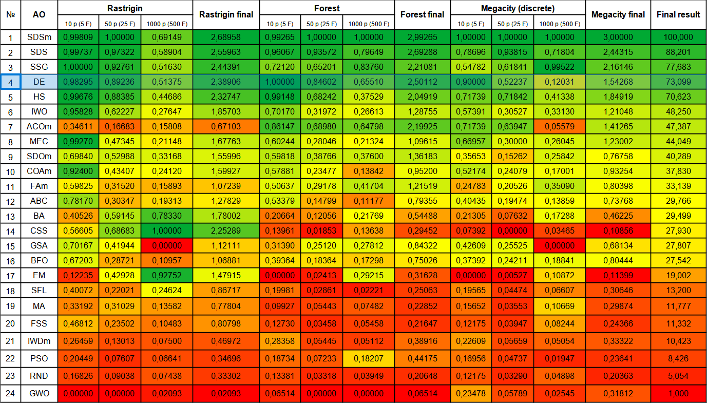
Figure 1. Color gradation of algorithms according to relevant tests

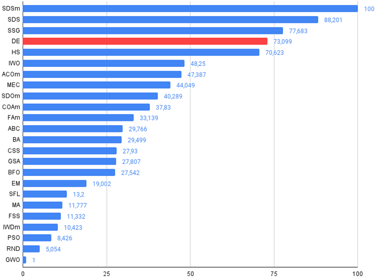
Figure 2. The histogram of algorithm test results (on a scale from 0 to 100, the more the better,

the archive contains the script for calculating the rating table using the method applied in the article).

Pros and cons of the differential evolution (DE) algorithm

Advantages:

1. A small number of external parameters.
2. Simple implementation.
3. Operation speed.
4. Good scalability.
5. Very good performance on various types of functions (taking into account the disadvantages).

Disadvantages:

1. High scatter of results.
2. Tendency to get stuck in local extremes.

The article is accompanied by an archive with updated current versions of the algorithm codes described in previous articles. The author of the article is not responsible for the absolute accuracy in the description of canonical algorithms. Changes have been made to many of them to improve search capabilities. The conclusions and judgments presented in the articles are based on the results of the experiments.