
Artificial Tribe Algorithm (ATA)
Contents
Introduction
As technology rapidly evolves and optimization tasks become more complex, scientists and researchers continue to seek inspiration in nature. One of the striking examples of this approach is the Artificial Tribe Algorithm (ATA), created by scientists T. Chen, Y. Wang and J. Li and published in 2012. Inspired by tribal behavior, ATA uses two main mechanisms - dispersal and migration - to adapt to changing conditions and find optimal solutions to a wide variety of problems. Imagine a vast expanse where groups of people, like their distant ancestors, unite in search of the best resources. They migrate, exchange knowledge and experience, creating unique strategies to solve complex problems. It is this behavior that became the basis for the creation of ATA - the algorithm that harmoniously combines two key mechanisms: distribution and migration.
The Artificial Tribe Algorithm is a completely new optimization method based on the principles of bionic intelligent algorithms. It simulates the behavior of natural tribes, using their reproductive and migratory abilities to achieve optimal solutions. In this algorithm, the tribe consists of individuals who interact with each other to find a global optimum.
Implementation of the algorithm
The ATA algorithm process starts with setting the parameters and randomly initializing the tribe, after which the fitness value is calculated. Next, the iteration counter is incremented and the current situation of the tribe is assessed. If the situation is favorable (the difference in the optimal fitness value between generations is greater than a given criterion), reproduction behavior is performed, where individuals exchange information. Otherwise, migratory behavior is used, in which individuals move based on the experience of both the individual and the entire tribe. Migration cannot be performed continuously to avoid excessive dispersion. The fitness value is then recalculated and compared with the best values recorded for the tribe and each individual. If a better solution is found, it is stored in memory. The termination conditions are checked and if they are met, the iteration is terminated. Otherwise, the process returns to the situation assessment step.
Including global information in ATA adds weight to the tribe's historical experience, helping to find better solutions and improve search capabilities. Increasing the weight of the tribe's experience helps improve the efficiency of the algorithm, accelerating convergence. To achieve this, ATA introduces a global inertial weight, which enhances search capabilities and speeds up the process.
The main innovation of ATA is the presence of a dual behavior system that adapts depending on the situation: reproduction is used for deep exploration when progress is good, and migration is activated when stuck in local optima, which promotes deeper exploration. The combination of individual and social learning is also important. Individual memory (Xs) is used during migration, and global memory (Xg) is weighted by the AT_w inertia factor. During the reproduction, partners are chosen randomly, which helps improve diversity and speed up the search.
The parameter system in ATA is simple but effective. It controls the population size (tribe_size), the behavior switching criterion (AT_criterion) and the global influence on the search (AT_w), making the algorithm flexible and powerful, which, according to the authors, allows it to easily compete with more complex algorithms, especially when dealing with small population sizes.
The main components of the algorithm include a breeding behavior that is applied when progress is good and the difference in fitness is greater than a set criterion. In this case, individuals exchange partial information. Migration behavior is used in a poor situation where the difference in fitness is small, and involves movement based on individual and global experience, taking into account the weight of inertia to enhance global search. The existence criterion evaluates the changes in the best fitness between iterations: if the changes are significant, then reproduction is used, if the changes are insignificant, migration occurs.
The algorithm also includes a memory update system that keeps track of the best positions for both individuals and the entire tribe. These positions are updated when new better solutions are found.
The design features of ATA include simplicity of parameters, integration of individual and social learning, and self-adaptive switching between reproduction and migration. Global inertia weight improves the search performance, speeding up the search for optimal solutions.
So, the rules of individual behavior can be described as follows:
1. Spreading. An individual uses information in a population to form the genetic material of future generations. If the existing environmental situation is favorable, the individual randomly selects another individual from the tribe and interbreeds to produce the next generation through the exchange of genetic information.
2. Migration. If the existing situation is bad (indicating that the intergenerational difference in the optimal fitness value is less than the existing criterion), the individual moves, in accordance with his own and the tribal historical experience, to implement the tribe's migration.
Visually, the key phases occurring in the algorithm population can be schematically represented as follows.
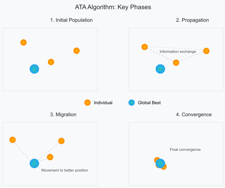
Figure 1. Phases of individual movements in the ATA algorithm population
Let's implement the ATA algorithm pseudocode:
// Main parameters:
// tribe_size - tribe population size
// ATA_criterion - threshold value of the existence criterion
// ATA_w - global inertia weight
// X - vector of the individual's position
// Xs - best historical position of the individual
// Xg - global best historical position of the tribe
ATA algorithm:
Initialization:
Create a tribe of tribe_size individuals with X random positions
Calculate the initial fitness values for all individuals
Initialize Xs and Xg with the best positions found
iteration = 0
While (iteration < max_iterations):
iteration = iteration + 1
// Check if the situation is favorable
difference = |current_best_fitness - previous_best_fitness|
If (difference > ATA_criterion):
// Good situation - perform reproduction behavior
For each i individual:
// Select a random partner j from the tribe
j = random (1, tribe_size) where j ≠ i
// Reproduction equations:
r1 = random (0,1)
Yi+1 = r1 * Yj + (1 - r1) * Xi // New partner position
Xi+1 = r1 * Xi + (1- r1) * Yi // New position of the individual
Otherwise:
// Bad situation - execute migration behavior
For each i individual:
// Migration equation:
r1 = random (0,1)
r2 = random (0,1)
Xi+1 = Xi + r1 * (Xs - Xi) + ATA_w * r2 * (Xg - Xi)
// Update fitness values and best positions
For each i individual:
Calculate new_fitness for Xi
If new_fitness is better than best_fitness_of_individual:
Update Xs for i individual
If new_fitness is better than global_best_fitness:
Update Xg
Save current_best_fitness for next iteration
Return Xg as the best solution found
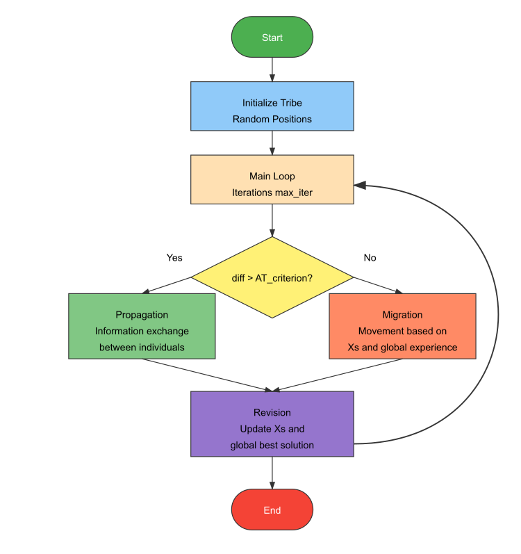
Figure 2. Logical diagram of the ATA algorithm operation
Let's define the C_AO_ATA class that implements the ATA algorithm. Let's briefly describe its contents:
Inheritance and main members:- The class inherits from the C_AO base class
- Contains a destructor and a constructor
- popSize = 50 (tribe size)
- AT_criterion = 0.3 (favorable situation criterion)
- AT_w = 1.46 (inertial weight)
- SetParams () - set parameters from the "params" array
- Init () - initialization with search ranges
- Moving () - implementation of the movement of individuals
- Revision () - evaluate and update solutions
- prevBestFitness - store the previous best value for comparison
This is the basic framework of the algorithm, where all the necessary parameters and methods for its operation are defined.
//——————————————————————————————————————————————————————————————————————————————
class C_AO_ATA : public C_AO
{
  public: //--------------------------------------------------------------------
  ~C_AO_ATA () { }
  C_AO_ATA ()
  {
    ao_name = "ATA";
    ao_desc = "Artificial Tribe Algorithm";
    ao_link = "https://www.mql5.com/en/articles/16588";

    popSize      = 50;   // Population size
    AT_criterion = 0.3;  // Criteria for assessing the current situation
    AT_w         = 1.46; // Global inertial weight

    ArrayResize (params, 3);

    // Initialize parameters
    params [0].name = "popSize";      params [0].val = popSize;
    params [1].name = "AT_criterion"; params [1].val = AT_criterion;
    params [2].name = "AT_w";         params [2].val = AT_w;
  }

  void SetParams () // Method for setting parameters
  {
    popSize      = (int)params [0].val;
    AT_criterion = params     [1].val;
    AT_w         = params     [2].val;
  }

  bool Init (const double &rangeMinP  [], // Minimum search range
             const double &rangeMaxP  [], // Maximum search range
             const double &rangeStepP [], // Search step
             const int     epochsP = 0);  // Number of epochs

  void Moving   ();       // Moving method
  void Revision ();       // Revision method

  //----------------------------------------------------------------------------
  double AT_criterion;    // Criteria for assessing the current situation
  double AT_w;            // Global inertial weight

  private: //-------------------------------------------------------------------
  double prevBestFitness; // Previous best solution
};
//——————————————————————————————————————————————————————————————————————————————
The Init method of the C_AO_ATA class is responsible for initializing the algorithm. Let's break it down into parts:
Method parameters:- rangeMinP [] - array of minimum values for each search dimension
- rangeMaxP [] - array of maximum values
- rangeStepP [] - array of discretization steps
- epochsP - number of epochs (default 0)
- Call StandardInit from the base class to initialize the standard parameters
- If StandardInit returned false, the method is interrupted
- Set prevBestFitness to -DBL_MAX (for the maximization task)
- true in case of successful initialization
- false if the standard initialization fails
This is a minimal implementation of initialization that prepares the algorithm for work.
//——————————————————————————————————————————————————————————————————————————————
bool C_AO_ATA::Init (const double &rangeMinP  [], // Minimum search range
                     const double &rangeMaxP  [], // Maximum search range
                     const double &rangeStepP [], // Search step
                     const int     epochsP = 0)   // Number of epochs
{
  if (!StandardInit (rangeMinP, rangeMaxP, rangeStepP)) return false; // Initialization of standard parameters

  //----------------------------------------------------------------------------
  prevBestFitness = -DBL_MAX;
  return true;
}
//——————————————————————————————————————————————————————————————————————————————
The Moving() method is responsible for the movement of tribe individuals and consists of two main parts:
If this is the first run (revision = false):- Randomly places all individuals in the search space
- brings their positions to acceptable discrete values
- marks that the initial placement is done (revision = true)
- each individual chooses a random partner
- they exchange information about their positions
- form new positions based on this exchange
- your best position
- global best position
- AT_w inertial weight
Whenever there are any movements, all new positions are checked and brought to acceptable values within the specified ranges. Additionally, the following nuance can be noted: since the criterion for assessing the situation is an external parameter and has a dimensionless value, it is necessary to normalize the difference between the current best fitness and the previous one by the difference between the best historical fitness and the worst: diff = (fB - prevBestFitness) / (fB - fW). It is for these purposes that this algorithm tracks not only the globally best solution, but also the globally worst one.
//——————————————————————————————————————————————————————————————————————————————
void C_AO_ATA::Moving ()
{
  // Initial random positioning
  if (!revision) // If there has not been a revision yet
  {
    for (int i = 0; i < popSize; i++) // For each particle
    {
      for (int c = 0; c < coords; c++) // For each coordinate
      {
        a [i].c [c] = u.RNDfromCI (rangeMin [c], rangeMax [c]);                             // Generate random position
        a [i].c [c] = u.SeInDiSp  (a [i].c [c], rangeMin [c], rangeMax [c], rangeStep [c]); // Convert to discrete values
      }
    }

    revision = true; // Set revision flag
    return;          // Exit the method
  }

  //----------------------------------------------------------------------------
  // Check the existence criterion
  double diff = (fB - prevBestFitness) / (fB - fW);

  double Xi   = 0.0;
  double Xi_1 = 0.0;
  double Yi   = 0.0;
  double Yi_1 = 0.0;
  double Xs   = 0.0;
  double Xg   = 0.0;
  int    p    = 0;
  double r1   = 0.0;
  double r2   = 0.0;

  if (diff > AT_criterion)
  {
    // Spread behavior (good situation)
    for (int i = 0; i < popSize; i++)
    {
      for (int c = 0; c < coords; c++)
      {
        p  = u.RNDminusOne (popSize);
        r1 = u.RNDprobab ();

        Xi = a [i].cP [c];
        Yi = a [p].cP [c];

        Xi_1 = r1 * Xi + (1.0 - r1) * Yi;
        Yi_1 = r1 * Yi + (1.0 - r1) * Xi;

        a [i].c [c] = u.SeInDiSp  (Xi_1, rangeMin [c], rangeMax [c], rangeStep [c]);
        a [p].c [c] = u.SeInDiSp  (Yi_1, rangeMin [c], rangeMax [c], rangeStep [c]);
      }
    }
  }
  else
  {
    // Migration behavior (bad situation)
    for (int i = 0; i < popSize; i++)
    {
      for (int c = 0; c < coords; c++)
      {
        r1 = u.RNDprobab ();
        r2 = u.RNDprobab ();

        Xi = a [i].cP [c];
        Xs = a [i].cB [c];
        Xg = cB [c];

        Xi_1 = Xi + r1 * (Xs - Xi) + AT_w * r2 * (Xg - Xi);

        a [i].c [c] = u.SeInDiSp (Xi_1, rangeMin [c], rangeMax [c], rangeStep [c]);
      }
    }
  }
}
//——————————————————————————————————————————————————————————————————————————————
The Revision () is responsible for evaluating and updating the best solutions after moving individuals. Here is what it does:
For all individuals in the tribe:- check whether the global best solution (fB) has been improved
- update the worst solution found (fW)
- check and update each individual's personal best solution (a [i].fB)
- save current positions as previous (in cP)
- save the previous best value (prevBestFitness = tempB)
- copy the coordinates of the best individual into the global best solution (cB)
In essence, this is a method of "auditing" the current state of the tribe, where all important indicators are updated: global best/worst values, personal best values of each individual, and the history of positions is saved.
//——————————————————————————————————————————————————————————————————————————————
void C_AO_ATA::Revision ()
{
  //----------------------------------------------------------------------------
  int    indB  = -1;                // Best particle index
  double tempB = fB;

  for (int i = 0; i < popSize; i++) // For each particle
  {
    if (a [i].f > fB)               // If the function value is better than the current best one
    {
      fB   = a [i].f;               // Update the best value of the function
      indB = i;                     // Save the index of the best particle
    }

    if (a [i].f < fW)               // If the function value is worse than the current worst one
    {
      fW   = a [i].f;               // Update the worst value of the function
    }

    if (a [i].f > a [i].fB)
    {
      a [i].fB = a [i].f;
      ArrayCopy (a [i].cB, a [i].c, 0, 0, WHOLE_ARRAY);
    }

    ArrayCopy (a [i].cP, a [i].c, 0, 0, WHOLE_ARRAY);
  }

  if (indB != -1)
  {
    prevBestFitness = tempB;
    ArrayCopy (cB, a [indB].c, 0, 0, WHOLE_ARRAY); // Copy the coordinates of the best particle
  }
}
//——————————————————————————————————————————————————————————————————————————————
Let's move on to the results of testing the ATA algorithm on the test bench.
ATA|Artificial Tribe Algorithm|50.0|0.3|0.5|
=============================
5 Hilly's; Func runs: 10000; result: 0.540711768815426
25 Hilly's; Func runs: 10000; result: 0.31409437631469717
500 Hilly's; Func runs: 10000; result: 0.2512638813618161
=============================
5 Forest's; Func runs: 10000; result: 0.40309649266442193
25 Forest's; Func runs: 10000; result: 0.2572536671383149
500 Forest's; Func runs: 10000; result: 0.18349902023635473
=============================
5 Megacity's; Func runs: 10000; result: 0.24
25 Megacity's; Func runs: 10000; result: 0.13600000000000004
500 Megacity's; Func runs: 10000; result: 0.09518461538461616
=============================
All score: 2.42110 (26.90%)
As can be seen from the printout of the algorithm's results and the visualization, the algorithm is unable to get into our rating table with the present parameters. The visualization below shows the algorithm's weak ability to escape local traps. The algorithm clearly lacks diversity in the solution population, which leads to its degeneration.
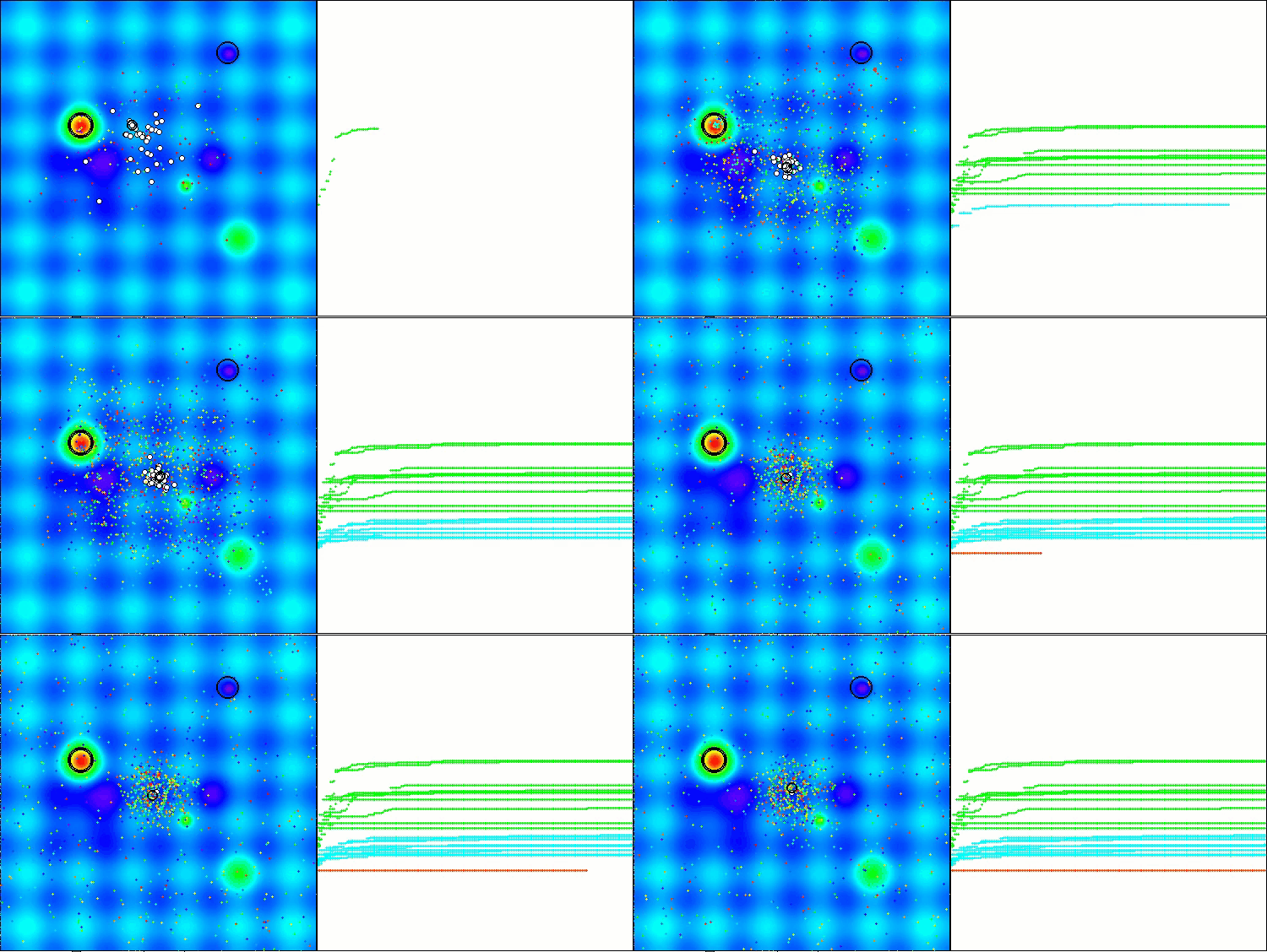
ATAm on the Hilly test functionality
Let's try to improve the ATA algorithm by focusing on the lack of diversity of solutions in the population. This is an important aspect because diversity is key to effectively searching the solution space. In our modification, we will introduce dynamic probability, which will depend on the state of population fitness.
When the population is compressed into a narrow range of the solution space, it can cause the algorithm to get stuck in a local optimum. Just like in the original version of the algorithm, we will track the difference between the current and previous best global solutions, but if this difference turns out to be too small, this will be a signal that the population is not diverse enough and may be approaching solution collapse.
To prevent this situation, we will, with a certain probability, throw out individuals that are far from the current global solution. This will occur within the acceptable boundaries of the task, which will ensure that the conditions of the task are met and prevent it from being exceeded. We will use the normal distribution to determine how far from the current global solution the discarded individuals will be.
Interestingly, the larger the difference between the current and previous best solutions (denoted as "diff"), the higher the probability of such outliers. This will allow us to respond adaptively to the state of the population: when it starts to get stuck, we will use the migration phase more actively, which in turn will increase the chances of leaving the local optimum and finding more optimal solutions.
Thus, our modification of the ATA algorithm will not only contribute to maintaining the diversity of solutions, but also improve the overall efficiency of searching the solution space. This can lead to more sustainable results and higher quality of solutions found.
//——————————————————————————————————————————————————————————————————————————————
void C_AO_ATAm::Moving ()
{
  // Initial random positioning
  if (!revision) // If there has not been a revision yet
  {
    for (int i = 0; i < popSize; i++) // For each particle
    {
      for (int c = 0; c < coords; c++) // For each coordinate
      {
        a [i].c [c] = u.RNDfromCI (rangeMin [c], rangeMax [c]);                             // Generate random position
        a [i].c [c] = u.SeInDiSp  (a [i].c [c], rangeMin [c], rangeMax [c], rangeStep [c]); // Convert to discrete values
      }
    }

    revision = true; // Set revision flag
    return;          // Exit the method
  }

  //----------------------------------------------------------------------------
  // Check the existence criterion
  double diff = (fB - prevBestFitness) / (fB - fW);

  double Xi   = 0.0;
  double Xi_1 = 0.0;
  double Yi   = 0.0;
  double Yi_1 = 0.0;
  double Xs   = 0.0;
  double Xg   = 0.0;
  int    p    = 0;
  double r1   = 0.0;
  double r2   = 0.0;

  if (diff > AT_criterion)
  {
    // Spread behavior (good situation)
    for (int i = 0; i < popSize; i++)
    {
      for (int c = 0; c < coords; c++)
      {
        p  = u.RNDminusOne (popSize);
        r1 = u.RNDprobab ();

        Xi = a [i].cP [c];
        Yi = a [p].cP [c];

        Xi_1 = r1 * Xi + (1.0 - r1) * Yi;
        Yi_1 = r1 * Yi + (1.0 - r1) * Xi;

        a [i].c [c] = u.SeInDiSp  (Xi_1, rangeMin [c], rangeMax [c], rangeStep [c]);
        a [p].c [c] = u.SeInDiSp  (Yi_1, rangeMin [c], rangeMax [c], rangeStep [c]);
      }
    }
  }
  else
  {
    // Migration behavior (bad situation)
    for (int i = 0; i < popSize; i++)
    {
      for (int c = 0; c < coords; c++)
      {
        if (u.RNDprobab () < diff)
        {
          Xi_1 = u.GaussDistribution (cB [c], rangeMin [c], rangeMax [c], 1);
          a [i].c [c] = u.SeInDiSp (Xi_1, rangeMin [c], rangeMax [c], rangeStep [c]);
        }
        else
        {
          r1 = u.RNDprobab ();
          r2 = u.RNDprobab ();

          Xi = a [i].cP [c];
          Xs = a [i].cB [c];
          Xg = cB [c];

          Xi_1 = Xi + r1 * (Xs - Xi) + AT_w * r2 * (Xg - Xi);

          a [i].c [c] = u.SeInDiSp (Xi_1, rangeMin [c], rangeMax [c], rangeStep [c]);
        }
      }
    }
  }
}
//——————————————————————————————————————————————————————————————————————————————
Test results
Results of the modified version of the ATAm algorithm:
ATAm|Artificial Tribe Algorithm M|50.0|0.9|0.8|
=============================
5 Hilly's; Func runs: 10000; result: 0.7177133636761123
25 Hilly's; Func runs: 10000; result: 0.553035897955171
500 Hilly's; Func runs: 10000; result: 0.25234636879284034
=============================
5 Forest's; Func runs: 10000; result: 0.8249072382287125
25 Forest's; Func runs: 10000; result: 0.5590392181296365
500 Forest's; Func runs: 10000; result: 0.2047284499286112
=============================
5 Megacity's; Func runs: 10000; result: 0.43999999999999995
25 Megacity's; Func runs: 10000; result: 0.18615384615384617
500 Megacity's; Func runs: 10000; result: 0.09410769230769304
=============================
All score: 3.83203 (42.58%)
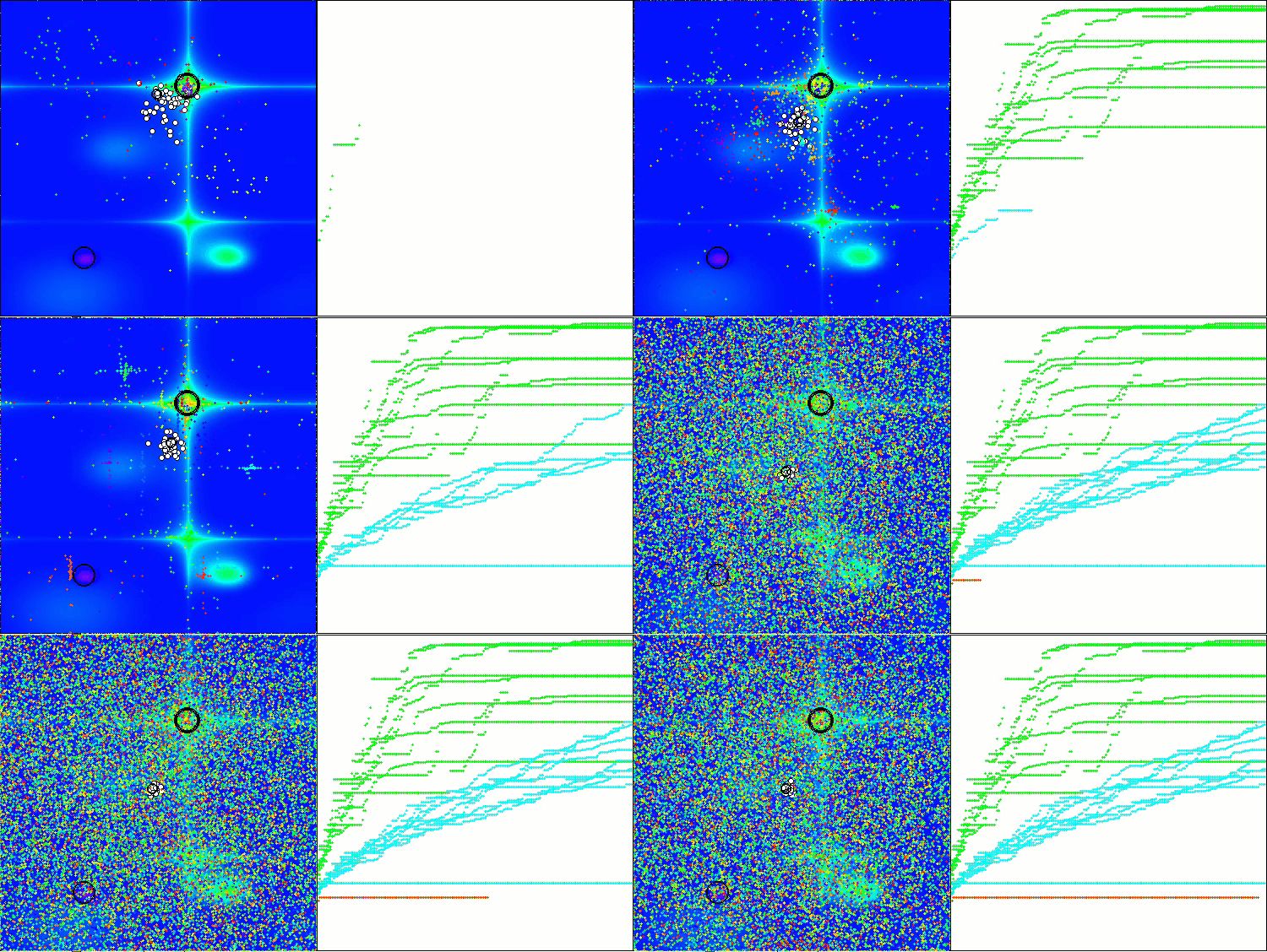
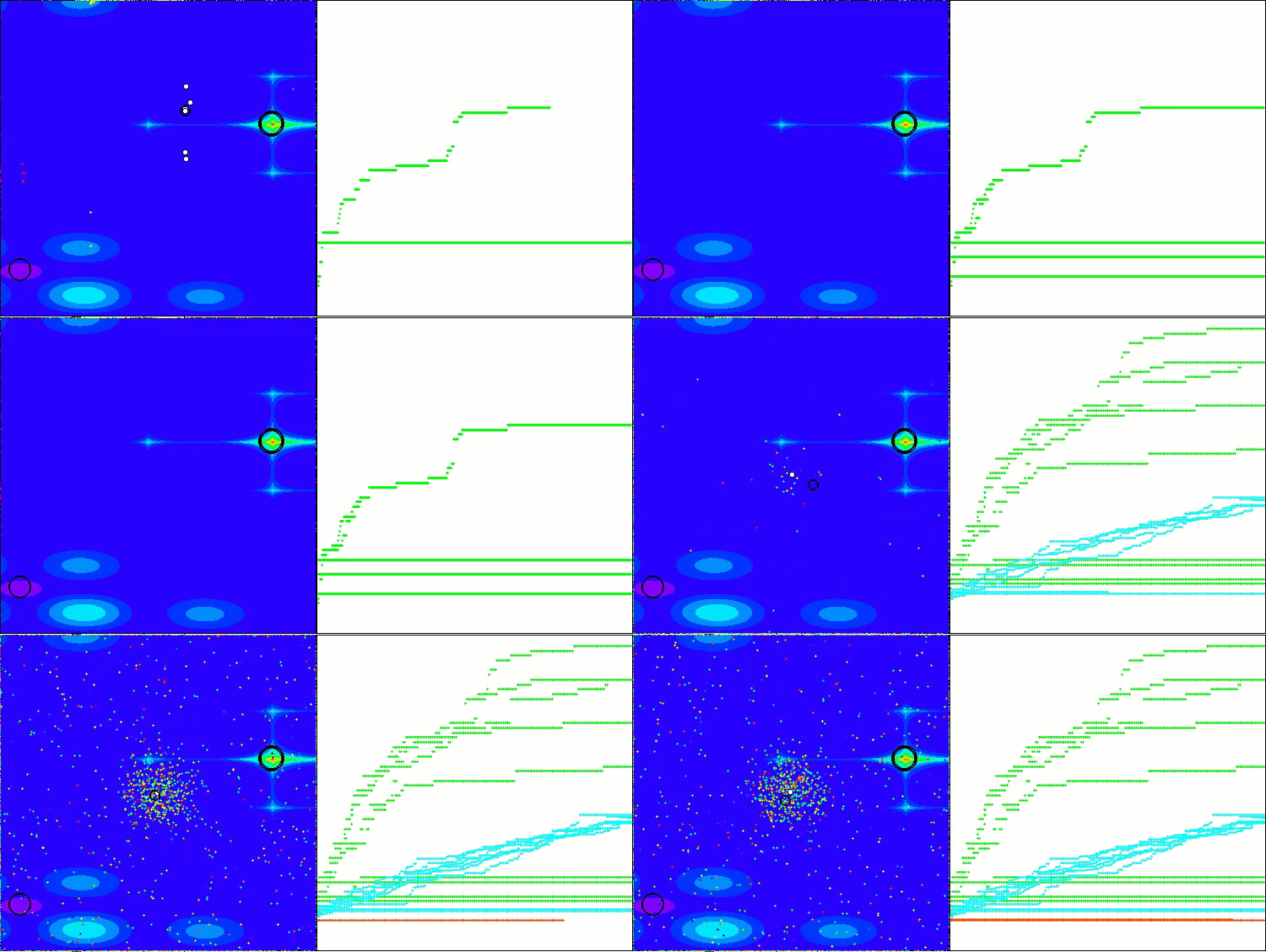
This time the results turned out to be much more promising and are already worthy of inclusion in the rating table, which will allow us to displace another outsider. The visualization shows a much more active movement of individuals in the population across the solution space. However, a new problem arose: there was a significant spread of results, and it was not possible to completely get rid of getting stuck in local optima.
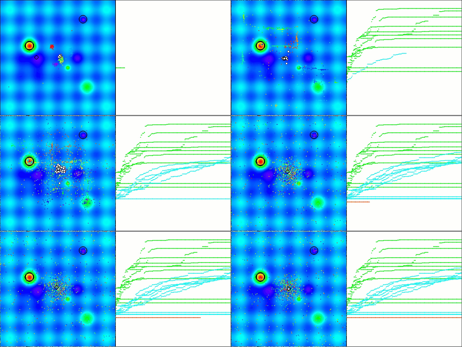
ATAm on the Hilly test functionality
ATAm on the Forest test function
ATAm on the Megacity test function
The artificial tribe algorithm is ranked 33rd in the ranking table.
| # | AO | Description | Hilly | Hilly final | Forest | Forest final | Megacity (discrete) | Megacity final | Final result | % of MAX | ||||||
| 10 p (5 F) | 50 p (25 F) | 1000 p (500 F) | 10 p (5 F) | 50 p (25 F) | 1000 p (500 F) | 10 p (5 F) | 50 p (25 F) | 1000 p (500 F) | ||||||||
| 1 | ANS | across neighbourhood search | 0.94948 | 0.84776 | 0.43857 | 2.23581 | 1.00000 | 0.92334 | 0.39988 | 2.32323 | 0.70923 | 0.63477 | 0.23091 | 1.57491 | 6.134 | 68.15 |
| 2 | CLA | code lock algorithm (joo) | 0.95345 | 0.87107 | 0.37590 | 2.20042 | 0.98942 | 0.91709 | 0.31642 | 2.22294 | 0.79692 | 0.69385 | 0.19303 | 1.68380 | 6.107 | 67.86 |
| 3 | AMOm | animal migration ptimization M | 0.90358 | 0.84317 | 0.46284 | 2.20959 | 0.99001 | 0.92436 | 0.46598 | 2.38034 | 0.56769 | 0.59132 | 0.23773 | 1.39675 | 5.987 | 66.52 |
| 4 | (P+O)ES | (P+O) evolution strategies | 0.92256 | 0.88101 | 0.40021 | 2.20379 | 0.97750 | 0.87490 | 0.31945 | 2.17185 | 0.67385 | 0.62985 | 0.18634 | 1.49003 | 5.866 | 65.17 |
| 5 | CTA | comet tail algorithm (joo) | 0.95346 | 0.86319 | 0.27770 | 2.09435 | 0.99794 | 0.85740 | 0.33949 | 2.19484 | 0.88769 | 0.56431 | 0.10512 | 1.55712 | 5.846 | 64.96 |
| 6 | SDSm | stochastic diffusion search M | 0.93066 | 0.85445 | 0.39476 | 2.17988 | 0.99983 | 0.89244 | 0.19619 | 2.08846 | 0.72333 | 0.61100 | 0.10670 | 1.44103 | 5.709 | 63.44 |
| 7 | AAm | archery algorithm M | 0.91744 | 0.70876 | 0.42160 | 2.04780 | 0.92527 | 0.75802 | 0.35328 | 2.03657 | 0.67385 | 0.55200 | 0.23738 | 1.46323 | 5.548 | 61.64 |
| 8 | ESG | evolution of social groups (joo) | 0.99906 | 0.79654 | 0.35056 | 2.14616 | 1.00000 | 0.82863 | 0.13102 | 1.95965 | 0.82333 | 0.55300 | 0.04725 | 1.42358 | 5.529 | 61.44 |
| 9 | SIA | simulated isotropic annealing (joo) | 0.95784 | 0.84264 | 0.41465 | 2.21513 | 0.98239 | 0.79586 | 0.20507 | 1.98332 | 0.68667 | 0.49300 | 0.09053 | 1.27020 | 5.469 | 60.76 |
| 10 | ACS | artificial cooperative search | 0.75547 | 0.74744 | 0.30407 | 1.80698 | 1.00000 | 0.88861 | 0.22413 | 2.11274 | 0.69077 | 0.48185 | 0.13322 | 1.30583 | 5.226 | 58.06 |
| 11 | ASO | anarchy society optimization | 0.84872 | 0.74646 | 0.31465 | 1.90983 | 0.96148 | 0.79150 | 0.23803 | 1.99101 | 0.57077 | 0.54062 | 0.16614 | 1.27752 | 5.178 | 57.54 |
| 12 | AOSm | atomic orbital search M | 0.80232 | 0.70449 | 0.31021 | 1.81702 | 0.85660 | 0.69451 | 0.21996 | 1.77107 | 0.74615 | 0.52862 | 0.14358 | 1.41835 | 5.006 | 55.63 |
| 13 | TSEA | turtle shell evolution algorithm (joo) | 0.96798 | 0.64480 | 0.29672 | 1.90949 | 0.99449 | 0.61981 | 0.22708 | 1.84139 | 0.69077 | 0.42646 | 0.13598 | 1.25322 | 5.004 | 55.60 |
| 14 | DE | differential evolution | 0.95044 | 0.61674 | 0.30308 | 1.87026 | 0.95317 | 0.78896 | 0.16652 | 1.90865 | 0.78667 | 0.36033 | 0.02953 | 1.17653 | 4.955 | 55.06 |
| 15 | CRO | chemical reaction optimization | 0.94629 | 0.66112 | 0.29853 | 1.90593 | 0.87906 | 0.58422 | 0.21146 | 1.67473 | 0.75846 | 0.42646 | 0.12686 | 1.31178 | 4.892 | 54.36 |
| 16 | BSA | bird swarm algorithm | 0.89306 | 0.64900 | 0.26250 | 1.80455 | 0.92420 | 0.71121 | 0.24939 | 1.88479 | 0.69385 | 0.32615 | 0.10012 | 1.12012 | 4.809 | 53.44 |
| 17 | HS | harmony search | 0.86509 | 0.68782 | 0.32527 | 1.87818 | 0.99999 | 0.68002 | 0.09590 | 1.77592 | 0.62000 | 0.42267 | 0.05458 | 1.09725 | 4.751 | 52.79 |
| 18 | SSG | saplings sowing and growing | 0.77839 | 0.64925 | 0.39543 | 1.82308 | 0.85973 | 0.62467 | 0.17429 | 1.65869 | 0.64667 | 0.44133 | 0.10598 | 1.19398 | 4.676 | 51.95 |
| 19 | BCOm | bacterial chemotaxis optimization M | 0.75953 | 0.62268 | 0.31483 | 1.69704 | 0.89378 | 0.61339 | 0.22542 | 1.73259 | 0.65385 | 0.42092 | 0.14435 | 1.21912 | 4.649 | 51.65 |
| 20 | ABO | african buffalo optimization | 0.83337 | 0.62247 | 0.29964 | 1.75548 | 0.92170 | 0.58618 | 0.19723 | 1.70511 | 0.61000 | 0.43154 | 0.13225 | 1.17378 | 4.634 | 51.49 |
| 21 | (PO)ES | (PO) evolution strategies | 0.79025 | 0.62647 | 0.42935 | 1.84606 | 0.87616 | 0.60943 | 0.19591 | 1.68151 | 0.59000 | 0.37933 | 0.11322 | 1.08255 | 4.610 | 51.22 |
| 22 | TSm | tabu search M | 0.87795 | 0.61431 | 0.29104 | 1.78330 | 0.92885 | 0.51844 | 0.19054 | 1.63783 | 0.61077 | 0.38215 | 0.12157 | 1.11449 | 4.536 | 50.40 |
| 23 | BSO | brain storm optimization | 0.93736 | 0.57616 | 0.29688 | 1.81041 | 0.93131 | 0.55866 | 0.23537 | 1.72534 | 0.55231 | 0.29077 | 0.11914 | 0.96222 | 4.498 | 49.98 |
| 24 | WOAm | wale optimization algorithm M | 0.84521 | 0.56298 | 0.26263 | 1.67081 | 0.93100 | 0.52278 | 0.16365 | 1.61743 | 0.66308 | 0.41138 | 0.11357 | 1.18803 | 4.476 | 49.74 |
| 25 | AEFA | artificial electric field algorithm | 0.87700 | 0.61753 | 0.25235 | 1.74688 | 0.92729 | 0.72698 | 0.18064 | 1.83490 | 0.66615 | 0.11631 | 0.09508 | 0.87754 | 4.459 | 49.55 |
| 26 | AEO | artificial ecosystem-based optimization algorithm | 0.91380 | 0.46713 | 0.26470 | 1.64563 | 0.90223 | 0.43705 | 0.21400 | 1.55327 | 0.66154 | 0.30800 | 0.28563 | 1.25517 | 4.454 | 49.49 |
| 27 | ACOm | ant colony optimization M | 0.88190 | 0.66127 | 0.30377 | 1.84693 | 0.85873 | 0.58680 | 0.15051 | 1.59604 | 0.59667 | 0.37333 | 0.02472 | 0.99472 | 4.438 | 49.31 |
| 28 | BFO-GA | bacterial foraging optimization - ga | 0.89150 | 0.55111 | 0.31529 | 1.75790 | 0.96982 | 0.39612 | 0.06305 | 1.42899 | 0.72667 | 0.27500 | 0.03525 | 1.03692 | 4.224 | 46.93 |
| 29 | SOA | simple optimization algorithm | 0.91520 | 0.46976 | 0.27089 | 1.65585 | 0.89675 | 0.37401 | 0.16984 | 1.44060 | 0.69538 | 0.28031 | 0.10852 | 1.08422 | 4.181 | 46.45 |
| 30 | ABHA | artificial bee hive algorithm | 0.84131 | 0.54227 | 0.26304 | 1.64663 | 0.87858 | 0.47779 | 0.17181 | 1.52818 | 0.50923 | 0.33877 | 0.10397 | 0.95197 | 4.127 | 45.85 |
| 31 | ACMO | atmospheric cloud model optimization | 0.90321 | 0.48546 | 0.30403 | 1.69270 | 0.80268 | 0.37857 | 0.19178 | 1.37303 | 0.62308 | 0.24400 | 0.10795 | 0.97503 | 4.041 | 44.90 |
| 32 | ADAMm | adaptive moment estimation M | 0.88635 | 0.44766 | 0.26613 | 1.60014 | 0.84497 | 0.38493 | 0.16889 | 1.39880 | 0.66154 | 0.27046 | 0.10594 | 1.03794 | 4.037 | 44.85 |
| 33 | ATAm | artificial tribe algorithm M | 0.71771 | 0.55304 | 0.25235 | 1.52310 | 0.82491 | 0.55904 | 0.20473 | 1.58867 | 0.44000 | 0.18615 | 0.09411 | 0.72026 | 3.832 | 42.58 |
| 34 | ASHA | artificial showering algorithm | 0.89686 | 0.40433 | 0.25617 | 1.55737 | 0.80360 | 0.35526 | 0.19160 | 1.35046 | 0.47692 | 0.18123 | 0.09774 | 0.75589 | 3.664 | 40.71 |
| 35 | ASBO | adaptive social behavior optimization | 0.76331 | 0.49253 | 0.32619 | 1.58202 | 0.79546 | 0.40035 | 0.26097 | 1.45677 | 0.26462 | 0.17169 | 0.18200 | 0.61831 | 3.657 | 40.63 |
| 36 | MEC | mind evolutionary computation | 0.69533 | 0.53376 | 0.32661 | 1.55569 | 0.72464 | 0.33036 | 0.07198 | 1.12698 | 0.52500 | 0.22000 | 0.04198 | 0.78698 | 3.470 | 38.55 |
| 37 | IWO | invasive weed optimization | 0.72679 | 0.52256 | 0.33123 | 1.58058 | 0.70756 | 0.33955 | 0.07484 | 1.12196 | 0.42333 | 0.23067 | 0.04617 | 0.70017 | 3.403 | 37.81 |
| 38 | Micro-AIS | micro artificial immune system | 0.79547 | 0.51922 | 0.30861 | 1.62330 | 0.72956 | 0.36879 | 0.09398 | 1.19233 | 0.37667 | 0.15867 | 0.02802 | 0.56335 | 3.379 | 37.54 |
| 39 | COAm | cuckoo optimization algorithm M | 0.75820 | 0.48652 | 0.31369 | 1.55841 | 0.74054 | 0.28051 | 0.05599 | 1.07704 | 0.50500 | 0.17467 | 0.03380 | 0.71347 | 3.349 | 37.21 |
| 40 | SDOm | spiral dynamics optimization M | 0.74601 | 0.44623 | 0.29687 | 1.48912 | 0.70204 | 0.34678 | 0.10944 | 1.15826 | 0.42833 | 0.16767 | 0.03663 | 0.63263 | 3.280 | 36.44 |
| 41 | NMm | Nelder-Mead method M | 0.73807 | 0.50598 | 0.31342 | 1.55747 | 0.63674 | 0.28302 | 0.08221 | 1.00197 | 0.44667 | 0.18667 | 0.04028 | 0.67362 | 3.233 | 35.92 |
| 42 | FAm | firefly algorithm M | 0.58634 | 0.47228 | 0.32276 | 1.38138 | 0.68467 | 0.37439 | 0.10908 | 1.16814 | 0.28667 | 0.16467 | 0.04722 | 0.49855 | 3.048 | 33.87 |
| 43 | GSA | gravitational search algorithm | 0.64757 | 0.49197 | 0.30062 | 1.44016 | 0.53962 | 0.36353 | 0.09945 | 1.00260 | 0.32667 | 0.12200 | 0.01917 | 0.46783 | 2.911 | 32.34 |
| 44 | BFO | bacterial foraging optimization | 0.61171 | 0.43270 | 0.31318 | 1.35759 | 0.54410 | 0.21511 | 0.05676 | 0.81597 | 0.42167 | 0.13800 | 0.03195 | 0.59162 | 2.765 | 30.72 |
| 45 | ABC | artificial bee colony | 0.63377 | 0.42402 | 0.30892 | 1.36671 | 0.55103 | 0.21874 | 0.05623 | 0.82600 | 0.34000 | 0.14200 | 0.03102 | 0.51302 | 2.706 | 30.06 |
Summary
In this article, we have examined in detail one of the most modern optimization algorithms – the ATA algorithm. Although this algorithm does not perform exceptionally well compared to other methods, it makes a valuable contribution to our understanding of dynamic population state management and methods for analyzing problems associated with local optima.
Interest in the ATA algorithm is not limited to its two main phases, which in themselves are of little value as solution methods. Much more important is the approach that uses dynamic selection of the movement phases of individuals and control over the state of the population. It is this aspect that allows us to more effectively adapt the algorithm to changing problem conditions and improve the quality of the solutions obtained. Thus, the study of ATA opens new horizons for further research in the field of algorithmic optimization and can serve as a basis for the development of more advanced methods.
I am also sure that various operators can be applied to the algorithm under discussion, which will significantly increase its efficiency. For example, using selection operators based on sorting or crossover can significantly improve results.
However, it is worth noting that the current version of the algorithm does not have any dependencies on the quality of the solution, and also lacks combinatorial properties, which limits its capabilities. All of these aspects represent interesting directions for further research and improvement, although they are beyond the scope of this article. I would be very happy if any of the readers decide to experiment with the proposed changes and share their versions of the algorithm in the comments.
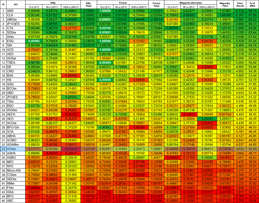
Figure 3. Color gradation of algorithms according to relevant tests Results greater than or equal to 0.99 are highlighted in white
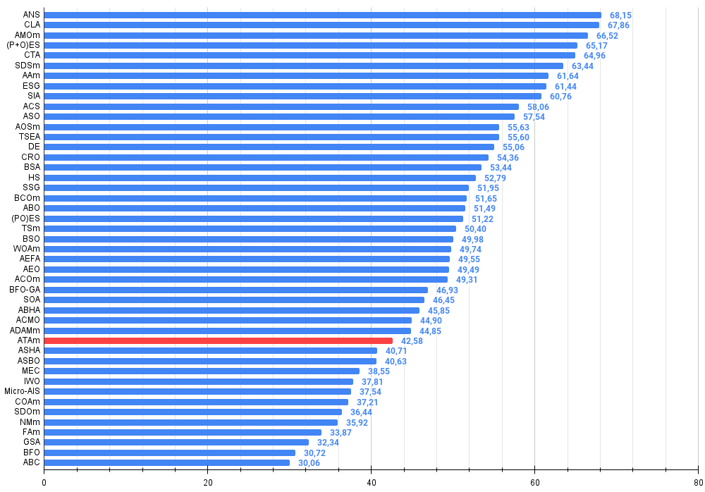
Figure 4. Histogram of algorithm testing results (scale from 0 to 100, the higher the better, where 100 is the maximum possible theoretical result, in the archive there is a script for calculating the rating table)
ATAm pros and cons:
Pros:
- Small number of external parameters.
- Simple implementation.
- Interesting idea of dynamically switching search strategies.
Cons:
- High scatter of results.
- Low convergence accuracy.
- Tendency to get stuck.
The article is accompanied by an archive with the current versions of the algorithm codes. The author of the article is not responsible for the absolute accuracy in the description of canonical algorithms. Changes have been made to many of them to improve search capabilities. The conclusions and judgments presented in the articles are based on the results of the experiments.
Programs used in the article
| # | Name | Type | Description |
|---|---|---|---|
| 1 | #C_AO.mqh | Include | Parent class of population optimization algorithms |
| 2 | #C_AO_enum.mqh | Include | Enumeration of population optimization algorithms |
| 3 | TestFunctions.mqh | Include | Library of test functions |
| 4 | TestStandFunctions.mqh | Include | Test stand function library |
| 5 | Utilities.mqh | Include | Library of auxiliary functions |
| 6 | CalculationTestResults.mqh | Include | Script for calculating results in the comparison table |
| 7 | Testing AOs.mq5 | Script | The unified test stand for all population optimization algorithms |
| 8 | Simple use of population optimization algorithms.mq5 | Script | A simple example of using population optimization algorithms without visualization |
| 9 | Test_AO_ATAm.mq5 | Script | ATAm test stand |
Translated from Russian by MetaQuotes Ltd.
Original article: https://www.mql5.com/ru/articles/16588
Warning: All rights to these materials are reserved by MetaQuotes Ltd. Copying or reprinting of these materials in whole or in part is prohibited.
This article was written by a user of the site and reflects their personal views. MetaQuotes Ltd is not responsible for the accuracy of the information presented, nor for any consequences resulting from the use of the solutions, strategies or recommendations described.
 Neural Networks in Trading: A Multi-Agent Self-Adaptive Model (MASA)
 Analyzing binary code of prices on the exchange (Part I): A new look at technical analysis
 Analyzing binary code of prices on the exchange (Part II): Converting to BIP39 and writing GPT model
 Self Optimizing Expert Advisors in MQL5 (Part 13): A Gentle Introduction To Control Theory Using Matrix Factorization
- Free trading apps
- Over 8,000 signals for copying
- Economic news for exploring financial markets
You agree to website policy and terms of use