Big Bang - Big Crunch (BBBC) algorithm

Contents

1. Introduction
2. Implementation of the algorithm
3. Test results

Introduction

In the vast expanses of the Universe, where stars are born and die, there are hidden secrets that humanity strives to unravel. Big Bang-Big Crunch (BBBC) method is a global optimization algorithm inspired by processes occurring in space. Let's explore this fascinating concept.

The Big Bang and Crunch Theory was proposed as an alternative scenario for the end of the Universe by physicists Alexander Friedmann and Georges Lemaitre in the early 20th century. They noticed that Einstein's equations of general relativity allow for both expansion and contraction of the universe. Friedman proved mathematically that the Universe cannot remain static and must either expand or contract. He identified three possible scenarios for its development: eternal expansion, expansion followed by contraction, and an oscillatory regime.

Throughout the 20th century, many scientists developed ideas that combined the Big Bang and Big Crunch into a cyclical model. Today, the Big Crunch theory is not the main cosmological model, since observations show that the Universe is expanding at an accelerating rate. However, this concept is an interesting idea that suggests a cyclical nature of the Universe evolution. Main stages:

• The Big Bang, when the initial state of high density and temperature passes into a stage of rapid expansion and dissipation of energy with the formation of matter and space-time, and a chaotic distribution of particles.
• The Big Crunch, when gravitational forces stop the expansion and contraction begins, all matter is pulled back into a point, returning to a state of high density.
• The cyclicity is expressed in the sequence of a new Big Bang after a Big Crunch, the process can be repeated infinitely, and each cycle can have different physical constants.

The Big Bang-Big Crunch algorithm was proposed in 2006 by scientists Osman K. Erol and Ibrahim Eksin of Istanbul Technical University, Turkey.

Implementation of the algorithm

Just as in the Big Bang theory, where the Universe begins its existence with a powerful burst of energy, so in the BBBC method we observe an initial phase full of randomness and diversity. In the Big Bang phase, a population of random dots is created. Each of them represents a candidate for a solution. These dots are scattered across the vast search space, ready to be explored, but once chaos finds its place, the Big Crunch phase begins. The dots tend to move towards the "center of mass", just as galaxies are attracted to each other through gravity. This moment is the culmination, when all efforts come together in search of the optimal solution. 

Here are the stages of the algorithm, the path from chaos to order:

1. Big Bang phase. In this first step, an initial population of N random points is created. Each point occupies its own place in space, evenly distributed within the given boundaries.

2. Big Crunch phase. Transition to calculating the "center of mass" — the dot all others strive to. Using the equation (Fig. 1), find the coordinates of the center, which will become the new beginning for the next steps.

3. Generating new dots. New points begin to exist around the center of mass. They are formed with a normal distribution, following an equation that gives them the direction and magnitude of movement.

The BBBC method seeks harmony between exploration and refinement. With each new generation, the spread of points during generation decreases, which allows the algorithm to refine the optimal solution found.

Just as in space, where every move matters, in the world of optimization, every calculation brings us closer to our goal. By immersing ourselves in this method, we not only open new horizons, but also become part of a great cosmic process in search of a better solution.

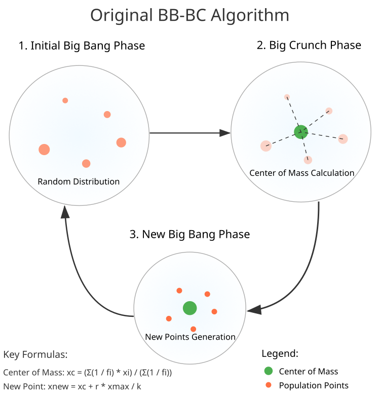
Figure 1. BBBC algorithm structure

Let's write a pseudocode of the BBBC algorithm:

    Increase epochNow

    // Initialization (Big Bang)
    if revision == false
        For each i individual from 0 to popSize-1
            For each c coordinate from 0 to coords-1
                New coordinate = Generate random number (rangeMin[c], rangeMax[c])
        Set 'revision' to 'true'
        Return

    // Big Crunch Phase
    If epochNow % bigBangPeriod != 0
        For each c coordinate from 0 to coords-1
            numerator = 0, denominator = 0
            For each i individual from 0 to popSize-1
                fitness = Maximum (Absolute value (a [i].f), 1e-10)
                вес = 1.0 / fitness
                numerator += weight * dot coordinate
                denominator += weight
            centerMass [c] = (denominator > 1e-10) ? numerator / denominator : cB [c]

        For each i individual from 0 to popSize-1
            For each c coordinate from 0 to coords-1
                r = Generate a normal random number (0, -1.0, 1.0, 1)
                 New coordinate = centerMass [c] + r * rangeMax [c] / epochNow
    // Big Bang phase
    Otherwise
        For each i individual from 0 to popSize-1
            For each c coordinate from 0 to coords-1
                New coordinate = Generate normal random number (cB [c], rangeMin [c], rangeMax [c], standard deviation = 8)

   Repeat until the the Big Crunch phase stop criterion is met

Let's move on to writing the code. Let's write the definition of the C_AO_BBBC class, a descendant of C_AO:

Public methods:

• Constructor and destructor
• SetParams () — set parameters (population size and periodicity of the Big Bang)
• Init () — initialization of the algorithm with given search boundaries
• Moving () — main method implementing the Big Bang and Big Crunch phases
• Revision () — method of updating the best found solution

Private fields:

• epochs — total number of epochs of the algorithm operation
• epochNow — current era
• centerMass [] — array for storing the coordinates of the center of mass
  

The class is an implementation of the BBBC algorithm, where all the main calculations occur in the Moving() and Revision() methods, and the necessary population data is stored in the C_AO base class.

//——————————————————————————————————————————————————————————————————————————————
class C_AO_BBBC : public C_AO
{
  public: //--------------------------------------------------------------------
  ~C_AO_BBBC () { }
  C_AO_BBBC ()
  {
    ao_name = "BBBC";
    ao_desc = "Big Bang - Big Crunch Algorithm";
    ao_link = "https://www.mql5.com/en/articles/16701";

    popSize       = 50;
    bigBangPeriod = 3;

    ArrayResize (params, 2);
    params [0].name = "popSize";       params [0].val = popSize;
    params [1].name = "bigBangPeriod"; params [1].val = bigBangPeriod;
  }

  void SetParams ()
  {
    popSize       = (int)params [0].val;
    bigBangPeriod = (int)params [1].val;
  }

  bool Init (const double &rangeMinP  [],  // minimum search range
             const double &rangeMaxP  [],  // maximum search range
             const double &rangeStepP [],  // search step
             const int epochsP = 0);       // number of epochs

  void Moving   ();
  void Revision ();

  //----------------------------------------------------------------------------
  int bigBangPeriod;       // Big Bang periodicity

  private: //-------------------------------------------------------------------
  int epochs;              // total number of epochs
  int epochNow;            // current epoch
  double centerMass [];    // center of mass
};
//——————————————————————————————————————————————————————————————————————————————

Init method of the C_AO_BBBC class:

The method initializes the algorithm and takes the following parameters:

• rangeMinP [] — array of minimum values for each coordinate
• rangeMaxP [] — array of maximum values for each coordinate
• rangeStepP [] — array of discretization steps for each coordinate
• epochsP — number of algorithm operation epochs (default 0)

Method actions:

1. Calls StandardInit () of the base class for initializing common parameters
2. Sets the total number of epochs (epochs) and resets the current epoch counter (epochNow)
3. Allocates memory for the center of mass array (centerMass) of coords (number of coordinates) size

//——————————————————————————————————————————————————————————————————————————————
bool C_AO_BBBC::Init (const double &rangeMinP  [],
                      const double &rangeMaxP  [],
                      const double &rangeStepP [],
                      const int epochsP = 0)
{
  // Initialize the base class
  if (!StandardInit (rangeMinP, rangeMaxP, rangeStepP)) return false;

  //----------------------------------------------------------------------------
  epochs   = epochsP;
  epochNow = 0;

  // Allocate memory for arrays
  ArrayResize (centerMass, coords);

  return true;
}
//——————————————————————————————————————————————————————————————————————————————

The Moving method of the BB-BC algorithm consists of three main parts:

1. Starting initialization (if revision = false):

• Create an initial population of random points
• Bring them to a discrete search grid

2. Big Crunch phase (if 'epoch' is not a multiple of bigBangPeriod):

• Calculate the center of mass using the equation: xc = (Σ(1/fi)*xi) / (Σ(1/fi))
• Generate new points around the center of mass using the equation: xnew = xc + r * xmax / epoch
• Use normal distribution for random numbers

3. Big Bang phase (if 'epoch' is a multiple of bigBangPeriod):

• Generate new dots using normal distribution
• Use the best solution as the average
• Use deviation = 8 for broad search

All new dots are limited by the specified search boundaries and are converted to a discrete grid.

//——————————————————————————————————————————————————————————————————————————————
void C_AO_BBBC::Moving ()
{
  epochNow++;

  // Starting initialization (Big Bang)
  if (!revision)
  {
    for (int i = 0; i < popSize; i++)
    {
      for (int c = 0; c < coords; c++)
      {
        // Generate random starting dots
        a [i].c [c] = u.RNDfromCI (rangeMin [c], rangeMax [c]);
        // Reduction to discrete search grid
        a [i].c [c] = u.SeInDiSp (a [i].c [c], rangeMin [c], rangeMax [c], rangeStep [c]);
      }
    }
    revision = true;
    return;
  }

  //----------------------------------------------------------------------------
  // Big Crunch phase - big collapse
  if (epochNow % bigBangPeriod != 0)
  {
    for (int c = 0; c < coords; c++)
    {
      double numerator = 0;
      double denominator = 0;

      for (int i = 0; i < popSize; i++)
      {
        // Calculate weight as the inverse of the fitness function value
        double fitness = MathMax (MathAbs (a [i].f), 1e-10);
        double weight = 1.0 / fitness;

        // Summation to calculate the center of mass using the equation
        // xc = (Σ(1/fi)xi) / (Σ(1/fi))
        numerator += weight * a [i].c [c];
        denominator += weight;
      }

      // Determine the coordinates of the center of mass
      centerMass [c] = denominator > 1e-10 ? numerator / denominator : cB [c];
    }

    for (int i = 0; i < popSize; i++)
    {
      for (int c = 0; c < coords; c++)
      {
        double r = u.GaussDistribution (0, -1.0, 1.0, 1);

        // Generate a new point using the equation
        // xnew = xc + r*xmax/k
        double newPoint = centerMass [c] + r * rangeMax [c] / epochNow;

        // Constrain within the allowed area and convert to grid
        a [i].c [c] = u.SeInDiSp (newPoint, rangeMin [c], rangeMax [c], rangeStep [c]);
      }
    }
  }
  //----------------------------------------------------------------------------
  // Big Bang phase - big bang
  else
  {
    for (int i = 0; i < popSize; i++)
    {
      for (int c = 0; c < coords; c++)
      {
        a [i].c [c] = u.GaussDistribution (cB [c], rangeMin [c], rangeMax [c], 8);
        a [i].c [c] = u.SeInDiSp (a [i].c [c], rangeMin [c], rangeMax [c], rangeStep [c]);
      }
    }
  }
}
//——————————————————————————————————————————————————————————————————————————————

The Revision method performs two main functions:

Find the best solution:

• Initialize the index of the best solution (bestInd = -1)
• Iterate over all points in the population
• If a better solution than the current one is found:
  • Updates the value of the best fitness function (fB)
  • Save the index of the best solution (bestInd)

Best solution update:

• If a better solution is found (bestInd != -1):
  • Copies all coordinates of the best solution from the array to the cB best solution array
    

The method provides updating information about the globally best solution found for the entire duration of the algorithm operation.

//——————————————————————————————————————————————————————————————————————————————
void C_AO_BBBC::Revision ()
{
  int bestInd = -1;

  // Find the best solution in the current population
  for (int i = 0; i < popSize; i++)
  {
    if (a [i].f > fB)
    {
      fB = a [i].f;
      bestInd = i;
    }
  }

  // Update the best known solution
  if (bestInd != -1) ArrayCopy (cB, a [bestInd].c, 0, 0, WHOLE_ARRAY);
}
//——————————————————————————————————————————————————————————————————————————————

The authors of the BBBC algorithm claim that it is capable of competing with well-known strong algorithms, such as genetic algorithms (GAs), outperforming them in significantly fewer epochs.

As evidence, they cite test results on standard and widely used synthetic benchmarks, such as the sphere (also known as paraboloid or ellipsoid), Ackley, and Rastrigin. Let's take a look at a visualization of the algorithm performance on two of these benchmarks.

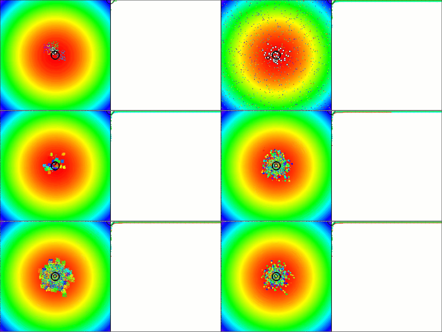
  BBBC on the Paraboloid test function

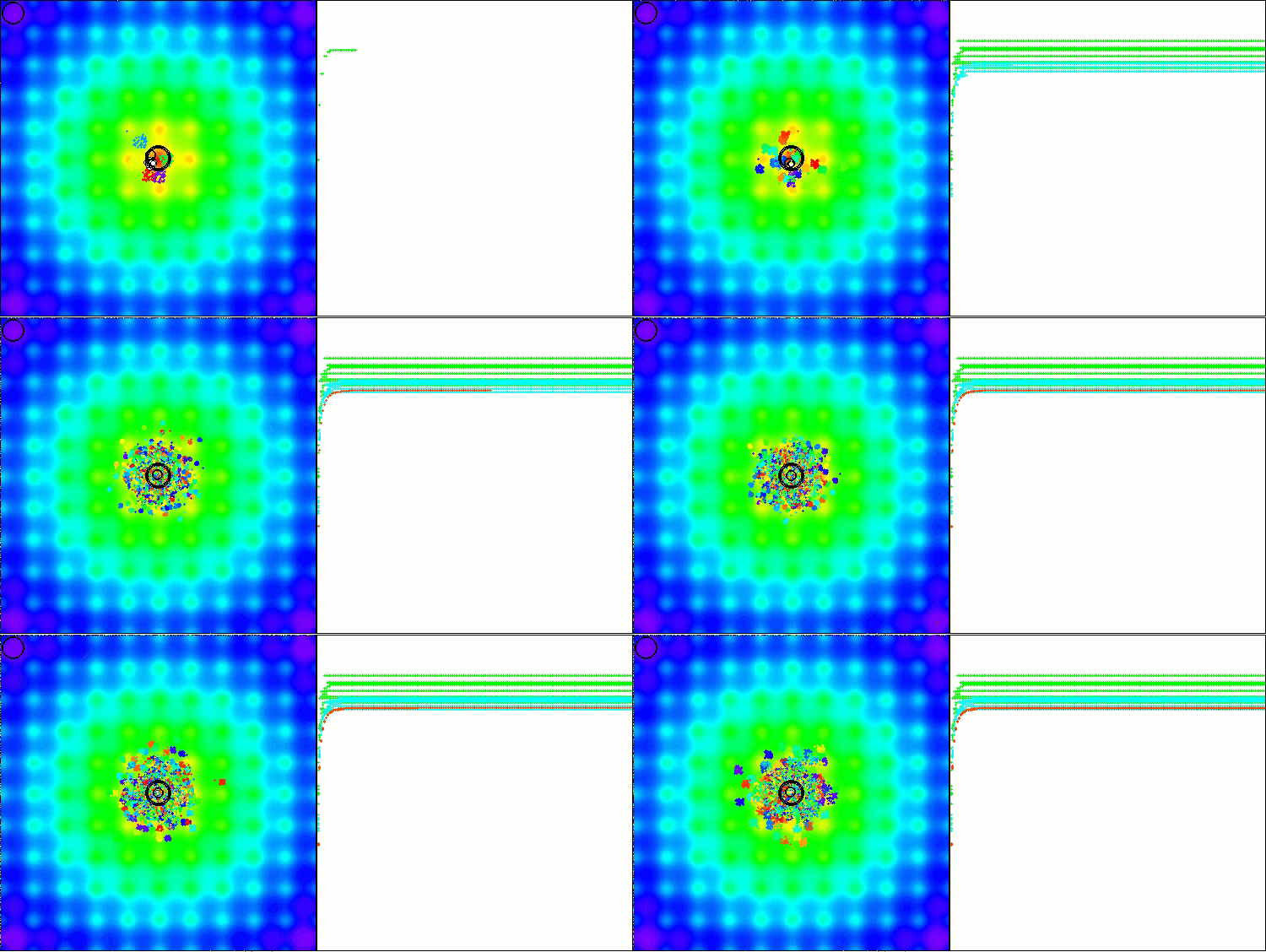
BBBC on the Ackley test function

Indeed, the results are impressive. It is particularly noteworthy that the results for high-dimensional problems (red line) differ little from the results for low-dimensional problems (green line), indicating the high scalability of the algorithm. Although the convergence accuracy on the Ackley function is not perfect, the results are still noteworthy.

Now let's look at the results of BBBC's work on our test functions specially developed for optimization algorithms.

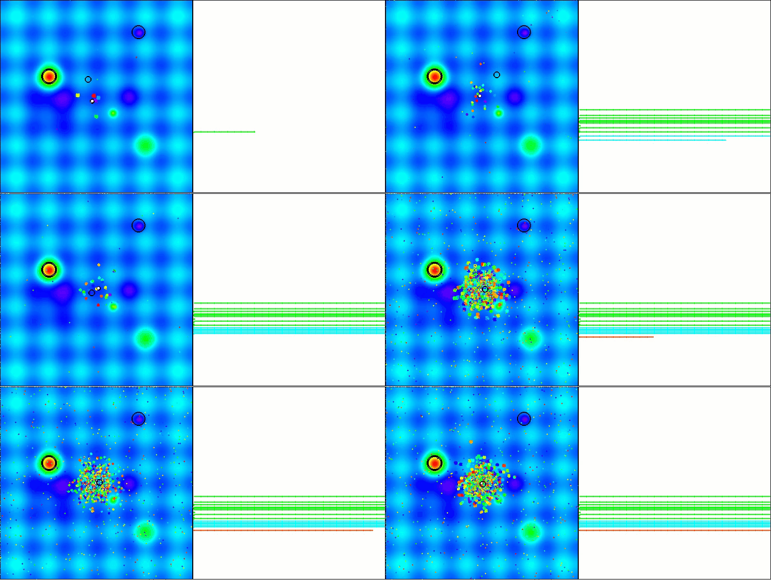
BBBC on the Hilly test function

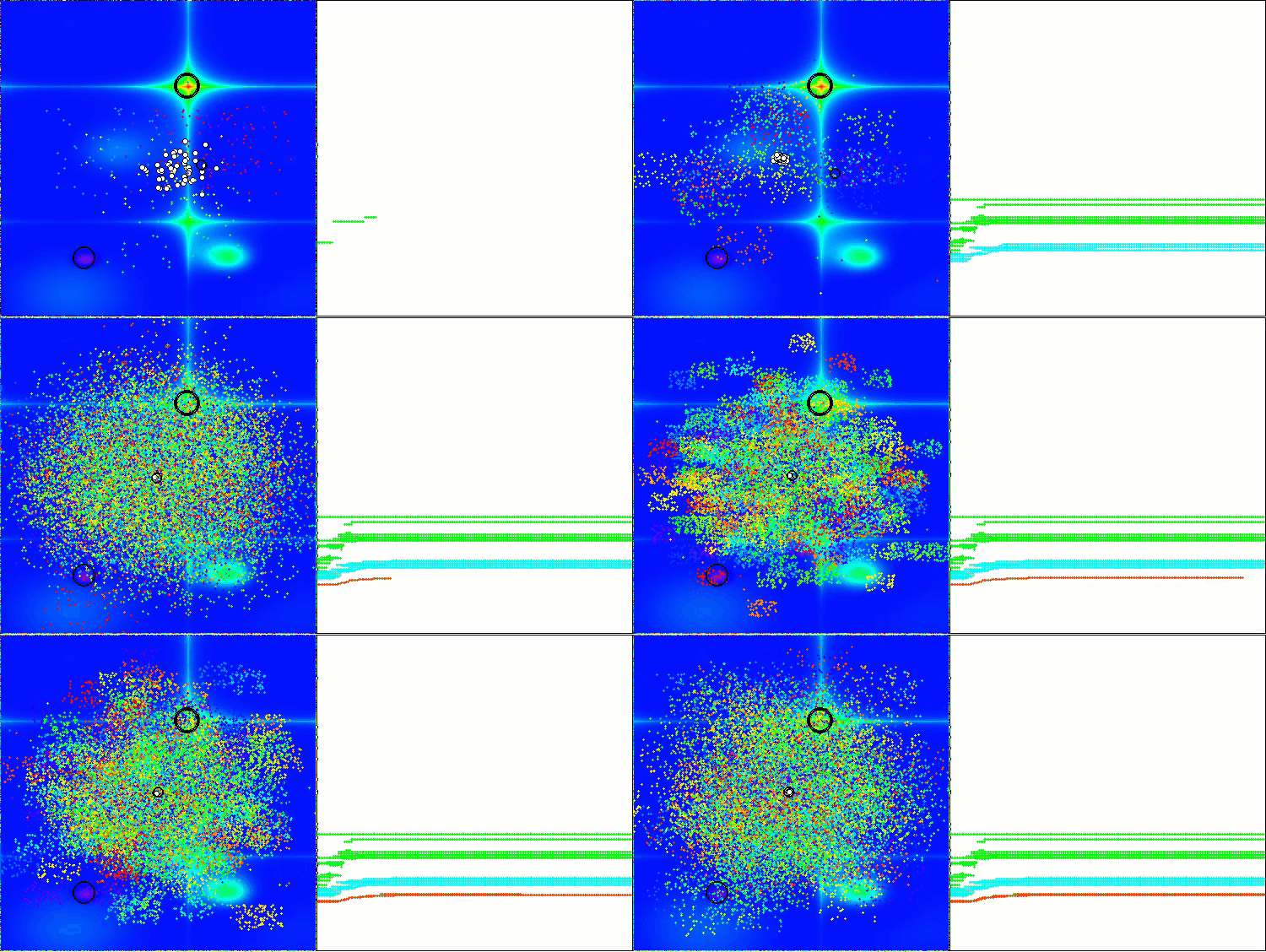
  BBBC on the Forest test function

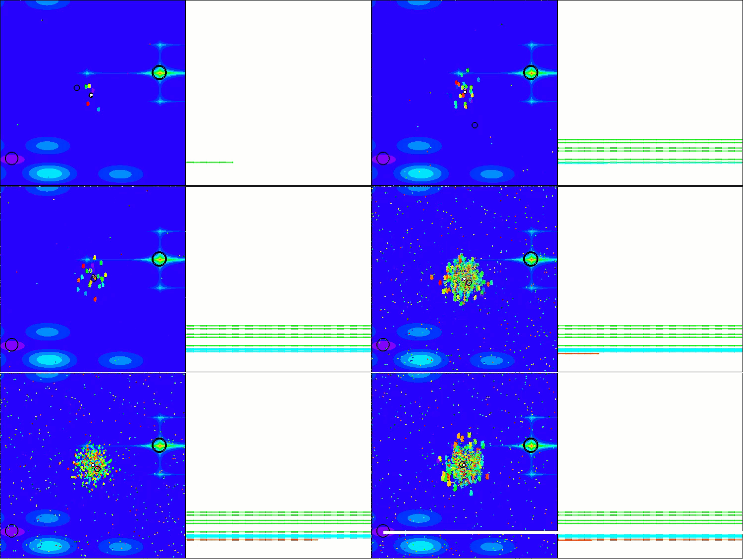
  BBBC on the Megacity test function

Unfortunately, the algorithm's magic stopped working on our benchmarks. What is the reason? First of all, it is worth paying attention to the fact that, as in the case of the previous functions, the algorithm population focuses its "attention" on the central part of the search space on the Hilly, Forest and Megacity tests. This observation raises certain questions and seems rather strange.

Let's take a look under the hood of the BBBC algorithm and examine its inner workings. We will see that when using the "center of mass", the dots distributed throughout space tend to collapse into the middle of the function's range. This happens because the center of mass of the dots is exactly in the center, which creates the illusion of the algorithm efficiency. This coincidence leads to the algorithm being able to successfully find optima for sphere-like functions (with the global optimum at the center of the range). However, in reality, this is not the result of the algorithm's outstanding search capabilities, but a lucky coincidence. For example, if the algorithm started at coordinate 0.0, it would ideally reach the global optimum on the first iteration.

It should be noted that most standard test functions widely used to evaluate various algorithms have a global optimum located in the center of the search space. Such tests may not always be reliable, and for some algorithms, such as BBBC, they can be misleading about the actual search capabilities of the algorithm.

To avoid false positive results during testing, I have developed special test functions that:

1. are not symmetrical
2. have a global optimum that is not located in the center of the search space
3. are not periodic 
4. have a small proportion of the surface located above the midline in height. 

These characteristics help reduce the probability of accidentally hitting the global optimum and provide a more objective assessment of the efficiency of optimization algorithms.

Now let's take a look at the printout of BBBC's results on the test functions collected in the table below. It is very important.

Big Bang on every 2nd epoch	Big Bang on every 3rd epoch	Big Bang on every 10th epoch
BBBC|Big Bang - Big Crunch Algorithm|50.0|2.0| ============================= 5 Hilly's; Func runs: 10000; result: 0.5789409521562645 25 Hilly's; Func runs: 10000; result: 0.36005433010965165 500 Hilly's; Func runs: 10000; result: 0.25650127842145554 ============================= 5 Forest's; Func runs: 10000; result: 0.5232991213500953 25 Forest's; Func runs: 10000; result: 0.293874681679014 500 Forest's; Func runs: 10000; result: 0.18830469994313143 ============================= 5 Megacity's; Func runs: 10000; result: 0.3269230769230769 25 Megacity's; Func runs: 10000; result: 0.15584615384615388 500 Megacity's; Func runs: 10000; result: 0.09743846153846236 ============================= All score: 2.78118 (30.90%)	BBBC|Big Bang - Big Crunch Algorithm|50.0|3.0| ============================= 5 Hilly's; Func runs: 10000; result: 0.5550785088841808 25 Hilly's; Func runs: 10000; result: 0.3605042956384694 500 Hilly's; Func runs: 10000; result: 0.25635343911025843 ============================= 5 Forest's; Func runs: 10000; result: 0.48703749499939086 25 Forest's; Func runs: 10000; result: 0.2897958021406425 500 Forest's; Func runs: 10000; result: 0.1865439156477803 ============================= 5 Megacity's; Func runs: 10000; result: 0.28307692307692306 25 Megacity's; Func runs: 10000; result: 0.15692307692307694 500 Megacity's; Func runs: 10000; result: 0.09701538461538546 ============================= All score: 2.67233 (29.69%)	BBBC|Big Bang - Big Crunch Algorithm|50.0|10.0| ============================= 5 Hilly's; Func runs: 10000; result: 0.4883607839451155 25 Hilly's; Func runs: 10000; result: 0.3344059754605514 500 Hilly's; Func runs: 10000; result: 0.25564528470980497 ============================= 5 Forest's; Func runs: 10000; result: 0.492293124748422 25 Forest's; Func runs: 10000; result: 0.28653857694657936 500 Forest's; Func runs: 10000; result: 0.1844110334128521 ============================= 5 Megacity's; Func runs: 10000; result: 0.3230769230769231 25 Megacity's; Func runs: 10000; result: 0.15261538461538465 500 Megacity's; Func runs: 10000; result: 0.09653846153846235 ============================= All score: 2.61389 (29.04%)

Please note that the test results show minor differences from each other and are within the natural range of values. This indicates the weak search capabilities of the strategy used, which in essence differs little from random search. In this regard, it is appropriate to present the results of testing the random walk (RW) algorithm. This algorithm was mentioned in previous articles, but the results of its operation were not presented. Now it is time to do it.

The presentation of the results of the RW algorithm is necessary in order to evaluate how much more efficient various search strategies are compared to simple random scattering of points in space. Below is the average result for 100 runs on test functions (usually I do 10).

RW|Random Walk|50.0|
=============================
5 Hilly's; Func runs: 10000; result: 0.48753502068617777
25 Hilly's; Func runs: 10000; result: 0.3215913699940513
500 Hilly's; Func runs: 10000; result: 0.2578113480890265
=============================
5 Forest's; Func runs: 10000; result: 0.3755402348403822
25 Forest's; Func runs: 10000; result: 0.21943566240362317
500 Forest's; Func runs: 10000; result: 0.15877419882827945
=============================
5 Megacity's; Func runs: 10000; result: 0.27969230769230796
25 Megacity's; Func runs: 10000; result: 0.14916923076923083
500 Megacity's; Func runs: 10000; result: 0.098473846153847
=============================
All score: 2.34802 (26.09%)

I will provide the code of the RW algorithm. It is very simple. As usual, the Moving function is responsible for updating the coordinates of each individual in the population. For each individual, it generates random values in a given range and then adjusts them using the SeInDiSp function to match the step change.

//——————————————————————————————————————————————————————————————————————————————
void C_AO_RW::Moving ()
{
  for (int w = 0; w < popSize; w++)
  {
    for (int c = 0; c < coords; c++)
    {
      a [w].c [c] = u.RNDfromCI (rangeMin [c], rangeMax [c]);
      a [w].c [c] = u.SeInDiSp  (a [w].c [c], rangeMin [c], rangeMax [c], rangeStep [c]);
    }
  }
}
//——————————————————————————————————————————————————————————————————————————————

The Revision function checks all individuals in the population to find the individual with the best fitness function (fB). If such an individual is found, its coordinates are copied into the global best score (cB).

//——————————————————————————————————————————————————————————————————————————————
void C_AO_RW::Revision ()
{
  int ind = -1;

  for (int i = 0; i < popSize; i++)
  {
    if (a [i].f > fB)
    {
      fB = a [i].f;
      ind = i;
    }
  }

  if (ind != -1) ArrayCopy (cB, a [ind].c, 0, 0, WHOLE_ARRAY);
}
//——————————————————————————————————————————————————————————————————————————————

Now we will make some changes to the original BBBC algorithm to neutralize its illusory advantages on problems with a global optimum in the center of the range of parameters being optimized and to allow objective tests. Let's look at the differences in the code. Changes were made to the Moving method:

1. Removed the center of mass calculation
2. Changed Big Bang phase:

• Instead of the center of mass (centerMass), the best solution (cB) is used
• Use the equation: xnew = cB + r*range/epochNow ("range" is now the difference between "rangeMax" and "rangeMin")
  

//——————————————————————————————————————————————————————————————————————————————
void C_AO_BBBC::Moving ()
{
  epochNow++;

  // Starting initialization (Big Bang)
  if (!revision)
  {
    for (int i = 0; i < popSize; i++)
    {
      for (int c = 0; c < coords; c++)
      {
        // Generate random starting dots
        a [i].c [c] = u.RNDfromCI (rangeMin [c], rangeMax [c]);
        // Reduction to discrete search grid
        a [i].c [c] = u.SeInDiSp (a [i].c [c], rangeMin [c], rangeMax [c], rangeStep [c]);
      }
    }
    revision = true;
    return;
  }

  //--------------------------------------------------------------------------
  for (int i = 0; i < popSize; i++)
  {
    //Big Crunch phase - big collapse
    if (epochNow % bigBangPeriod != 0)
    {
      for (int c = 0; c < coords; c++)
      {
        // Calculate the size of the search space for the current coordinate
        double range = rangeMax [c] - rangeMin [c];

        // Generate a random number in the range [-1, 1]
        double r = u.GaussDistribution (0, -1.0, 1.0, 1);

        // Generate a new point using the equation
        // xnew = xc + r*(xmax - xmin)/(k)
        double newPoint = cB [c] + r * range / epochNow;

        // Constrain within the allowed area and convert to grid
        a [i].c [c] = u.SeInDiSp (newPoint, rangeMin [c], rangeMax [c], rangeStep [c]);
      }
    }
    // Big Bang phase - big bang
    else
    {
      for (int c = 0; c < coords; c++)
      {
        a [i].c [c] = u.GaussDistribution (cB [c], rangeMin [c], rangeMax [c], 8);
        a [i].c [c] = u.SeInDiSp (a [i].c [c], rangeMin [c], rangeMax [c], rangeStep [c]);
      }
    }
  }
}
//——————————————————————————————————————————————————————————————————————————————

Test results

Results of the adjusted BBBC algorithm:

BBBC|Big Bang-Big Crunch Algorithm|50.0|
=============================
5 Hilly's; Func runs: 10000; result: 0.6053080737014771
25 Hilly's; Func runs: 10000; result: 0.45249601882946056
500 Hilly's; Func runs: 10000; result: 0.31255376970202864
=============================
5 Forest's; Func runs: 10000; result: 0.5232283922331299
25 Forest's; Func runs: 10000; result: 0.354256711141388
500 Forest's; Func runs: 10000; result: 0.20417356281490023
=============================
5 Megacity's; Func runs: 10000; result: 0.3976923076923077
25 Megacity's; Func runs: 10000; result: 0.19430769230769235
500 Megacity's; Func runs: 10000; result: 0.11286153846153954
=============================
All score: 3.15688 (35.08%)

Now the test results objectively reflect the capabilities of the BBBC algorithm. The visualization shows the formation of the same "stars" as in the original algorithm, but now the search occurs in real promising areas, and not just predominantly in the center of the search space.

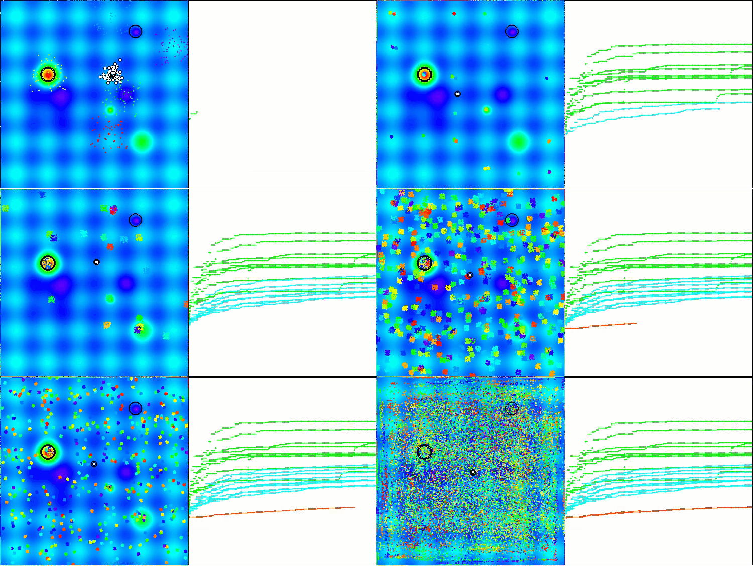
BHAm on the Hilly test function

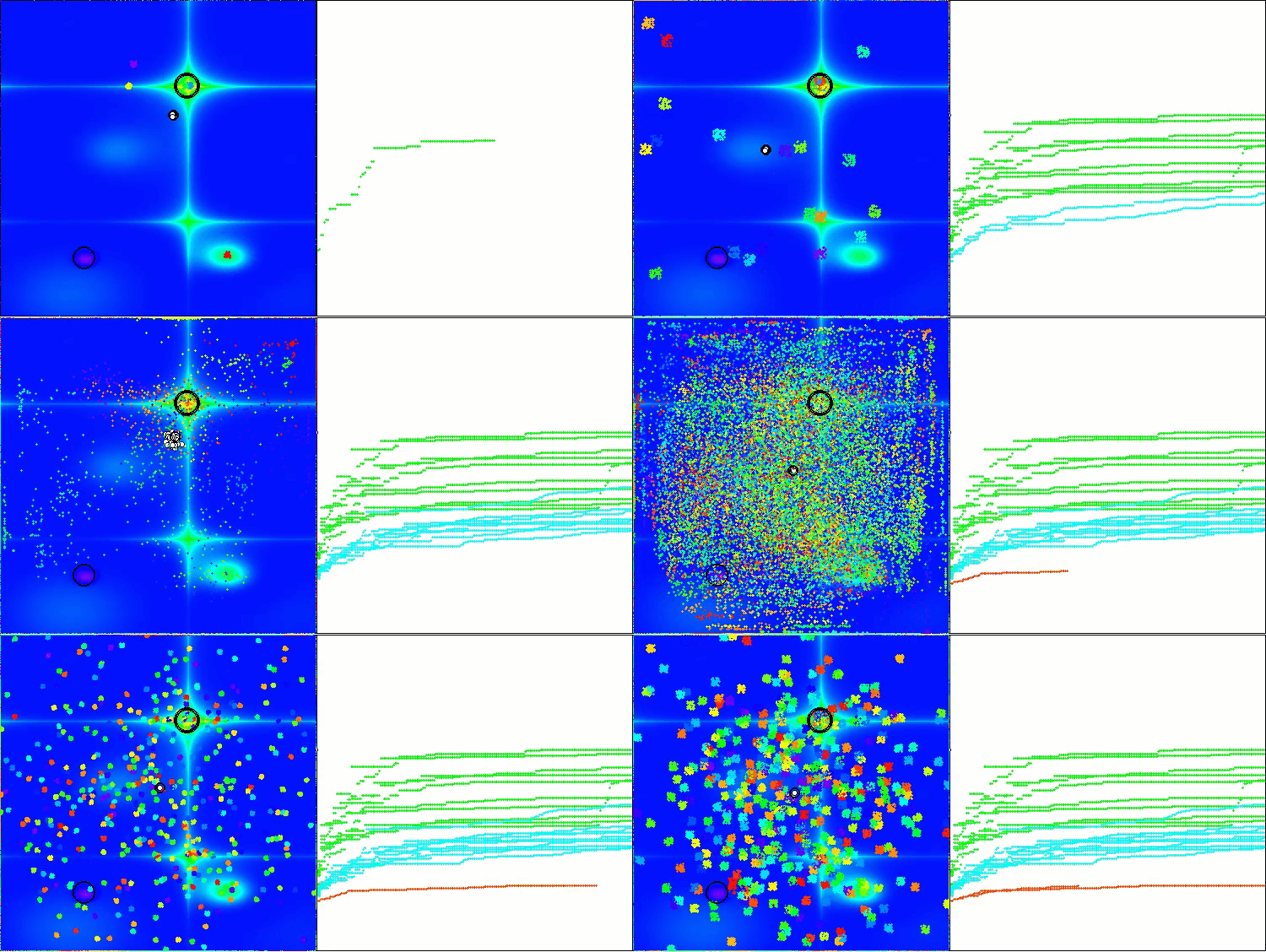
BHAm on the Forest test function

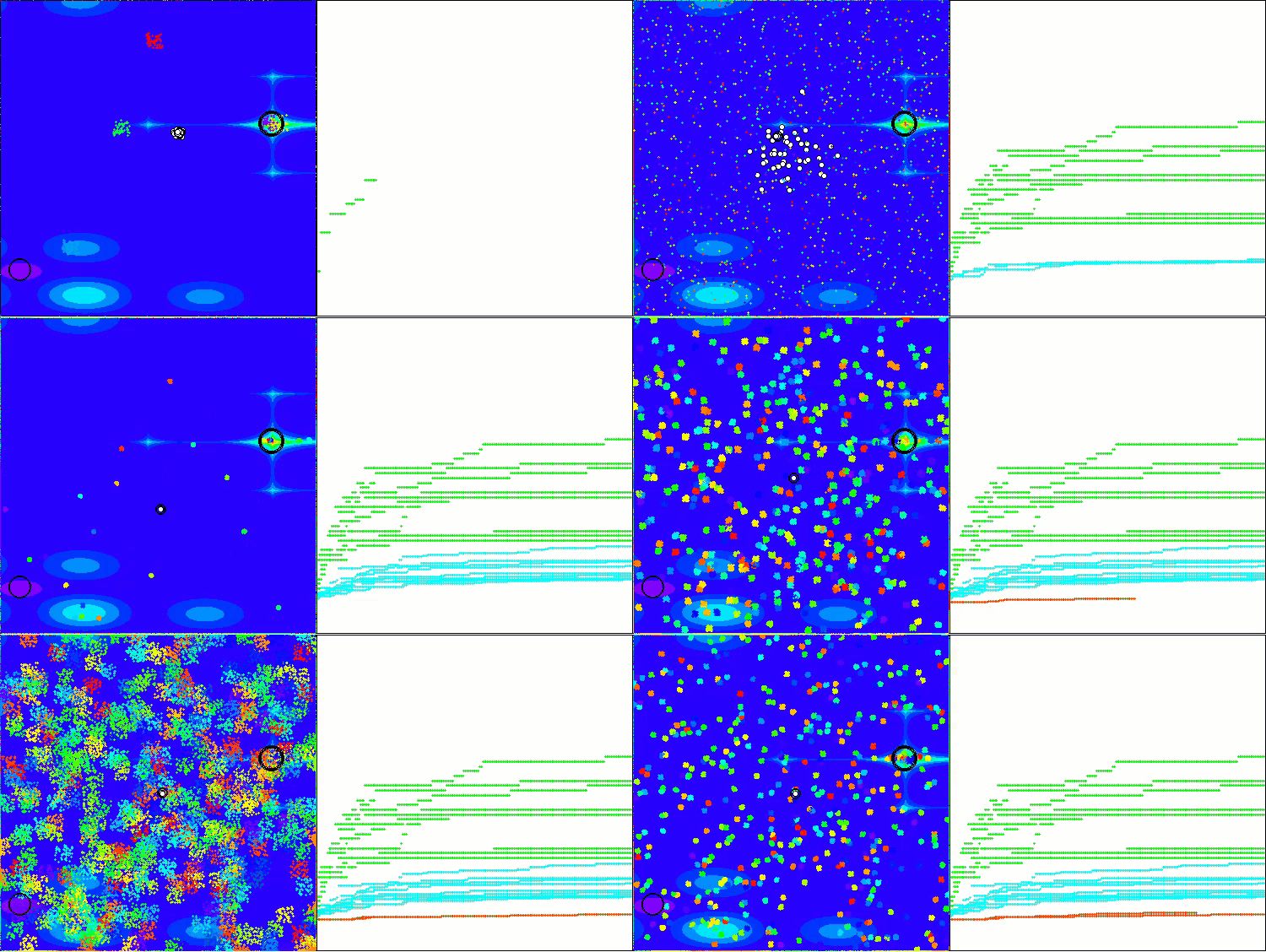
BHAm on the Megacity test function

The revised BBBC version finished 43rd in the rating table. RW is displayed as a standard of the lower limit of the "meaningfulness" of search strategies.

#	AO	Description	Hilly			Hilly final	Forest			Forest final	Megacity (discrete)			Megacity final	Final result	% of MAX
			10 p (5 F)	50 p (25 F)	1000 p (500 F)		10 p (5 F)	50 p (25 F)	1000 p (500 F)		10 p (5 F)	50 p (25 F)	1000 p (500 F)
1	ANS	across neighbourhood search	0.94948	0.84776	0.43857	2.23581	1.00000	0.92334	0.39988	2.32323	0.70923	0.63477	0.23091	1.57491	6.134	68.15
2	CLA	code lock algorithm (joo)	0.95345	0.87107	0.37590	2.20042	0.98942	0.91709	0.31642	2.22294	0.79692	0.69385	0.19303	1.68380	6.107	67.86
3	AMOm	animal migration ptimization M	0.90358	0.84317	0.46284	2.20959	0.99001	0.92436	0.46598	2.38034	0.56769	0.59132	0.23773	1.39675	5.987	66.52
4	(P+O)ES	(P+O) evolution strategies	0.92256	0.88101	0.40021	2.20379	0.97750	0.87490	0.31945	2.17185	0.67385	0.62985	0.18634	1.49003	5.866	65.17
5	CTA	comet tail algorithm (joo)	0.95346	0.86319	0.27770	2.09435	0.99794	0.85740	0.33949	2.19484	0.88769	0.56431	0.10512	1.55712	5.846	64.96
6	SDSm	stochastic diffusion search M	0.93066	0.85445	0.39476	2.17988	0.99983	0.89244	0.19619	2.08846	0.72333	0.61100	0.10670	1.44103	5.709	63.44
7	AAm	archery algorithm M	0.91744	0.70876	0.42160	2.04780	0.92527	0.75802	0.35328	2.03657	0.67385	0.55200	0.23738	1.46323	5.548	61.64
8	ESG	evolution of social groups (joo)	0.99906	0.79654	0.35056	2.14616	1.00000	0.82863	0.13102	1.95965	0.82333	0.55300	0.04725	1.42358	5.529	61.44
9	SIA	simulated isotropic annealing (joo)	0.95784	0.84264	0.41465	2.21513	0.98239	0.79586	0.20507	1.98332	0.68667	0.49300	0.09053	1.27020	5.469	60.76
10	ACS	artificial cooperative search	0.75547	0.74744	0.30407	1.80698	1.00000	0.88861	0.22413	2.11274	0.69077	0.48185	0.13322	1.30583	5.226	58.06
11	BHAm	black hole algorithm M	0.75236	0.76675	0.34583	1.86493	0.93593	0.80152	0.27177	2.00923	0.65077	0.51646	0.15472	1.32195	5.196	57.73
12	ASO	anarchy society optimization	0.84872	0.74646	0.31465	1.90983	0.96148	0.79150	0.23803	1.99101	0.57077	0.54062	0.16614	1.27752	5.178	57.54
13	AOSm	atomic orbital search M	0.80232	0.70449	0.31021	1.81702	0.85660	0.69451	0.21996	1.77107	0.74615	0.52862	0.14358	1.41835	5.006	55.63
14	TSEA	turtle shell evolution algorithm (joo)	0.96798	0.64480	0.29672	1.90949	0.99449	0.61981	0.22708	1.84139	0.69077	0.42646	0.13598	1.25322	5.004	55.60
15	DE	differential evolution	0.95044	0.61674	0.30308	1.87026	0.95317	0.78896	0.16652	1.90865	0.78667	0.36033	0.02953	1.17653	4.955	55.06
16	CRO	chemical reaction optimization	0.94629	0.66112	0.29853	1.90593	0.87906	0.58422	0.21146	1.67473	0.75846	0.42646	0.12686	1.31178	4.892	54.36
17	BSA	bird swarm algorithm	0.89306	0.64900	0.26250	1.80455	0.92420	0.71121	0.24939	1.88479	0.69385	0.32615	0.10012	1.12012	4.809	53.44
18	HS	harmony search	0.86509	0.68782	0.32527	1.87818	0.99999	0.68002	0.09590	1.77592	0.62000	0.42267	0.05458	1.09725	4.751	52.79
19	SSG	saplings sowing and growing	0.77839	0.64925	0.39543	1.82308	0.85973	0.62467	0.17429	1.65869	0.64667	0.44133	0.10598	1.19398	4.676	51.95
20	BCOm	bacterial chemotaxis optimization M	0.75953	0.62268	0.31483	1.69704	0.89378	0.61339	0.22542	1.73259	0.65385	0.42092	0.14435	1.21912	4.649	51.65
21	ABO	african buffalo optimization	0.83337	0.62247	0.29964	1.75548	0.92170	0.58618	0.19723	1.70511	0.61000	0.43154	0.13225	1.17378	4.634	51.49
22	(PO)ES	(PO) evolution strategies	0.79025	0.62647	0.42935	1.84606	0.87616	0.60943	0.19591	1.68151	0.59000	0.37933	0.11322	1.08255	4.610	51.22
23	TSm	tabu search M	0.87795	0.61431	0.29104	1.78330	0.92885	0.51844	0.19054	1.63783	0.61077	0.38215	0.12157	1.11449	4.536	50.40
24	BSO	brain storm optimization	0.93736	0.57616	0.29688	1.81041	0.93131	0.55866	0.23537	1.72534	0.55231	0.29077	0.11914	0.96222	4.498	49.98
25	WOAm	wale optimization algorithm M	0.84521	0.56298	0.26263	1.67081	0.93100	0.52278	0.16365	1.61743	0.66308	0.41138	0.11357	1.18803	4.476	49.74
26	AEFA	artificial electric field algorithm	0.87700	0.61753	0.25235	1.74688	0.92729	0.72698	0.18064	1.83490	0.66615	0.11631	0.09508	0.87754	4.459	49.55
27	AEO	artificial ecosystem-based optimization algorithm	0.91380	0.46713	0.26470	1.64563	0.90223	0.43705	0.21400	1.55327	0.66154	0.30800	0.28563	1.25517	4.454	49.49
28	ACOm	ant colony optimization M	0.88190	0.66127	0.30377	1.84693	0.85873	0.58680	0.15051	1.59604	0.59667	0.37333	0.02472	0.99472	4.438	49.31
29	BFO-GA	bacterial foraging optimization - ga	0.89150	0.55111	0.31529	1.75790	0.96982	0.39612	0.06305	1.42899	0.72667	0.27500	0.03525	1.03692	4.224	46.93
30	SOA	simple optimization algorithm	0.91520	0.46976	0.27089	1.65585	0.89675	0.37401	0.16984	1.44060	0.69538	0.28031	0.10852	1.08422	4.181	46.45
31	ABHA	artificial bee hive algorithm	0.84131	0.54227	0.26304	1.64663	0.87858	0.47779	0.17181	1.52818	0.50923	0.33877	0.10397	0.95197	4.127	45.85
32	ACMO	atmospheric cloud model optimization	0.90321	0.48546	0.30403	1.69270	0.80268	0.37857	0.19178	1.37303	0.62308	0.24400	0.10795	0.97503	4.041	44.90
33	ADAMm	adaptive moment estimation M	0.88635	0.44766	0.26613	1.60014	0.84497	0.38493	0.16889	1.39880	0.66154	0.27046	0.10594	1.03794	4.037	44.85
34	ATAm	artificial tribe algorithm M	0.71771	0.55304	0.25235	1.52310	0.82491	0.55904	0.20473	1.58867	0.44000	0.18615	0.09411	0.72026	3.832	42.58
35	ASHA	artificial showering algorithm	0.89686	0.40433	0.25617	1.55737	0.80360	0.35526	0.19160	1.35046	0.47692	0.18123	0.09774	0.75589	3.664	40.71
36	ASBO	adaptive social behavior optimization	0.76331	0.49253	0.32619	1.58202	0.79546	0.40035	0.26097	1.45677	0.26462	0.17169	0.18200	0.61831	3.657	40.63
37	MEC	mind evolutionary computation	0.69533	0.53376	0.32661	1.55569	0.72464	0.33036	0.07198	1.12698	0.52500	0.22000	0.04198	0.78698	3.470	38.55
38	IWO	invasive weed optimization	0.72679	0.52256	0.33123	1.58058	0.70756	0.33955	0.07484	1.12196	0.42333	0.23067	0.04617	0.70017	3.403	37.81
39	Micro-AIS	micro artificial immune system	0.79547	0.51922	0.30861	1.62330	0.72956	0.36879	0.09398	1.19233	0.37667	0.15867	0.02802	0.56335	3.379	37.54
40	COAm	cuckoo optimization algorithm M	0.75820	0.48652	0.31369	1.55841	0.74054	0.28051	0.05599	1.07704	0.50500	0.17467	0.03380	0.71347	3.349	37.21
41	SDOm	spiral dynamics optimization M	0.74601	0.44623	0.29687	1.48912	0.70204	0.34678	0.10944	1.15826	0.42833	0.16767	0.03663	0.63263	3.280	36.44
42	NMm	Nelder-Mead method M	0.73807	0.50598	0.31342	1.55747	0.63674	0.28302	0.08221	1.00197	0.44667	0.18667	0.04028	0.67362	3.233	35.92
43	BBBC	big bang-big crunch algorithm	0,60531	0,45250	0,31255	1,37036	0,52323	0,35426	0,20417	1,08166	0,39769	0,19431	0,11286	0,70486	3,157	35,08
44	FAm	firefly algorithm M	0.58634	0.47228	0.32276	1.38138	0.68467	0.37439	0.10908	1.16814	0.28667	0.16467	0.04722	0.49855	3.048	33.87
45	GSA	gravitational search algorithm	0.64757	0.49197	0.30062	1.44016	0.53962	0.36353	0.09945	1.00260	0.32667	0.12200	0.01917	0.46783	2.911	32.34
	RW	random walk	0.48754	0.32159	0.25781	1.06694	0.37554	0.21944	0.15877	0.75375	0.27969	0.14917	0.09847	0.52734	2.348	26.09

Summary

The BBBC (Big Bang-Big Crunch) algorithm is an interesting approach to global optimization inspired by cosmological processes. However, test results show that its claimed efficiency is exaggerated. It is important to note that the algorithm concentrates the search in the center of the space, which can create the illusion of high search capabilities. This does not indicate the outstanding capabilities of the algorithm, but rather the coincidence of the problem conditions with its features.

It is also worth mentioning that many standard test functions used to evaluate algorithms have a global optimum located in the center of the search space. Such tests are not always reliable and can be misleading about the actual search capabilities of algorithms such as BBBC, which have "hacking" features in their search strategy. Therefore, sometimes widely known "truths" should be treated with caution and critical thinking.

However, the modified version of the BBBC algorithm demonstrates good results on high-dimensional problems, which highlights its potential for development. This opens up new opportunities for further research and improvements that can improve its performance in more complex and diverse optimization problems, as well as enrich our knowledge base with new techniques for finding optimal solutions.

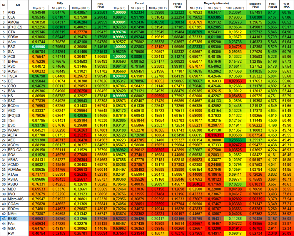
Figure 2. Color gradation of algorithms according to relevant tests Results greater than or equal to 0.99 are highlighted in white

The color gradation in the table clearly illustrates that not all optimization algorithms are more efficient than simple random search (RW), especially for some types of problems. This is especially evident in the context of multidimensional problems, where the complexity of the terrain and the dimensionality of the search space increase significantly. In such cases, many traditional strategies may lose their efficiency, facing problems associated with local extremes, the curse of dimensionality, and other factors. However, this does not mean that we advocate using random search as a primary method, but it is important to compare it to better understand the limitations and capabilities of different optimization strategies.

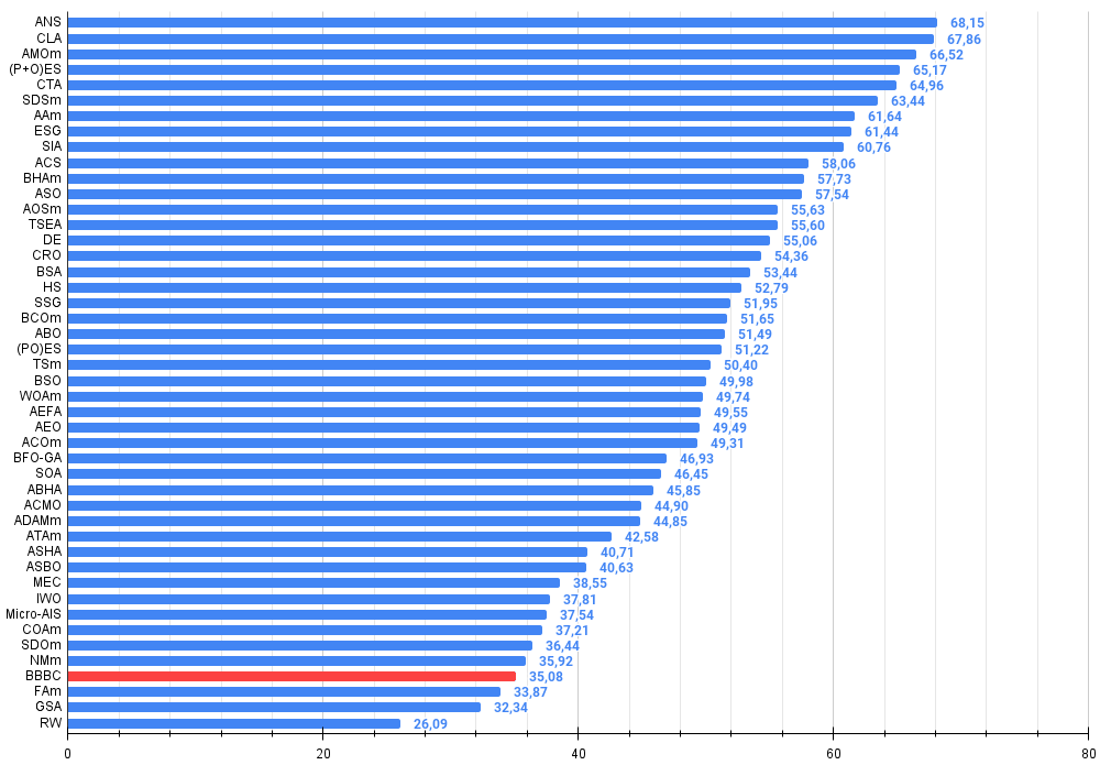
Figure 3. Histogram of algorithm testing results (scale from 0 to 100, the higher the better, where 100 is the maximum possible theoretical result, in the archive there is a script for calculating the rating table)

BBBC pros and cons:

Pros:

1. The only external parameter is the population size.
   
2. Simple implementation.
3. Very fast EA.
4. Works well on large-scale problems.
   

Disadvantages:

1. Large scatter of results on small-dimensional problems.
   
2. Tendency to get stuck on low-dimensional problems.
   

The article is accompanied by an archive with the current versions of the algorithm codes. The author of the article is not responsible for the absolute accuracy in the description of canonical algorithms. Changes have been made to many of them to improve search capabilities. The conclusions and judgments presented in the articles are based on the results of the experiments.

• github: https://github.com/JQSakaJoo/Population-optimization-algorithms-MQL5

Programs used in the article

#	Name	Type	Description
1	#C_AO.mqh	Include	Parent class of population optimization algorithms
2	#C_AO_enum.mqh	Include	Enumeration of population optimization algorithms
3	TestFunctions.mqh	Include	Library of test functions
4	TestStandFunctions.mqh	Include	Test stand function library
5	Utilities.mqh	Include	Library of auxiliary functions
6	CalculationTestResults.mqh	Include	Script for calculating results in the comparison table
7	Testing AOs.mq5	Script	The unified test stand for all population optimization algorithms
8	Simple use of population optimization algorithms.mq5	Script	A simple example of using population optimization algorithms without visualization
9	Test_AO_BBBC.mq5	Script	BBBC test stand