Population optimization algorithms: Stochastic Diffusion Search (SDS)

Contents

1. Introduction
2. Algorithm
3. Test results

1. Introduction

The Stochastic Diffusion Search (SDS) algorithm was proposed in 1989 by J. Bishop and was actively developed by Bishop and S. Nasuto. A distinctive feature of this algorithm is its deep mathematical justification in comparison with other population algorithms. SDS was originally developed for discrete optimization. In 2011, its modification for global continuous optimization was proposed.

Interesting facts:

1. Stochastic Diffusion Search (SDS) was the first Swarm Intelligence metaheuristic, which belongs to the family of swarm intelligence and natural search and optimization algorithms. Other examples of such algorithms are ant colony optimization, particle swarm optimization and genetic algorithms.

2. Unlike ant colony optimization based on stigmergy communication, SDS uses direct communication between agents, similar to the tandem calling mechanism used by Leptothorax acervorum ants.

The SDS algorithm is based on low-cost partial evaluation of a hypothesis (a candidate solution to a search problem) by agents. The agents then exchange information about the hypotheses through direct personal communication. Through the diffusion mechanism, high-quality solutions can be identified from clusters of agents with the same hypothesis.

To better understand the operation of the SDS algorithm, we can use a simple analogy - the Restaurant Game.

In the restaurant game, participants play the role of agents, and restaurants play the role of hypotheses. Each agent selects a restaurant to eat at based on their preferences and information they receive from other agents. The agents then exchange information about their choices and preferences. As a result of this process, clusters of agents who have chosen the same restaurant are formed and can be identified as potentially good decisions.

The SDS algorithm has several advantages. First, it allows agents to make cheap partial hypothesis estimates, which reduces the computational complexity of the algorithm. Secondly, it uses direct personal communication between agents, which allows information to be disseminated efficiently. Third, SDS is mathematically based, making it more reliable and predictable.

However, the SDS algorithm also has its limitations. First, it can only be effective in certain types of problems where the concept of a hypothesis is applicable. Second, it may suffer from the problem of premature convergence, where agents converge on one hypothesis too quickly without exploring other possibilities. Third, the algorithm requires parameter tuning, which can be a complex and time-consuming process. The restrictions have been voiced by some authors. Let's check if they are justified.

Overall, SDS is an interesting and efficient algorithm for solving optimization problems. It combines the advantages of population algorithms and mathematical rationale, making it attractive for research and application in various fields.

2. Algorithm

Let's move on to a more detailed consideration of the SDS algorithm.

Stochastic Diffusion Search (SDS) is a population algorithm based on two search strategy ideas:

1. Partial evaluation of solutions.
2. Dissemination of promising solutions throughout the population.

There are two canonical games that describe in simple terms how SDS works.
1. Restaurant game
2. Gold mining game.

Restaurant game

A group of delegates is at a long conference in an unfamiliar city. Every evening they are faced with the problem of choosing a restaurant for dinner. The city has a huge number of restaurants offering a variety of dishes. The group's goal is to find the best one where each delegate can enjoy a meal. However, conducting an exhaustive search of all possible combinations of restaurants and dishes would take too much time. To solve this problem, delegates resort to using stochastic diffusion search.

Each delegate acts as an agent who makes a guess regarding the selection of the best restaurant in the city. Each evening, delegates test their hypotheses by visiting restaurants and randomly choosing one offer from the restaurant's selection of dishes. The next morning, at breakfast, each delegate who was dissatisfied with the dinner the previous evening asks one of his or her colleagues to share their impressions of the dinner. If the colleague's impressions are positive, the delegate also chooses that restaurant. Otherwise, the delegate randomly selects another place from the list of available restaurants in that city.

Thus, thanks to this strategy, a significant number of delegates are quickly formed, gathering around the best restaurant in the city.

The game has several interesting features. In the complete absence of external control and management, a group of delegates communicate to solve a problem that cannot be solved quickly alone. If the current restaurant's service or menu significantly declines or the business closes, delegates effectively move on to the next best restaurant. The main requirement is the comparability of restaurants, menus and individual dishes. Each agent decides for themselves whether their experience was good.

Delegates spend many evenings in a high-quality restaurant before all the dishes in all the locations in the city are assessed.
Critics point out that delegates are likely to have different food preferences, so one delegate may find a restaurant where they like all the dishes, but it may not satisfy the rest of the group. If only one or a small number of delegates remain permanently in such a restaurant, the rest continue to act as usual, and in the end the majority still gathers at the best restaurant. However, in extreme cases, all agents may find themselves dining alone, even if there is a single excellent restaurant that will satisfy the majority of the delegates. This restaurant will never be found, as all delegates are satisfied with their current selections and will not look for new places.

Our implementation makes small changes to the logic of the search strategy, thanks to which delegates continue searching for restaurants even when there is no delegate with better experience, thus the search for restaurants does not stop, unlike the canonical version, in which the fact of changing the current opinion is important about a restaurant from the previous one. If the opinion does not change for the better among the majority of delegates, then they will continue to go to the same restaurant, which means getting stuck in a local extreme.

Gold mining game

A group of friends, consisting of experienced miners, learn about the possibility of mining gold in the hills of a mountain range. However, they have no information about where exactly the richest place is located. On their maps, the mountain range is divided into several individual hills, each containing a set of strata that require mining. The probability of discovering gold over time is proportional to its wealth.

To maximize their collective wealth, miners should identify the hill with the richest seams of gold so that the maximum number of miners can mine there. However, this information is not available in advance. To solve this problem, miners decide to use simple stochastic diffusion search.

The mining process begins with each miner being randomly assigned a hill to mine (custom hill hypothesis). Every day, each miner randomly selects a seam on their hill to mine.

At the end of each day, the probability that the miner is happy is proportional to the amount of gold he or she found (the value of the fitness function).
In the evening, after finishing work, the miners get together. An unhappy miner randomly selects another miner to talk to. If the chosen miner is satisfied, he gladly tells his colleague the name of the hill he is mining. Thus, both miners support the hill hypothesis. If the chosen miner is unhappy, he says nothing, and the original miner is again forced to choose a new hypothesis - identifying the hill he will mine the next day at random.

In the context of SDS (self-organizing dynamic systems), agents act as miners. Active agents are "happy miners" and inactive agents are "unhappy miners". Each agent's hypothesis represents the miner's "hill hypothesis". This process is isomorphic to SDS allowing miners to naturally self-organize and quickly converge on the hill(s) of a mountain ridge with a high concentration of gold.

Miners' happiness can be measured probabilistically or represented as an absolute Boolean value, given that every miner is either happy or unhappy at the end of each day. If gold is modeled as a limited resource that decreases over time, then the search becomes quite adaptive, and miners move to places with the most gold.

Although the term "happy" is subjective, like eating habits, in this case it is used in an objective sense. All miners use the same process: the amount of gold they find in a day determines the likelihood that they will declare themselves "lucky" at the end of the day, when they get together to potentially share information about the hills they are mining.

We will not use the division of miners into "happy" and "unhappy" ones. As in the case of the restaurant game concept, this allows increasing the activity of agents in searching for new unexplored places.

To formalize the algorithm, we will use the concept of "candidate", which is equivalent to a delegate in the restaurant game and a miner in the gold mining game. The candidate is a search agent. For a simpler understanding of the essence of a restaurant or a hill, we can imagine a space with two coordinates, although in reality an unlimited number of coordinates can be used to solve multidimensional problems. In Figure 1, the designations C1, C2, C3 show candidates that store restaurant numbers (the corresponding spaces in the search field). In the process of diffusion exchange of information about restaurants, candidates borrow restaurant numbers from randomly selected conference participants if the fitness function value of the interlocutor is higher. The range of each optimization parameter (search space coordinates) is divided by the number of restaurants specified in the external parameters of the algorithm. For example, if the number of 100 restaurants is specified in the algorithm parameters, this means the range of each coordinate will be divided into 100 parts.

Each restaurant offers a list of dishes on the menu. Each menu dish is a specific coordinate of the search space within one restaurant. The algorithm implements a scheme, in which the candidate tastes only one randomly selected restaurant dish.

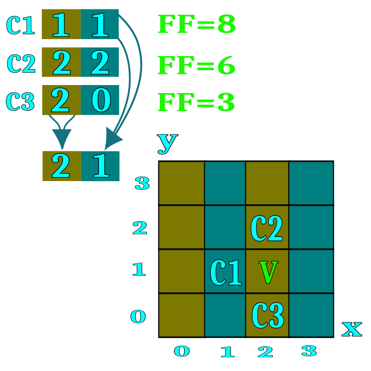
Figure 1. A visual representation of the diffusion principle of restaurant information exchange

Let's look at the steps of the SDS algorithm in the form of a pseudocode.

1. Initialization of candidates (assigning random restaurants and dishes).

2.0. Hypothesis testing and diffusion exchange between candidates.

2.1. Compare the candidate's current experience with his or her previous experience.

2.1.1. If the experience is better, assign restaurant addresses as a hypothesis for the next iteration.

2.1.2. If the experience is worse, then ask the opinion of a randomly selected candidate.

2.1.2.1. If the experience of the interlocutor (the candidate) is better, then take the addresses of promising (for the current candidate) restaurants.

2.1.2.2. If the experience of the interlocutor - the candidate - is worse, then with a degree of probability we either choose the address of a randomly selected restaurant or keep the current one.

3.0. Select dishes from the generated list of restaurants as a hypothesis for the next iteration.

The logical diagram of hypothesis testing is presented in Figure 2. Most of the logic circuit performs the task of selecting a restaurant, and after the restaurant selection is completed, a dish is randomly selected. The choice of a restaurant is the main task of the algorithm, but the choice of a dish is completely random and independent of previous iterations.

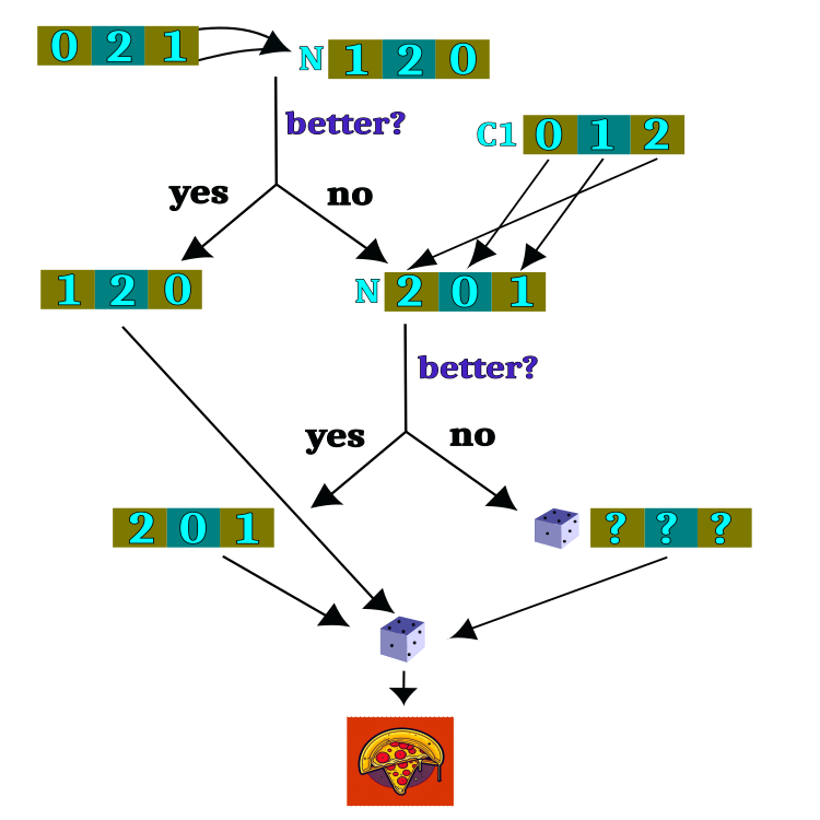
Figure 2. Logical scheme for testing hypotheses

It is time to look at the SDS (Stochastic Diffusion Search) code and start with the heart and soul of the algorithm - the agent, aka the candidate, which can be described by the S_Candidate structure. It contains the following fields:

1. raddr: array containing restaurant addresses. Each array element represents the address of one restaurant.
2. raddrPrev: array containing previous restaurant addresses. Each array element represents the address of one restaurant.
3. c: array containing the coordinates (dishes). Each element of the array represents the coordinate of one dish.
4. cPrev: array containing the previous coordinates (dishes). Each element of the array represents the coordinate of one dish.
5. f: fitness function value for the current state of the agent.
6. fPrev: fitness function value for the previous state of the agent.

The S_Candidate structure has the Init method, which initializes all arrays of 'coords' size (the number of coordinates - parameters to be optimized) and sets the initial values of f and fPrev to -DBL_MAX, since there is nothing and no one to compare the candidate’s experience with at the first iteration.

//——————————————————————————————————————————————————————————————————————————————
struct S_Candidate
{
  void Init (int coords)
  {
    ArrayResize (c,         coords);
    ArrayResize (cPrev,     coords);
    ArrayResize (raddr,     coords);
    ArrayResize (raddrPrev, coords);
    f        = -DBL_MAX;
    fPrev    = -DBL_MAX;
  }
  int    raddr     []; //restaurant address
  int    raddrPrev []; //previous restaurant address
  double c         []; //coordinates (dishes)
  double cPrev     []; //previous coordinates (dishes)
  double f;            //fitness
  double fPrev;        //previous fitness
};
//——————————————————————————————————————————————————————————————————————————————

Declare an SDS algorithm class containing the following:

Class fields:
- cB: array containing the best coordinates
- fB: fitness function value for the best coordinates
- cands: array of candidates for finding optimal coordinates
- rangeMax: array containing the maximum values for each coordinate
- rangeMin: array containing the minimum values for each coordinate
- rangeStep: array containing search steps for each coordinate

Class methods:
- Init: initialization of algorithm parameters such as number of coordinates, population size, number of restaurants and probability of choosing a restaurant
- Moving: performing an algorithm step, moving candidates to new coordinates
- Revision: performing revision step, updating best coordinates and fitness functions
- SeInDiSp: method for calculating a new coordinate in a given range with a given step
- RNDfromCI: method for generating a random number in a given interval

Other class fields:
- coords: number of coordinates
- populationSize: population size
- restNumb: number of restaurants
- probabRest: probability of choosing a restaurant
- restSpace: restaurant space
- revision: flag indicating the need for a revision

//——————————————————————————————————————————————————————————————————————————————
class C_AO_SDS
{
  //----------------------------------------------------------------------------
  public: double cB   [];       //best coordinates
  public: double fB;            //FF of the best coordinates
  public: S_Candidate cands []; //candidates

  public: double rangeMax  []; //maximum search range
  public: double rangeMin  []; //manimum search range
  public: double rangeStep []; //step search



  public: void Init (const int    coordinatesNumberP,   //coordinates number
                     const int    populationSizeP,      //population size
                     const int    restaurantsNumberP,   //restaurants number
                     const double probabRestP);         //probability restaurant choosing

  public: void Moving   ();
  public: void Revision ();

  //----------------------------------------------------------------------------
  private: int    coords;            //coordinates number
  private: int    populationSize;    //population size

  private: int    restNumb;          //restaurants number
  private: double probabRest;        //probability restaurant choosing
  private: double restSpace [];      //restaurants space

  private: bool   revision;

  private: double SeInDiSp  (double In, double InMin, double InMax, double Step);
  private: double RNDfromCI (double min, double max);
};
//——————————————————————————————————————————————————————————————————————————————

The initialization method of the SDS algorithm begins by setting initial values for some variables and arrays.

The input parameters of the method are:
- coordinatesNumberP: number of coordinates (search space dimension)
- populationSizeP: population size (number of candidates)
- restaurantsNumberP: number of restaurants
- probabRestP: probability of choosing a restaurant

First, the random number generator is reset using the MathSrand function and passing it the current value of microseconds. The fB and revision variables are then initialized to the initial values -DBL_MAX and 'false', respectively.
Next, the values of the coordinatesNumberP and populationSizeP inputs are assigned to coords and populationSize variables.
The restNumb and probabRest variables are initialized with the restaurantsNumberP and probabRestP values.
The restSpace array of 'coords' size is created using the ArrayResize function.
The 'cands' array of populationSize size is then created using the ArrayResize function. In the loop, each element of the 'cands' array is initialized by calling the Init method with the 'coords' parameter.
The rangeMax, rangeMin, rangeStep and cB arrays of the 'coords' size are also created using the ArrayResize function.

//——————————————————————————————————————————————————————————————————————————————
void C_AO_SDS::Init (const int    coordinatesNumberP,   //coordinates number
                     const int    populationSizeP,      //population size
                     const int    restaurantsNumberP,   //restaurants number
                     const double probabRestP)          //probability restaurant choosing
{
  MathSrand ((int)GetMicrosecondCount ()); // reset of the generator
  fB       = -DBL_MAX;
  revision = false;

  coords         = coordinatesNumberP;
  populationSize = populationSizeP;

  restNumb   = restaurantsNumberP;
  probabRest = probabRestP;
  ArrayResize (restSpace, coords);

  ArrayResize (cands, populationSize);
  for (int i = 0; i < populationSize; i++) cands [i].Init (coords);

  ArrayResize (rangeMax,       coords);
  ArrayResize (rangeMin,       coords);
  ArrayResize (rangeStep,      coords);
  ArrayResize (cB,             coords);
}
//——————————————————————————————————————————————————————————————————————————————

Although the Moving() method will be called at each iteration, the main logic of the method is executed only once controlled by the revision flag.

At the beginning of the function, the 'revision' variable is checked. If it is 'false', then the variables and arrays are initialized.
Then a loop occurs along the coordinates of points in space.

Inside this loop, restSpace[i] is calculated, which is the length of the interval for each coordinate, defined as the difference between the maximum and minimum values of the range divided by restNumb.

Next, the variables min and max are declared, which will be used to determine the range of values for the space of a particular restaurant.

The n and dish variables are then initialized to be used to determine random values within the range of the selected restaurant.

Then a loop is executed through the population of populationSize size, within which a loop is executed over the coordinates of the space points. Inside this loop, a random number n is generated using the RNDfromCI() function, which is used to determine the index in the restSpace array. If the resulting value n is greater than or equal to restNumb, then it is assigned restNumb - 1, to ensure a uniform distribution of the random variable. The min and max values are then calculated using rangeMin, restSpace and n.

We generate a random number 'dish' using the RNDfromCI() function, which is in the range from 'min' to 'max' (restaurant space).

The value of 'dish' is then used to calculate the value of c[i] using the SeInDiSp() function, which uses rangeMin, rangeMax and rangeStep to ensure the correct step of the optimized parameters.

As a result of this algorithm, each point in space receives random values for each coordinate in accordance with the space of the restaurant, simulating a random choice of dish.

The 'revision' variable is set to 'true' so that the next time the Moving() function is called, the variables and arrays are not initialized.

//——————————————————————————————————————————————————————————————————————————————
void C_AO_SDS::Moving ()
{
  if (!revision)
  {
    for (int i = 0; i < coords; i++)
    {
      restSpace [i] = (rangeMax [i] - rangeMin [i]) / restNumb;
    }

    double min = 0.0;
    double max = 0.0;

    int    n   = 0;
    double dish = 0.0;

    for (int i = 0; i < populationSize; i++)
    {
      for (int c = 0; c < coords; c++)
      {
        n = (int)(RNDfromCI (0, restNumb));
        if (n >= restNumb) n = restNumb - 1;

        cands [i].raddr     [c] = n;
        cands [i].raddrPrev [c] = n;
        min = rangeMin [c] + restSpace [c] * n;
        max = min + restSpace [c];

        dish = RNDfromCI (min, max);

        cands [i].c [c] =  SeInDiSp (dish, rangeMin [c], rangeMax [c], rangeStep [c]);
      }
    }

    revision = true;
  }
}
//——————————————————————————————————————————————————————————————————————————————

The Revision method of the SDS algorithm performs the basic logic for selecting restaurants and restaurant dishes. This is not typical for the algorithms discussed earlier, in which the main logic for moving agents was located in the Moving method, although the order of calling the algorithm methods remains the same and corresponds to the concept chosen in the first article of the series. The algorithm consists of the following steps:

1. Updating the best found value of the fB fitness function and the corresponding cB set of coordinates. For each candidate i in the population, a comparison is made, if the value of f (the function estimate) is greater than the current global value of fB, then fB is updated and copied from i candidate to the cB best global coordinate set.

2. Updating previous ratings and restaurant sets for each candidate. For each i candidate in the population, if the value of f is greater than the previous value of fPrev, then fPrev is updated, and the sets of restaurants c and raddr from i candidate are copied to the corresponding previous values of cPrev and raddrPrev.

3. Selecting a new set of restaurants for each candidate. For each i candidate in the population and each c coordinate, a random number n is selected ranging from 0 to populationSize. If the value of fPrev for candidate n is greater than the value of fPrev for candidate i, then the set of restaurants raddr for candidate i is updated with the raddrPrev value for n candidate. Otherwise, a random number rnd is generated in the range from 0.0 to 1.0. If rnd is less than the probabRest probability, then the n random number in the range from 0 to restNumb is selected and the set of restaurants raddr for i candidate is updated with the value of n. Otherwise, the raddr set of restaurants for i candidate remains unchanged.

4. Generating a new set of coordinates for each candidate. The 'min' and 'max' minimum and maximum values are determined for each i candidate in the population and each c coordinate, based on the rangeMin and restSpace for the corresponding coordinate. A random number in the 'min' to 'max' range is then generated using the SeInDiSp function, and the resulting value is assigned to the corresponding c coordinate in the c set for i candidate.

Thus, the Revision method of the SDS algorithm iterates through the population of candidates, updates the best value found and the set of restaurants, selects new sets of restaurants and generates new sets of coordinates for each candidate.

//——————————————————————————————————————————————————————————————————————————————
void C_AO_SDS::Revision ()
{
  //----------------------------------------------------------------------------
  for (int i = 0; i < populationSize; i++)
  {
    if (cands [i].f > fB)
    {
      fB = cands [i].f;
      ArrayCopy (cB, cands [i].c, 0, 0, WHOLE_ARRAY);
    }
  }

  //----------------------------------------------------------------------------
  double min = 0.0;
  double max = 0.0;
  double rnd = 0.0;
  int    n   = 0;

  for (int i = 0; i < populationSize; i++)
  {
    if (cands [i].f > cands [i].fPrev)
    {
      cands [i].fPrev = cands [i].f;
      ArrayCopy (cands [i].cPrev, cands [i].c, 0, 0, WHOLE_ARRAY);
      ArrayCopy (cands [i].raddrPrev, cands [i].raddr, 0, 0, WHOLE_ARRAY);
    }
  }

  for (int i = 0; i < populationSize; i++)
  {
    for (int c = 0; c < coords; c++)
    {
      n = (int)(RNDfromCI (0, populationSize));
      if (n >= populationSize) n = populationSize - 1;

      if (cands [n].fPrev > cands [i].fPrev)
      {
        cands [i].raddr [c] = cands [n].raddrPrev [c];
      }
      else
      {
        rnd = RNDfromCI (0.0, 1.0);

        if (rnd < probabRest)
        {
          n = (int)(RNDfromCI (0, restNumb));
          if (n >= restNumb) n = restNumb - 1;
          cands [i].raddr [c] = n;
        }
        else
        {
          cands [i].raddr [c] = cands [i].raddrPrev [c];
        }
      }

      min = rangeMin [c] + restSpace [c] * cands [i].raddr [c];
      max = min + restSpace [c];

      cands [i].c [c] = SeInDiSp (RNDfromCI (min, max), rangeMin [c], rangeMax [c], rangeStep [c]);
    }
  }
}
//——————————————————————————————————————————————————————————————————————————————

3. Test results

Printout of the stochastic diffusion search algorithm operation on the test bench:

C_AO_SDS:100;1000;0.1
=============================
5 Rastrigin's; Func runs 10000 result: 80.64253803557851
Score: 0.99921
25 Rastrigin's; Func runs 10000 result: 79.00996143538204
Score: 0.97898
500 Rastrigin's; Func runs 10000 result: 54.31544686388126
Score: 0.67300
=============================
5 Forest's; Func runs 10000 result: 1.677891584229713
Score: 0.94910
25 Forest's; Func runs 10000 result: 1.4089003503272384
Score: 0.79694
500 Forest's; Func runs 10000 result: 0.2437939668372883
Score: 0.13790
=============================
5 Megacity's; Func runs 10000 result: 8.6
Score: 0.71667
25 Megacity's; Func runs 10000 result: 6.448
Score: 0.53733
500 Megacity's; Func runs 10000 result: 0.9551999999999999
Score: 0.07960
=============================
All score: 5.86873

Immediately looking at the print of the algorithm results, we can pay attention to the incredibly high results compared to other algorithms. A detailed comparison is presented in the table below.

Note the atypical behavior of the algorithm when visualizing the movement of agents. Agents are distributed in number evenly and proportionally to the height of the fitness function hill, demonstrating high quality of clustering at local extrema. It seems that not a single hill will be missed by the algorithm. We can also see the almost stepless increase in the convergence of the algorithm at each iteration, which indicates a low tendency to get stuck in local extrema. Even on the most complex Forest function with a sharp global extremum, no stepwise convergence is observed.

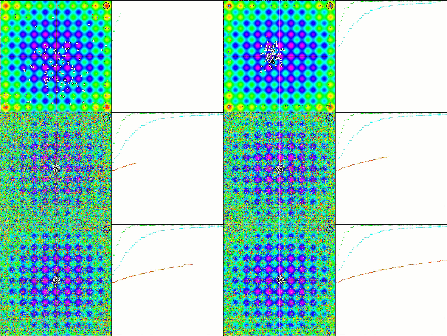
  SDS on the Rastrigin test function

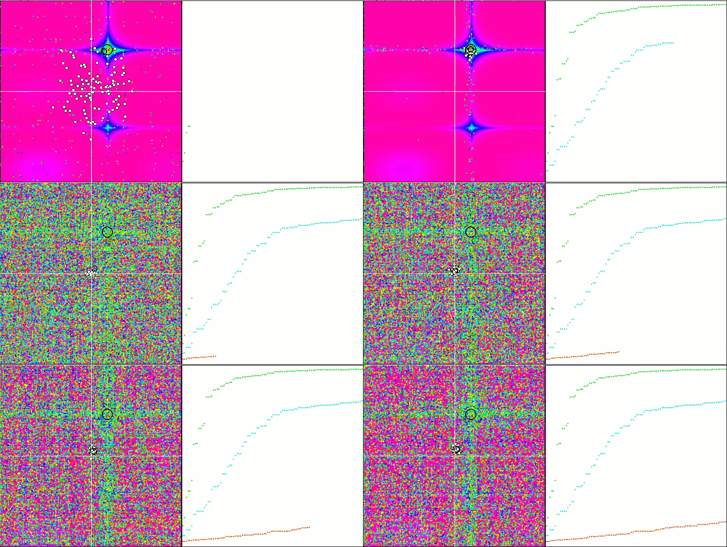
  SDS on the Forest test function

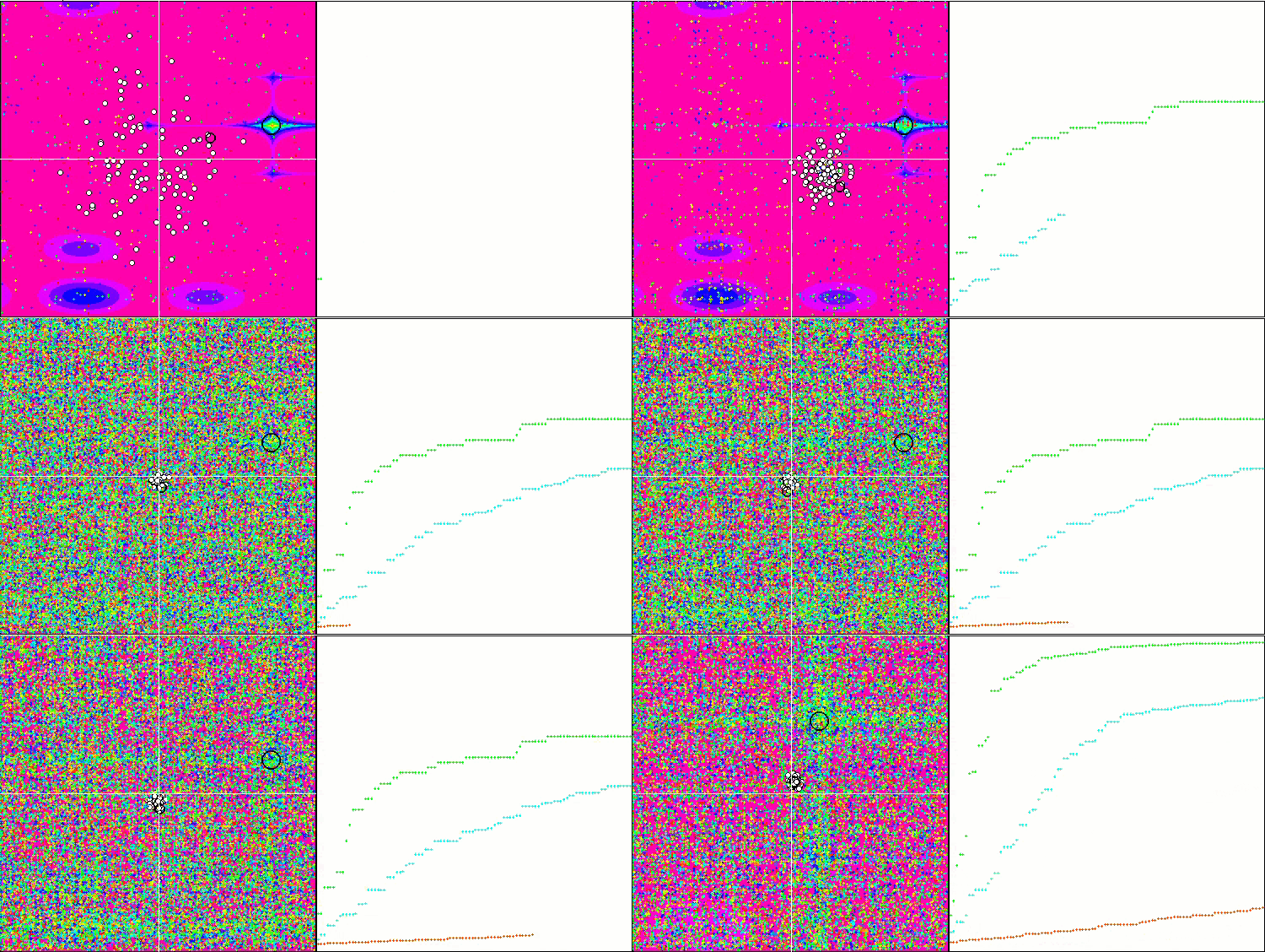
  SDS on the Megacity test function

I did not expect amazing results from such a very simple algorithm based on pure random walk. The SDS considerably outperformed (by almost 13%) all previously considered algorithms, demonstrating the best results in many tests (4 first places out of 9 possible ones). The only discipline is the multivariable Rastrigin function, in which the leader (the EM algorithm) has left everyone far behind.

Even on the extremely complex Megacity discrete function, the SDS algorithm performs excellently almost without being stuck anywhere. The only one to beat SDS in tests with 1000 variables on Forest and Megacity is the Growing Trees (SSG) algorithm. 

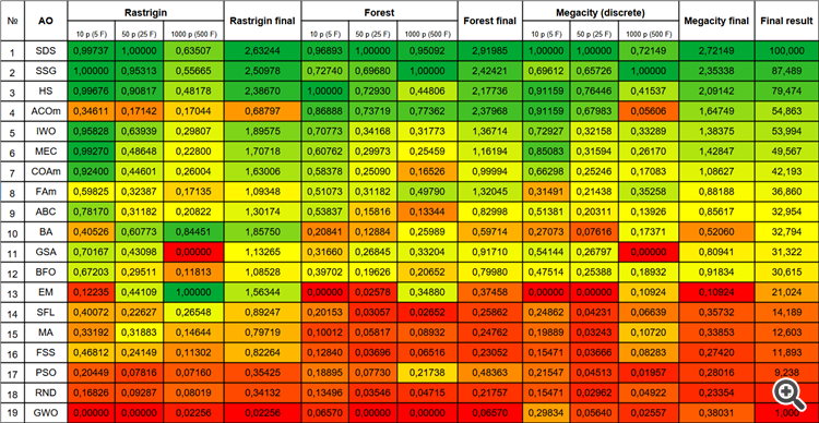
#	AO	Description	Rastrigin			Rastrigin final	Forest			Forest final	Megacity (discrete)			Megacity final	Final result
			10 p (5 F)	50 p (25 F)	1000 p (500 F)		10 p (5 F)	50 p (25 F)	1000 p (500 F)		10 p (5 F)	50 p (25 F)	1000 p (500 F)
1	SDS	stochastic diffusion search	0.99737	1.00000	0.63507	2.63244	0.96893	1.00000	0.95092	2.91985	1.00000	1.00000	0.72149	2.72149	100.000
2	SSG	saplings sowing and growing	1.00000	0.95313	0.55665	2.50978	0.72740	0.69680	1.00000	2.42421	0.69612	0.65726	1.00000	2.35338	87.489
3	HS	harmony search	0.99676	0.90817	0.48178	2.38670	1.00000	0.72930	0.44806	2.17736	0.91159	0.76446	0.41537	2.09142	79.474
4	ACOm	ant colony optimization M	0.34611	0.17142	0.17044	0.68797	0.86888	0.73719	0.77362	2.37968	0.91159	0.67983	0.05606	1.64749	54.863
5	IWO	invasive weed optimization	0.95828	0.63939	0.29807	1.89575	0.70773	0.34168	0.31773	1.36714	0.72927	0.32158	0.33289	1.38375	53.994
6	MEC	mind evolutionary computation	0.99270	0.48648	0.22800	1.70718	0.60762	0.29973	0.25459	1.16194	0.85083	0.31594	0.26170	1.42847	49.567
7	COAm	cuckoo optimization algorithm M	0.92400	0.44601	0.26004	1.63006	0.58378	0.25090	0.16526	0.99994	0.66298	0.25246	0.17083	1.08627	42.193
8	FAm	firefly algorithm M	0.59825	0.32387	0.17135	1.09348	0.51073	0.31182	0.49790	1.32045	0.31491	0.21438	0.35258	0.88188	36.860
9	ABC	artificial bee colony	0.78170	0.31182	0.20822	1.30174	0.53837	0.15816	0.13344	0.82998	0.51381	0.20311	0.13926	0.85617	32.954
10	BA	bat algorithm	0.40526	0.60773	0.84451	1.85750	0.20841	0.12884	0.25989	0.59714	0.27073	0.07616	0.17371	0.52060	32.794
11	GSA	gravitational search algorithm	0.70167	0.43098	0.00000	1.13265	0.31660	0.26845	0.33204	0.91710	0.54144	0.26797	0.00000	0.80941	31.322
12	BFO	bacterial foraging optimization	0.67203	0.29511	0.11813	1.08528	0.39702	0.19626	0.20652	0.79980	0.47514	0.25388	0.18932	0.91834	30.615
13	EM	electroMagnetism-like algorithm	0.12235	0.44109	1.00000	1.56344	0.00000	0.02578	0.34880	0.37458	0.00000	0.00000	0.10924	0.10924	21.024
14	SFL	shuffled frog-leaping	0.40072	0.22627	0.26548	0.89247	0.20153	0.03057	0.02652	0.25862	0.24862	0.04231	0.06639	0.35732	14.189
15	MA	monkey algorithm	0.33192	0.31883	0.14644	0.79719	0.10012	0.05817	0.08932	0.24762	0.19889	0.03243	0.10720	0.33853	12.603
16	FSS	fish school search	0.46812	0.24149	0.11302	0.82264	0.12840	0.03696	0.06516	0.23052	0.15471	0.03666	0.08283	0.27420	11.893
17	PSO	particle swarm optimisation	0.20449	0.07816	0.07160	0.35425	0.18895	0.07730	0.21738	0.48363	0.21547	0.04513	0.01957	0.28016	9.238
18	RND	random	0.16826	0.09287	0.08019	0.34132	0.13496	0.03546	0.04715	0.21757	0.15471	0.02962	0.04922	0.23354	5.108
19	GWO	grey wolf optimizer	0.00000	0.00000	0.02256	0.02256	0.06570	0.00000	0.00000	0.06570	0.29834	0.05640	0.02557	0.38031	1.000

Summary

The stochastic search (SDS) algorithm is an efficient optimization method that uses random samples to find the global optimum of a given function.
The article presented the basic principles of the SDS algorithm operation. It is based on the idea of randomly selecting points in a partitioned search space. Test results showed that SDS is able to find global optima in complex functions with a large number of local extrema, demonstrating excellent convergence. One of the advantages of the SDS algorithm is its simplicity and ease of implementation. It does not require much computation and can be applied to various types of optimization problems.

For a more visual representation of the advantages and disadvantages of individual algorithms, the table above can be represented using the color scale in Figure 3.

Figure 3. Color gradation of algorithms according to relevant tests

The histogram of the algorithm test results is provided below (on a scale from 0 to 100, the more the better, in the archive there is a script for calculating the rating table using the method described in this article):

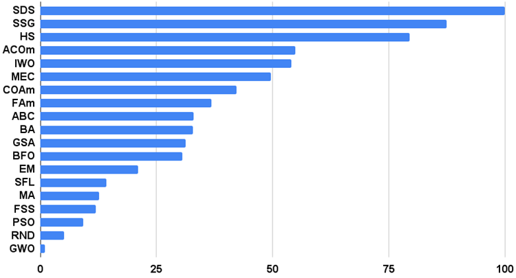
Figure 4. Histogram of the final results of testing algorithms

Pros and cons of the Stochastic Diffusion Search (SDS) algorithm:

Pros:
1. Minimum number of external parameters.
2. High efficiency in solving a variety of problems.
3. Low load on computing resources.
4. Ease of implementation.
5. Resistance to sticking.
6. Promising results on both smooth and complex discrete functions.
7. High convergence.

Cons:
1. Not found.

Each article features an archive that contains updated current versions of the algorithm codes for all previous articles. However, it should be noted that I am not responsible for absolute accuracy in the description of canonical algorithms. I often add my own ideas and improvements based on my experience and personal opinions. The conclusions and judgments presented in the articles are based on the results of the experiments.