Billiards Optimization Algorithm (BOA)

Contents

1. Introduction
2. Implementation of the algorithm
3. Test results

Introduction

In the world of optimization algorithms, where mathematical precision meets real-world inspiration, strikingly ingenious approaches are often born. One such method is the Billiards Optimization Algorithm (BOA), which draws ideas for a search strategy from the mechanics of the classic game of billiards.

Imagine a pool table where each pocket is a potential solution, and the balls are solution seekers moving through the space of possibilities. Just as a skilled billiard player calculates the trajectory of a ball to accurately pocket it, BOA guides its decisions toward optimal results through an iterative process of search and refinement. This algorithm, developed by researchers Hadi Givi and Marie Hubálovská in 2023, demonstrates an interesting and unusual approach to solving optimization problems.

In this article, we dive into the conceptual basis of BOA, explore its mathematical model, and analyze its efficiency in solving multimodal problems. The algorithm, which combines conceptual simplicity with mathematical precision, opens new horizons in the field of computational optimization and represents a valuable addition to the arsenal of modern optimization methods.

Implementation of the algorithm

The BOA algorithm is an optimization method inspired by the game of billiards. Imagine that you are looking for the best solution to some problem, in billiard terminology, it is like trying to get the ball into the pocket. There are 8 pockets on a pool table, as well as many balls. At the beginning of the algorithm, a group of random solutions (population) is created. These decisions are like balls on a pool table. For each solution, the objective function value is calculated to determine how good it is.

At each iteration of the algorithm, the eight best solutions from the population become "pockets" (targets to strive for). The remaining solutions are treated as balls that need to be directed towards these pockets. For each ball (solution), one of the pockets (best solutions) is randomly selected. The new position of the ball is then calculated - a new solution moving in the direction of the chosen pocket. If the new position of the ball gives a better value of the objective function, then the ball moves to the new position, and if not, then it remains in place.

Mathematically it looks like this:

X_new = X + rnd [0.0; 1.0] × (P - I × X)

where:

• X_new — new position of the ball,
• X — current position of the ball,
• P — position of the pocket (or the ball that the current ball is supposed to hit),
• I — random selection of numbers 1 or 2.

The process is repeated many times, and eventually the balls (solutions) should approach the optimal solution to the problem.

An advantage of BOA may lie in the fact that it should theoretically balance well, with just one coefficient in the equation, between global search and local search. This is achieved by using a random ratio I, which ensures either an "undershoot" of the ball (refining solutions near good points) or an "overshoot" (exploration of different areas of the solution space).

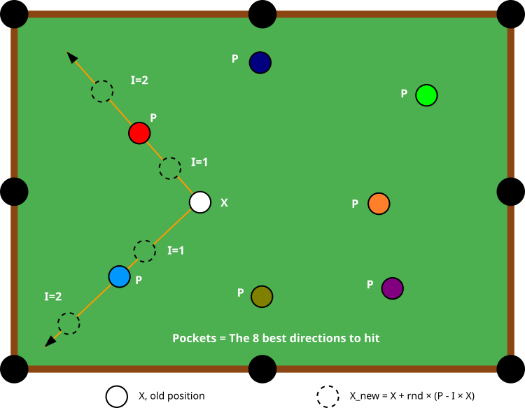
Figure 1. The BOA algorithm flow chart

Figure 1 schematically shows the operating principle of the BOA algorithm. The central element, a white ball marked "X", represents the agent's current position in the solution search space. Around this ball are colored balls marked "P" - these are "pockets" or "holes" representing the 8 best solutions found so far. The diagram demonstrates how an agent (the white ball) can update its position by moving towards different pockets, namely, for each step, the agent randomly chooses one of the eight pockets as the target direction of movement.

The orange lines with arrows show the possible trajectories of the agent's movement to different pockets (in this case, to the red and blue ones). The dotted circles represent intermediate positions that the agent can take while moving, depending on the value of I (1 or 2). The value of I changes the "strength of the blow" and the nature of the movement: at I=1, the position shifts in the direction of the selected pocket, and at I=2, the agent can make sharper movements, which facilitates the exploration of a larger part of the solution space.

Now that we have fully understood how the algorithm works, we will start writing BOA pseudocode.

Initialization
    Determine the number of balls (popSize) and pockets (numPockets).
    Create a population of balls (agents).
    Set the search space with minimum and maximum boundaries.

Basic algorithm
First stage: Initial initialization (performed only once)
    For each ball in the population:
        Randomly place balls in the search space.
        Save its initial position.
        Set the initial values of the fitness function to the minimum.

Second stage: Moving balls
    For each ball in the population:
        For each coordinate of the ball:
            Choose a random pocket (one of the numPockets best solutions).
            Update the position of the ball using the equation: X_new = X + rnd [0.0; 1.0] × (P - I × X)
            Check that the new position remains within acceptable limits.

Third stage: Update the best solutions
    For each ball:
        If the value of the ball fitness function is better than the global best, update the global best.
        If the value of the ball fitness function is better than its own best, update its best.
    Sort the balls by their best fitness function values.
        The first numPockets of agents after sorting become pockets for the next iteration.

Repeat the Ball movement and Best solution update steps until a stopping condition is reached (for example, the maximum number of iterations).

Let's start writing the algorithm code. The C_AO_BOA class is derived from the C_AO class (the base class of population optimization algorithms) and implements the BOA optimization algorithm. Let's take a look at its key elements:

The C_AO_BOA () constructor initializes the values of instance variables:

• popSize is set to 50, which represents the number of balls (agents) in the algorithm.
• numPockets is set to 8, it forms the number of pockets on a pool table.
• The params array size is changed and two parameters (popSize and numPockets) are added to the params array.

Methods:

• SetParams () — the method is responsible for setting the parameters from the 'params' array back into the local popSize and numPockets variables.
• Init () — initialization method configures the minimum, maximum values and steps for searching, as well as sets the number of epochs.
• Moving () — manages the movement of balls in the algorithm.
• Revision () — verifies and revises agents’ positions/decisions.

//——————————————————————————————————————————————————————————————————————————————
class C_AO_BOA : public C_AO
{
  public: //--------------------------------------------------------------------
  ~C_AO_BOA () { }
  C_AO_BOA ()
  {
    ao_name = "BOA";
    ao_desc = "Billiards Optimization Algorithm";
    ao_link = "https://www.mql5.com/en/articles/17325";

    popSize    = 50;  // number of balls (agents)
    numPockets = 8;   // number of pockets on a billiard table

    ArrayResize (params, 2);

    params [0].name = "popSize";    params [0].val = popSize;
    params [1].name = "numPockets"; params [1].val = numPockets;
  }

  void SetParams ()
  {
    popSize    = (int)params [0].val;
    numPockets = (int)params [1].val;
  }

  bool Init (const double &rangeMinP  [],  // minimum values
             const double &rangeMaxP  [],  // maximum values
             const double &rangeStepP [],  // step change
             const int     epochsP = 0);   // number of epochs

  void Moving   ();
  void Revision ();

  //----------------------------------------------------------------------------
  int numPockets;       // number of pockets (best solutions)

  private: //-------------------------------------------------------------------
};
//——————————————————————————————————————————————————————————————————————————————

The Init method in the C_AO_BOA class is responsible for initializing the BOA algorithm. At the beginning of the method, the StandardInit() function is called, passing arrays of minimum and maximum values, as well as steps to it. The function is responsible for performing common actions and initializations that must be performed for all derived classes of optimization algorithms (including initial range setup), as well as preparing the underlying search agents in the algorithm. If StandardInit () returns 'false' (initialization failed), the Init method also returns 'false'. If everything goes well, the method returns 'true'.

//——————————————————————————————————————————————————————————————————————————————
//--- Initialization
bool C_AO_BOA::Init (const double &rangeMinP  [],
                     const double &rangeMaxP  [],
                     const double &rangeStepP [],
                     const int epochsP = 0)
{
  if (!StandardInit (rangeMinP, rangeMaxP, rangeStepP)) return false;

  //----------------------------------------------------------------------------
  return true;
}
//——————————————————————————————————————————————————————————————————————————————

The Moving method implements the main step of the BOA algorithm and controls the movement of agents (balls) in the solution space. First, the if (!revision) condition is checked to determine whether the method is being called for the first time. If revision=false, agent positions need to be initialized. To do this, a loop is executed over all agents defined as popSize, within which a nested loop is executed over the coordinates that define the decision parameters of each agent.

At the stage of generating initial positions, a random value for each agent coordinate is selected in a given range, and the u.SeInDiSp() function brings the value to an acceptable value, taking into account the step. The agent's initial position is stored in a[p].cB[c] as the ball's best individual solution (on the first iteration, the initial solution is equivalent to the best known one), and after setting revision=true, the method terminates, preventing reinitialization of values.

On the second and subsequent iterations, a loop is started for all agents to move. During the coordinate update, nested loops are performed over all agents and their coordinates, where one of the best available pockets is randomly selected to update the agent's current position. The position is updated based on the previous position plus a random change based on the position of the selected pocket. The u.RNDprobab() function returns a random number in the range [0.0; 1.0] to add random noise, while the u.RNDintInRange(1, 2) function multiplies a random value of 1 or 2 with the agent's position.

After updating the position, it is adjusted, bringing the updated value to the specified range, taking into account the minimum and maximum values, as well as the change step.

//——————————————————————————————————————————————————————————————————————————————
//--- The main step of the algorithm
void C_AO_BOA::Moving ()
{
  //----------------------------------------------------------------------------
  // Initial initialization
  if (!revision)
  {
    for (int p = 0; p < popSize; p++)
    {
      for (int c = 0; c < coords; c++)
      {
        a [p].c  [c] = u.RNDfromCI (rangeMin [c], rangeMax [c]);
        a [p].c  [c] = u.SeInDiSp (a [p].c [c], rangeMin [c], rangeMax [c], rangeStep [c]);
        a [p].cB [c] = a [p].c [c];  // Save the initial position
      }
    }

    revision = true;
    return;
  }

  //----------------------------------------------------------------------------
  for (int p = 0; p < popSize; p++)
  {
    for (int c = 0; c < coords; c++)
    {
      int pocketID = u.RNDminusOne (numPockets);

      a [p].c [c] = a [p].cB [c] + u.RNDprobab () * (a [pocketID].cB [c] - u.RNDintInRange (1, 2) * a [p].cB [c]);
      a [p].c [c] = u.SeInDiSp (a [p].c [c], rangeMin [c], rangeMax [c], rangeStep [c]);
    }
  }
}
//——————————————————————————————————————————————————————————————————————————————

The Revision method is responsible for updating the best global solution in the BOA algorithm, and also updates the best individual solutions of the balls. At the end of the method, the balls are sorted according to their best individual solutions.

//——————————————————————————————————————————————————————————————————————————————
//--- Update the best solution taking into account greedy selection and the probability of making worse decisions
void C_AO_BOA::Revision ()
{
  int bestIND = -1;

  for (int i = 0; i < popSize; i++)
  {
    if (a [i].f > fB)
    {
      fB = a [i].f;
      bestIND = i;
    }

    if (a [i].f > a [i].fB)
    {
      a [i].fB = a [i].f;
      ArrayCopy (a [i].cB, a [i].c, 0, 0, WHOLE_ARRAY);
    }
  }

  if (bestIND != -1) ArrayCopy (cB, a [bestIND].c, 0, 0, WHOLE_ARRAY);

  S_AO_Agent aT []; ArrayResize (aT, popSize);
  u.Sorting_fB (a, aT, popSize);
}
//——————————————————————————————————————————————————————————————————————————————

Test results

Now let's see how the BOA algorithm works:

BOA|Billiards Optimization Algorithm|50.0|8.0|
=============================
5 Hilly's; Func runs: 10000; result: 0.63960620766331
25 Hilly's; Func runs: 10000; result: 0.3277725645995603
500 Hilly's; Func runs: 10000; result: 0.2514878043770147
=============================
5 Forest's; Func runs: 10000; result: 0.3885662762060409
25 Forest's; Func runs: 10000; result: 0.1955657530616877
500 Forest's; Func runs: 10000; result: 0.15336230733273673
=============================
5 Megacity's; Func runs: 10000; result: 0.5415384615384615
25 Megacity's; Func runs: 10000; result: 0.19046153846153846
500 Megacity's; Func runs: 10000; result: 0.10530769230769324
=============================
All score: 2.79367 (31.04%)

As you can see, the algorithm's performance is quite weak and it does not make it into our ranking table, so I decided to take a closer look at the algorithm and came up with some ideas on how to make it work. Let's look at the equation for the movement of balls again:

X_new = X + rnd [0.0; 1.0] × (P - I × X)

In this equation, the I ratio is applied to the value of the current coordinate of the ball, which has unclear physical meaning, since in fact the scaling is applied to the absolute value of the coordinate. The natural thing to do is to factor this ratio out to allow scaling to the difference between the pocket and the ball coordinate value. Then the resulting record describes a truly physical meaning, either the ball will not reach the pocket, or it will fly over it. The variability is provided by an additional noise factor of a random number in the range [0.0, 1.0].

As a result, we obtain the equation for the movement of balls:

X_new = X + rnd [0.0; 1.0] × (P -X) × I

So, below is the complete code for the modified version of the Moving () method, which shows the commented out string by author's equation followed by my equation version.

//——————————————————————————————————————————————————————————————————————————————
//--- The main step of the algorithm
void C_AO_BOA::Moving ()
{
  //----------------------------------------------------------------------------
  // Initial initialization
  if (!revision)
  {
    for (int p = 0; p < popSize; p++)
    {
      for (int c = 0; c < coords; c++)
      {
        a [p].c  [c] = u.RNDfromCI (rangeMin [c], rangeMax [c]);
        a [p].c  [c] = u.SeInDiSp (a [p].c [c], rangeMin [c], rangeMax [c], rangeStep [c]);
        a [p].cB [c] = a [p].c [c];  // Save the initial position as the best individual solution 
      }
    }

    revision = true;
    return;
  }

  //----------------------------------------------------------------------------
  for (int p = 0; p < popSize; p++)
  {
    for (int c = 0; c < coords; c++)
    {
      int pocketID = u.RNDminusOne (numPockets);

      //a [p].c [c] = a [p].cB [c] + u.RNDprobab () * (a [pocketID].cB [c] - u.RNDintInRange (1, 2) * a [p].cB [c]);
      a [p].c [c] = a [p].cB [c] + u.RNDprobab () * (a [pocketID].cB [c] - a [p].cB [c]) * u.RNDintInRange (1, 2);
      a [p].c [c] = u.SeInDiSp (a [p].c [c], rangeMin [c], rangeMax [c], rangeStep [c]);
    }
  }
}
//——————————————————————————————————————————————————————————————————————————————

Now, after the changes, let's see how the algorithm works with the parameters the authors' version showed the best results with:

BOA|Billiards Optimization Algorithm|50.0|8.0|
=============================
5 Hilly's; Func runs: 10000; result: 0.8727603657603271
25 Hilly's; Func runs: 10000; result: 0.7117647027521633
500 Hilly's; Func runs: 10000; result: 0.25339119302510993
=============================
5 Forest's; Func runs: 10000; result: 0.9228482722678735
25 Forest's; Func runs: 10000; result: 0.7601448268715335
500 Forest's; Func runs: 10000; result: 0.3498925749480034
=============================
5 Megacity's; Func runs: 10000; result: 0.6184615384615385
25 Megacity's; Func runs: 10000; result: 0.45876923076923076
500 Megacity's; Func runs: 10000; result: 0.14586153846153965
=============================
All score: 5.09389 (56.60%)

After conducting a few more experiments, I came up with parameters that produced even better results:

BOA|Billiards Optimization Algorithm|50.0|25.0|
=============================
5 Hilly's; Func runs: 10000; result: 0.957565927297626
25 Hilly's; Func runs: 10000; result: 0.8259872884790693
500 Hilly's; Func runs: 10000; result: 0.2523458952211869
=============================
5 Forest's; Func runs: 10000; result: 0.9999999999999929
25 Forest's; Func runs: 10000; result: 0.900362056289584
500 Forest's; Func runs: 10000; result: 0.305018130407844
=============================
5 Megacity's; Func runs: 10000; result: 0.7353846153846153
25 Megacity's; Func runs: 10000; result: 0.5252307692307692
500 Megacity's; Func runs: 10000; result: 0.09563076923077005
=============================
All score: 5.59753 (62.19%)

Let's look at the visualization of the BOA algorithm running on test functions. No particular characteristic behavior is observed in the search space; the movements of the "balls" appear chaotic. It is particularly striking that the algorithm successfully copes with problems of small and medium dimensions, however, large dimension problems show convergence issues. This is especially noticeable on the smooth Hilly function, where the performance is even worse than on the discrete Megacity, which is an extremely rare phenomenon compared to other population-based algorithms. It is also worth noting the algorithm's tendency to get stuck in local minima when solving small dimension problems.

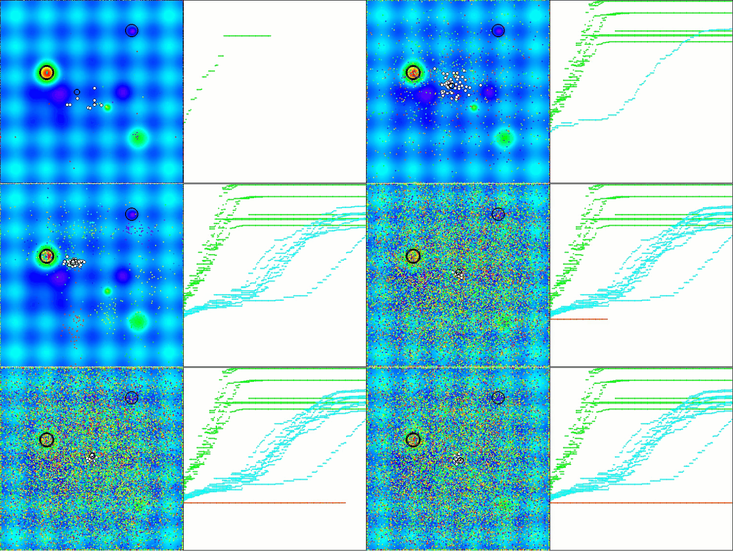
BOA on the Hilly test function

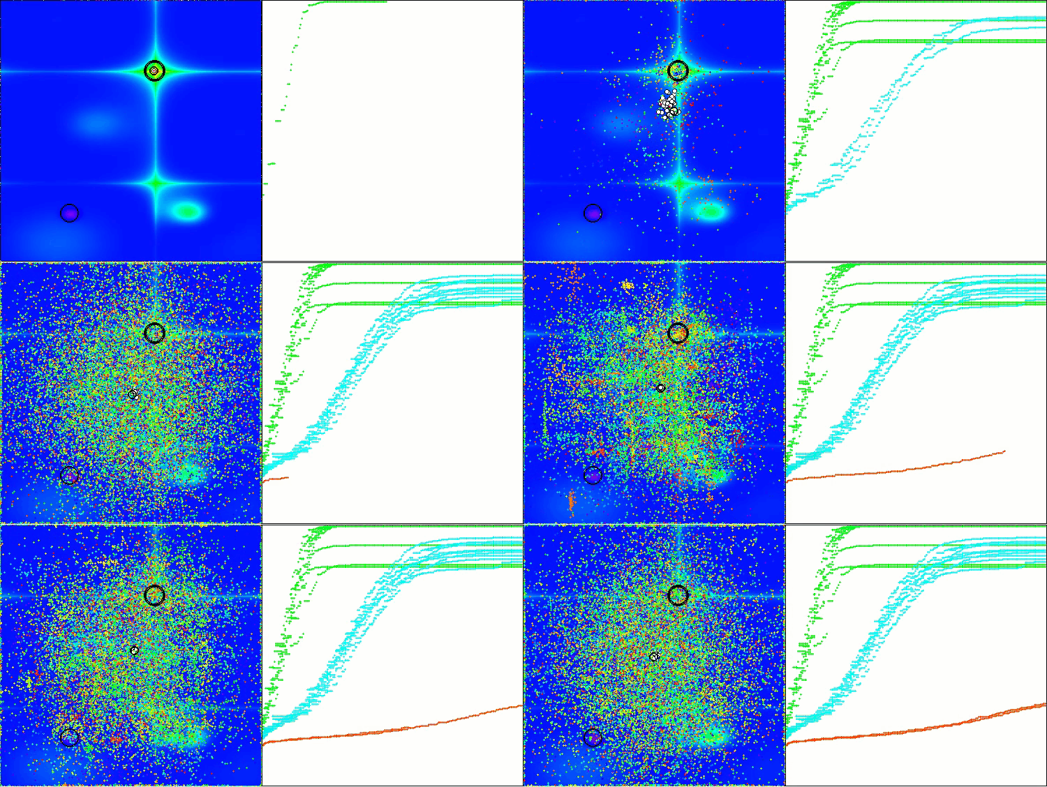
BOA on the Forest test function

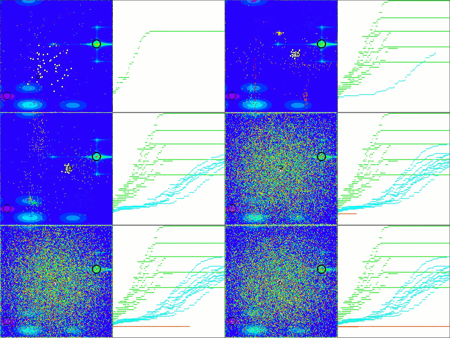
BOA on the Megacity test function

Let's summarize the test results and look at the efficiency. The algorithm turned out to be quite efficient taking the 8th place in the ranking of the best optimization algorithms, despite having serious shortcomings.

#	AO	Description	Hilly			Hilly final	Forest			Forest final	Megacity (discrete)			Megacity final	Final result	% of MAX
			10 p (5 F)	50 p (25 F)	1000 p (500 F)		10 p (5 F)	50 p (25 F)	1000 p (500 F)		10 p (5 F)	50 p (25 F)	1000 p (500 F)
1	ANS	across neighbourhood search	0.94948	0.84776	0.43857	2.23581	1.00000	0.92334	0.39988	2.32323	0.70923	0.63477	0.23091	1.57491	6.134	68.15
2	CLA	code lock algorithm (joo)	0.95345	0.87107	0.37590	2.20042	0.98942	0.91709	0.31642	2.22294	0.79692	0.69385	0.19303	1.68380	6.107	67.86
3	AMOm	animal migration ptimization M	0.90358	0.84317	0.46284	2.20959	0.99001	0.92436	0.46598	2.38034	0.56769	0.59132	0.23773	1.39675	5.987	66.52
4	(P+O)ES	(P+O) evolution strategies	0.92256	0.88101	0.40021	2.20379	0.97750	0.87490	0.31945	2.17185	0.67385	0.62985	0.18634	1.49003	5.866	65.17
5	CTA	comet tail algorithm (joo)	0.95346	0.86319	0.27770	2.09435	0.99794	0.85740	0.33949	2.19484	0.88769	0.56431	0.10512	1.55712	5.846	64.96
6	TETA	time evolution travel algorithm (joo)	0.91362	0.82349	0.31990	2.05701	0.97096	0.89532	0.29324	2.15952	0.73462	0.68569	0.16021	1.58052	5.797	64.41
7	SDSm	stochastic diffusion search M	0.93066	0.85445	0.39476	2.17988	0.99983	0.89244	0.19619	2.08846	0.72333	0.61100	0.10670	1.44103	5.709	63.44
8	BOAm	billiards optimization algorithm M	0.95757	0.82599	0.25235	2.03590	1.00000	0.90036	0.30502	2.20538	0.73538	0.52523	0.09563	1.35625	5.598	62.19
9	AAm	archery algorithm M	0.91744	0.70876	0.42160	2.04780	0.92527	0.75802	0.35328	2.03657	0.67385	0.55200	0.23738	1.46323	5.548	61.64
10	ESG	evolution of social groups (joo)	0.99906	0.79654	0.35056	2.14616	1.00000	0.82863	0.13102	1.95965	0.82333	0.55300	0.04725	1.42358	5.529	61.44
11	SIA	simulated isotropic annealing (joo)	0.95784	0.84264	0.41465	2.21513	0.98239	0.79586	0.20507	1.98332	0.68667	0.49300	0.09053	1.27020	5.469	60.76
12	ACS	artificial cooperative search	0.75547	0.74744	0.30407	1.80698	1.00000	0.88861	0.22413	2.11274	0.69077	0.48185	0.13322	1.30583	5.226	58.06
13	DA	dialectical algorithm	0.86183	0.70033	0.33724	1.89940	0.98163	0.72772	0.28718	1.99653	0.70308	0.45292	0.16367	1.31967	5.216	57.95
14	BHAm	black hole algorithm M	0.75236	0.76675	0.34583	1.86493	0.93593	0.80152	0.27177	2.00923	0.65077	0.51646	0.15472	1.32195	5.196	57.73
15	ASO	anarchy society optimization	0.84872	0.74646	0.31465	1.90983	0.96148	0.79150	0.23803	1.99101	0.57077	0.54062	0.16614	1.27752	5.178	57.54
16	RFO	royal flush optimization (joo)	0.83361	0.73742	0.34629	1.91733	0.89424	0.73824	0.24098	1.87346	0.63154	0.50292	0.16421	1.29867	5.089	56.55
17	AOSm	atomic orbital search M	0.80232	0.70449	0.31021	1.81702	0.85660	0.69451	0.21996	1.77107	0.74615	0.52862	0.14358	1.41835	5.006	55.63
18	TSEA	turtle shell evolution algorithm (joo)	0.96798	0.64480	0.29672	1.90949	0.99449	0.61981	0.22708	1.84139	0.69077	0.42646	0.13598	1.25322	5.004	55.60
19	DE	differential evolution	0.95044	0.61674	0.30308	1.87026	0.95317	0.78896	0.16652	1.90865	0.78667	0.36033	0.02953	1.17653	4.955	55.06
20	CRO	chemical reaction optimization	0.94629	0.66112	0.29853	1.90593	0.87906	0.58422	0.21146	1.67473	0.75846	0.42646	0.12686	1.31178	4.892	54.36
21	BIO	blood inheritance optimization (joo)	0.81568	0.65336	0.30877	1.77781	0.89937	0.65319	0.21760	1.77016	0.67846	0.47631	0.13902	1.29378	4.842	53.80
22	BSA	bird swarm algorithm	0.89306	0.64900	0.26250	1.80455	0.92420	0.71121	0.24939	1.88479	0.69385	0.32615	0.10012	1.12012	4.809	53.44
23	HS	harmony search	0.86509	0.68782	0.32527	1.87818	0.99999	0.68002	0.09590	1.77592	0.62000	0.42267	0.05458	1.09725	4.751	52.79
24	SSG	saplings sowing and growing	0.77839	0.64925	0.39543	1.82308	0.85973	0.62467	0.17429	1.65869	0.64667	0.44133	0.10598	1.19398	4.676	51.95
25	BCOm	bacterial chemotaxis optimization M	0.75953	0.62268	0.31483	1.69704	0.89378	0.61339	0.22542	1.73259	0.65385	0.42092	0.14435	1.21912	4.649	51.65
26	ABO	african buffalo optimization	0.83337	0.62247	0.29964	1.75548	0.92170	0.58618	0.19723	1.70511	0.61000	0.43154	0.13225	1.17378	4.634	51.49
27	(PO)ES	(PO) evolution strategies	0.79025	0.62647	0.42935	1.84606	0.87616	0.60943	0.19591	1.68151	0.59000	0.37933	0.11322	1.08255	4.610	51.22
28	TSm	tabu search M	0.87795	0.61431	0.29104	1.78330	0.92885	0.51844	0.19054	1.63783	0.61077	0.38215	0.12157	1.11449	4.536	50.40
29	BSO	brain storm optimization	0.93736	0.57616	0.29688	1.81041	0.93131	0.55866	0.23537	1.72534	0.55231	0.29077	0.11914	0.96222	4.498	49.98
30	WOAm	wale optimization algorithm M	0.84521	0.56298	0.26263	1.67081	0.93100	0.52278	0.16365	1.61743	0.66308	0.41138	0.11357	1.18803	4.476	49.74
31	AEFA	artificial electric field algorithm	0.87700	0.61753	0.25235	1.74688	0.92729	0.72698	0.18064	1.83490	0.66615	0.11631	0.09508	0.87754	4.459	49.55
32	AEO	artificial ecosystem-based optimization algorithm	0.91380	0.46713	0.26470	1.64563	0.90223	0.43705	0.21400	1.55327	0.66154	0.30800	0.28563	1.25517	4.454	49.49
33	ACOm	ant colony optimization M	0.88190	0.66127	0.30377	1.84693	0.85873	0.58680	0.15051	1.59604	0.59667	0.37333	0.02472	0.99472	4.438	49.31
34	BFO-GA	bacterial foraging optimization - ga	0.89150	0.55111	0.31529	1.75790	0.96982	0.39612	0.06305	1.42899	0.72667	0.27500	0.03525	1.03692	4.224	46.93
35	SOA	simple optimization algorithm	0.91520	0.46976	0.27089	1.65585	0.89675	0.37401	0.16984	1.44060	0.69538	0.28031	0.10852	1.08422	4.181	46.45
36	ABHA	artificial bee hive algorithm	0.84131	0.54227	0.26304	1.64663	0.87858	0.47779	0.17181	1.52818	0.50923	0.33877	0.10397	0.95197	4.127	45.85
37	ACMO	atmospheric cloud model optimization	0.90321	0.48546	0.30403	1.69270	0.80268	0.37857	0.19178	1.37303	0.62308	0.24400	0.10795	0.97503	4.041	44.90
38	ADAMm	adaptive moment estimation M	0.88635	0.44766	0.26613	1.60014	0.84497	0.38493	0.16889	1.39880	0.66154	0.27046	0.10594	1.03794	4.037	44.85
39	CGO	chaos game optimization	0.57256	0.37158	0.32018	1.26432	0.61176	0.61931	0.62161	1.85267	0.37538	0.21923	0.19028	0.78490	3.902	43.35
40	ATAm	artificial tribe algorithm M	0.71771	0.55304	0.25235	1.52310	0.82491	0.55904	0.20473	1.58867	0.44000	0.18615	0.09411	0.72026	3.832	42.58
41	ASHA	artificial showering algorithm	0.89686	0.40433	0.25617	1.55737	0.80360	0.35526	0.19160	1.35046	0.47692	0.18123	0.09774	0.75589	3.664	40.71
42	ASBO	adaptive social behavior optimization	0.76331	0.49253	0.32619	1.58202	0.79546	0.40035	0.26097	1.45677	0.26462	0.17169	0.18200	0.61831	3.657	40.63
43	MEC	mind evolutionary computation	0.69533	0.53376	0.32661	1.55569	0.72464	0.33036	0.07198	1.12698	0.52500	0.22000	0.04198	0.78698	3.470	38.55
44	CSA	circle search algorithm	0.66560	0.45317	0.29126	1.41003	0.68797	0.41397	0.20525	1.30719	0.37538	0.23631	0.10646	0.71815	3.435	38.17
45	IWO	invasive weed optimization	0.72679	0.52256	0.33123	1.58058	0.70756	0.33955	0.07484	1.12196	0.42333	0.23067	0.04617	0.70017	3.403	37.81
	RW	random walk	0.48754	0.32159	0.25781	1.06694	0.37554	0.21944	0.15877	0.75375	0.27969	0.14917	0.09847	0.52734	2.348	26.09

Summary

The modified billiard optimization algorithm (BOAm) showed interesting results on test functions. Analysis of the presented data shows that the algorithm achieves the best results on small and medium-sized problems, gaining maximum values in the Hilly (0.957), Forest (0.999) and Megacity (0.735) tests when reaching 10,000 iterations. This demonstrates its high efficiency in finding optimal solutions for problems of moderate complexity. However, performance drops significantly as the problem size increases, as seen in the results for the 1000-variable scenarios, where the scores drop to 0.252, 0.305, and 0.095, respectively.

It is especially important to note the significant performance improvement in the modified version of the algorithm, which achieves 62.19% of the maximum possible result, which is double the original version's 31.04%. This impressive improvement was achieved by changing just one line of code, which concerns the equation for updating the balls' positions.

The simplicity of the algorithm is both its advantage and its limitation — it is intuitive, easy to implement, and based on an elegant billiards concept — but may require additional modifications to handle high-dimensional problems efficiently. Overall, ranking in the top ten algorithms of the ranking table, BOAm represents a promising metaheuristic approach with a good balance between exploration and exploitation of the solution space.

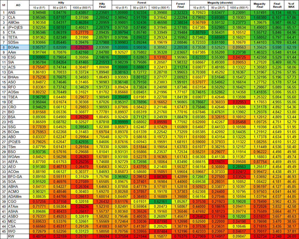
Figure 2. Color gradation of algorithms according to the corresponding tests

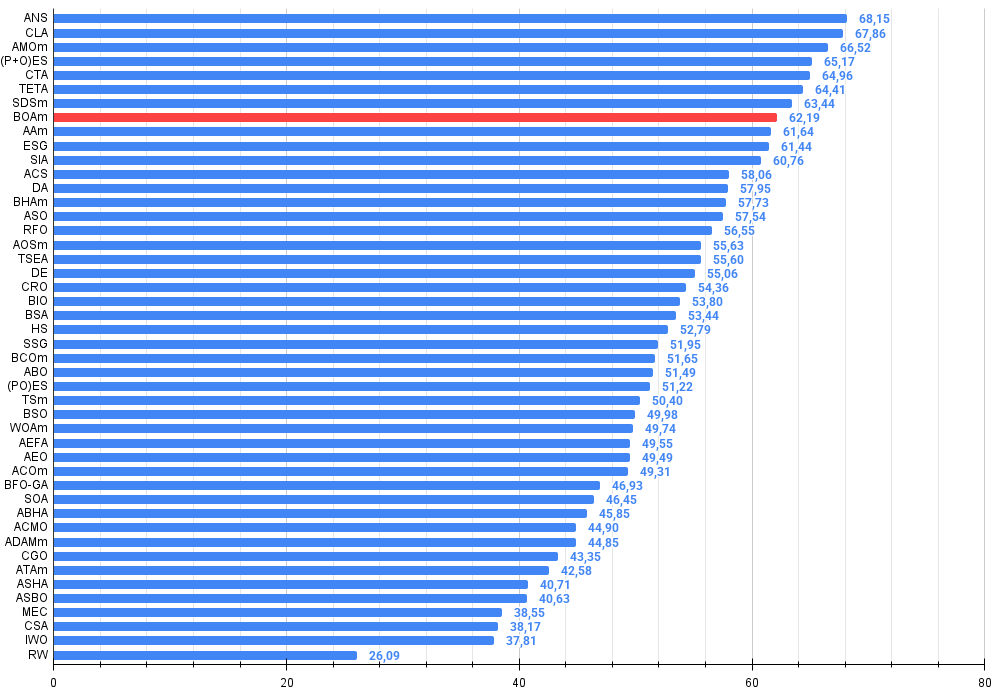
Figure 3. Histogram of algorithm testing results (scale from 0 to 100, the higher the better, where 100 is the maximum possible theoretical result, in the archive there is a script for calculating the rating table)

BOA pros and cons:

Pros:

1. Very few external parameters.
2. Simple implementation.
   
3. Performs well on small and medium-sized problems.
4. Excellent results on problems with "sharp" extremes (such as the Forest function).
   

Cons:

1. Gets stuck at local extremes on low-dimensional problems.
   
2. Very low speed and accuracy of convergence on "smooth" problems (such as the Hilly function) of high dimension.

The article is accompanied by an archive with the current versions of the algorithm codes. The author of the article is not responsible for the absolute accuracy in the description of canonical algorithms. Changes have been made to many of them to improve search capabilities. The conclusions and judgments presented in the articles are based on the results of the experiments.

• github: https://github.com/JQSakaJoo/Population-optimization-algorithms-MQL5

Programs used in the article

#	Name	Type	Description
1	#C_AO.mqh	Include	Parent class of population optimization algorithms
2	#C_AO_enum.mqh	Include	Enumeration of population optimization algorithms
3	TestFunctions.mqh	Include	Library of test functions
4	TestStandFunctions.mqh	Include	Test stand function library
5	Utilities.mqh	Include	Library of auxiliary functions
6	CalculationTestResults.mqh	Include	Script for calculating results in the comparison table
7	Testing AOs.mq5	Script	The unified test stand for all population optimization algorithms
8	Simple use of population optimization algorithms.mq5	Script	A simple example of using population optimization algorithms without visualization
9	Test_AO_BOAm.mq5	Script	BOAm test stand