
Across Neighbourhood Search (ANS)
1. Introduction
In today's world, developing efficient optimization methods plays an important role in solving a variety of problems, ranging from engineering applications to scientific research in the field of machine learning and artificial intelligence. In this context, metaheuristic evolutionary algorithms represent powerful tools for solving complex optimization problems. However, to further improve their performance and efficiency, continuous development and modification of existing methods, as well as the development of new algorithms, is necessary.
In this article, I will introduce an optimization algorithm known as Across Neighborhood Search (ANS), proposed by Guohua Wu in 2014, which is based on population search for numerical optimization. The developed ANS algorithm represents a significant step forward in the field of optimization, promising to solve various problems in the real world with high efficiency and accuracy. We will if it is true below. The basic idea of ANS is to model the behavior of a multi-agent system, where each agent moves through a solution space, interacting with its neighbors and exchanging information. This approach allows for excellent exploration of the search space by combining local and global optimization.
We will get acquainted with a detailed description of the structure of the ANS algorithm and the principles of its operation, and also conduct a comparative analysis with existing optimization methods. The developed ANS algorithm opens up the field of optimization, allowing us to solve a wide range of problems with high performance. Moreover, in the context of the development of artificial intelligence, it is important to note that the ANS algorithm represents an important step towards creating more flexible and intelligent optimization methods that can take into account the specifics of the problem and the dynamics of the environment.
2. Implementation of the algorithm
Across Neighborhood Search (ANS) algorithm is an optimization method that uses ideas from the field of evolutionary algorithms and metaheuristics and is designed to find optimal solutions in the problem parameters space.
Let us note the main features of ANS:
- Neighborhood search - agents explore the neighborhoods of current solutions, which allows them to find local optima more efficiently.
- Using the normal distribution - ANS uses the normal distribution to generate new parameter values.
- Solution Collections - ANS uses collections of best solutions that help to orient the algorithm in several promising directions at once.
In ANS, a group of individuals jointly searches a solution space to optimally solve the optimization problem under consideration. The basic idea of the algorithm is to maintain and dynamically update a collection of excellent solutions found by individuals so far. In each generation, the individual directly searches the neighborhood for several distinct solutions according to the normal probability distribution. In this way, the idea of having several potentially good solutions at once is exploited, since it is not known in advance which of them will be the best.
Below we will consider a complete description of the ANS algorithm with equations and stages, according to the author's concept. ANS performs the following steps:
1. Initialization of parameters:
- Population size m
- Collection of the best solutions set c
- Standard deviation of a Gaussian distribution sigma
- Search space dimensionality D
- Maximum number of generations MaxG
2. Initialization of the population. Random initialization of the position of each individual in the population in the search space.
3. Updating the best solutions. Each individual in the population updates its current position by exploring the neighborhood of the best solutions from the collection using the normal distribution.
4. Select coordinates for search. n random number selection (across-search degree) to determine the current coordinate of the individual's position in the solution space.
5. Updating the position of an individual. Updating the position of an individual i according to the previous step.
Equations and operations:
1. Updating position pos_i of the i individual (exploring the neighborhood of a solution from a collection):
- Position of the individual i is updated using a Gaussian distribution: pos_i = r_g + G (r_g - pos_i), where:
- G - random value from a Gaussian distribution
- r_g - position of the best solution from the collection
2. Updating position pos_i of the i individual (exploring the neighborhood of the individual's own best solution):
- Position of the individual i is updated using a Gaussian distribution: pos_i = r_i + G (r_i - pos_i), where:
- G - random value from a Gaussian distribution
- r_i - position of the individual's best solution
3. Updating a set of the best solutions:
- The collection of the best solutions is updated based on new positions of individuals.
Thus, the equations reflect the mechanism of searching for the i individual in the neighborhood of its best solution r_i, as well as in the neighborhood of other best solutions r_g from the R collection. These steps of the algorithm represent the basic logic of the ANS (Across Neighbourhood Search) method for solving optimization problems. It includes initialization of parameters, random initialization of individual positions, updating individual positions given the neighborhoods of the best solutions, and updating the collection of best solutions. The algorithm continues to run until the stop condition is met.
Search based on best solutions or individuals is a common and frequently used search method in population strategy algorithms, although the processes implementing such a search mechanism may differ for different optimization algorithms. In this case, a new population is introduced in addition to the main population of agents - a collection of the best solutions (potential search directions). The collection size is defined in the external parameters of the algorithm and can be set either smaller or larger than the size of the main population.
The search strategy in the ANS algorithm starts with filling the collection of best solutions and moves on to searching in the neighborhood of the best solutions of the collection and the best individual solutions of each agent. The size of the standard deviation sigma plays a key role in the algorithm. Low sigma provides a broader exploration of the search space, while higher values provide a refinement of solutions by narrowing their neighborhood. This algorithm parameter is responsible for the balance between search intensification and diversification. Some algorithms tie this balance to the current epoch number to allow dynamic changes in the balance between exploration and refinement, but in this case the authors defined the balance adjustment as an external parameter of ANS.
Thus, the ANS algorithm combines the exploitation of the best found solutions (through searching in their neighborhoods) and the exploration of the solution space (through searching in the neighborhoods of individuals' own best solutions). This should theoretically provide a good balance between search intensification and diversification.
Now let's move on to writing and parsing the ANS algorithm code. Define the S_ANS_Agent structure, which will be used to represent agents in the ANS algorithm. Structure fields:
- c - array for storing agent coordinates.
- cBest - array for storing the best agent coordinates.
- f - agent fitness value.
- fBest - best agent fitness value.
- Init(int coords) - initialization method, which sets the sizes of c and cBest arrays and sets the initial f and fBest values.
This part of the code represents the basic structure of an agent. The array of agents will represent the main population in the ANS algorithm.
//——————————————————————————————————————————————————————————————————————————————
struct S_ANS_Agent
{
    double c     []; //coordinates
    double cBest []; //best coordinates
    double f;        //fitness
    double fBest;    //best fitness

    void Init (int coords)
    {
      ArrayResize (c,     coords);
      ArrayResize (cBest, coords);
      f     = -DBL_MAX;
      fBest = -DBL_MAX;
    }
};
//—————————————————————————————————————————————————————————————————————————————
To describe a collection of the best solutions, set the structure S_Collection, which will be used to store information about the best coordinates in the search space and the corresponding fitness value. The structure contains the following fields:
- c - array for storing coordinates.
- f - fitness value for a given solution to a problem in the collection.
- Init(int coords) - initialization method sets the size of the c arrays and the initial f value to the minimum possible value of the double type.
//——————————————————————————————————————————————————————————————————————————————
struct S_Collection
{
    double c []; //coordinates
    double f;    //fitness

    void Init (int coords)
    {
      ArrayResize (c, coords);
      f = -DBL_MAX;
    }
};
//——————————————————————————————————————————————————————————————————————————————
Declare the C_AO_ANS class, which is an inheritor of the C_AO base class and is an implementation of the Across Neighbourhood Search (ANS) algorithm. Here are some key points:
- ao_name, ao_desc, ao_link - properties describing the ANS algorithm.
- popSize - population size.
- collectionSize, sigma, range, collChoiceProbab - ANS algorithm parameters.
- SetParams() - method for setting parameters.
- Init(), Moving(), Revision() - methods for initializing, moving agents, and updating the population and solution collection.
- S_ANS_Agent, S_Collection - structures for storing agent data and collections.
//——————————————————————————————————————————————————————————————————————————————
class C_AO_ANS : public C_AO
{
  public: //--------------------------------------------------------------------
  ~C_AO_ANS () { }
  C_AO_ANS ()
  {
    ao_name = "ANS";
    ao_desc = "Across Neighbourhood Search";
    ao_link = "https://www.mql5.com/en/articles/15049";

    popSize          = 50;   //population size

    collectionSize   = 20;   //Best solutions collection
    sigma            = 3.0;  //Form of normal distribution
    range            = 0.5;  //Range of values dispersed
    collChoiceProbab = 0.8;  //Collection choice probab

    ArrayResize (params, 5);

    params [0].name = "popSize";          params [0].val = popSize;
    params [1].name = "collectionSize";   params [1].val = collectionSize;
    params [2].name = "sigma";            params [2].val = sigma;
    params [3].name = "range";            params [3].val = range;
    params [4].name = "collChoiceProbab"; params [4].val = collChoiceProbab;
  }

  void SetParams ()
  {
    popSize          = (int)params [0].val;
    collectionSize   = (int)params [1].val;
    sigma            = params      [2].val;
    range            = params      [3].val;
  }

  bool Init (const double &rangeMinP  [], //minimum search range
             const double &rangeMaxP  [], //maximum search range
             const double &rangeStepP [], //step search
             const int     epochsP = 0);  //number of epochs

  void Moving   ();
  void Revision ();

  //----------------------------------------------------------------------------
  int    collectionSize;    //Best solutions collection
  double sigma;             //Form of normal distribution
  double range;             //Range of values dispersed
  double collChoiceProbab;  //Collection choice probab

  S_ANS_Agent agent [];

  private: //-------------------------------------------------------------------
  S_Collection coll     [];
  S_Collection collTemp [];
};
//——————————————————————————————————————————————————————————————————————————————
The Init method initializes the parameters of the ANS algorithm.
- rangeMinP, rangeMaxP, rangeStepP - arrays representing the minimum, maximum, and step of the search range.
- epochsP - number of epochs (generations).
Inside the method:
- The successful initialization of the standard parameters is checked using StandardInit.
- Agent (agent) and collection (coll) arrays are created (second population for storing the best solutions), as well as collTemp (temporary array for sorting the collection).
- For each agent and collection, the Init method is called to set the initial values.
This method plays an important role in preparing the ANS algorithm to perform optimization. It is important to note that the coll and collTemp arrays are initialized with double the size relative to the collectionSize parameter. This is done so that new agents added to the collection end up in the second half of the array. Subsequent sorting occurs across the entire collection, and only the first half, containing the best agents, is used for further work.
//——————————————————————————————————————————————————————————————————————————————
bool C_AO_ANS::Init (const double &rangeMinP  [], //minimum search range
                     const double &rangeMaxP  [], //maximum search range
                     const double &rangeStepP [], //step search
                     const int     epochsP = 0)   //number of epochs
{
  if (!StandardInit (rangeMinP, rangeMaxP, rangeStepP)) return false;

  //----------------------------------------------------------------------------
  ArrayResize (agent, popSize);
  for (int i = 0; i < popSize; i++) agent [i].Init (coords);

  ArrayResize (coll,     collectionSize * 2);
  ArrayResize (collTemp, collectionSize * 2);
  for (int i = 0; i < collectionSize * 2; i++)
  {
    coll     [i].Init (coords);
    collTemp [i].Init (coords);
  }

  return true;
}
//——————————————————————————————————————————————————————————————————————————————
The Moving method performs the movement (displacement) of agents in the ANS algorithm. Let's take a closer look at this code:
1. Initialization (if revision is equal to false):
- If this is the first step (first epoch), then for each agent:
- The val random value is generated in the range from rangeMin[c] to rangeMax[c].
- The SeInDiSp operator is applied to take into account the step rangeStep[c].
- The val value is assigned to the agent[i].c[c] agent coordinates.
- The val value is also assigned to the best coordinates of the agent[i].cBest[c] agent (at this stage the fitness values of the agents are unknown, so the best coordinates are equal to the current initial ones).
- The val value is assigned to the a[i].c[c] agent array.
2. Moving agents (if revision equals to true):
- For each agent and each coordinate:
- If the random number is less than collChoiceProbab, a random solution is selected from the collection:
- The random index ind is selected from the collection (until a non-empty solution is found).
- The p value is taken from the current agent coordinates.
- The r value is taken from the selected solution from the collection.
- Otherwise, the best agent coordinates are used:
- The p value is taken from the current agent coordinates.
- The r value is taken from the best agent coordinates.
- The dist distance and the (min and max) range are calculated for movement.
- The min and max values are limited to the rangeMin[c] and rangeMax[c] ranges.
- The normal distribution with the r, min, max and sigma parameters.
- The val value is assigned to the agent[i].c[c] agent coordinates.
- The val value is also assigned to the a[i].c[c] agent array.
This code updates the coordinates of agents in the ANS algorithm, taking into account the best coordinates of agents and solutions in the collection.
//——————————————————————————————————————————————————————————————————————————————
void C_AO_ANS::Moving ()
{
  double val = 0.0;

  //----------------------------------------------------------------------------
  if (!revision)
  {
    for (int i = 0; i < popSize; i++)
    {
      for (int c = 0; c < coords; c++)
      {
        val = u.RNDfromCI (rangeMin [c], rangeMax [c]);
        val = u.SeInDiSp  (val, rangeMin [c], rangeMax [c], rangeStep [c]);

        agent [i].c     [c] = val;
        agent [i].cBest [c] = val;

        a [i].c [c] = val;
      }
    }

    revision = true;
    return;
  }

  //----------------------------------------------------------------------------
  double min  = 0.0;
  double max  = 0.0;
  double dist = 0.0;
  int    ind  = 0;
  double r    = 0.0;
  double p    = 0.0;

  for (int i = 0; i < popSize; i++)
  {
    for (int c = 0; c < coords; c++)
    {
      if (u.RNDprobab () < collChoiceProbab)
      {
        do ind = u.RNDminusOne (collectionSize);
        while (coll [ind].f == -DBL_MAX);

        p = agent [i].c   [c];
        r = coll  [ind].c [c];

      }
      else
      {
        p = agent [i].c     [c];
        r = agent [i].cBest [c];
      }

      dist = fabs (p - r) * range;
      min  = r - dist;
      max  = r + dist;

      if (min < rangeMin [c]) min = rangeMin [c];
      if (max > rangeMax [c]) max = rangeMax [c];

      val = u.GaussDistribution (r, min, max, sigma);
      val = u.SeInDiSp (val, rangeMin [c], rangeMax [c], rangeStep [c]);

      agent [i].c [c] = val;
      a     [i].c [c] = val;
    }
  }
}
//——————————————————————————————————————————————————————————————————————————————
The Revision method performs revision (update) of agents and collections in the ANS algorithm. Here are the main points:
- The first part of the method: searches for an agent whose fitness is better than the global solution with fitness fB and saves its coordinates into the array cB.
- The second part of the method: updates the best coordinates of the agents agent[i].cBest based on their current fitness a[i].f.
- The third part of the method: updates the coll collection based on the best coordinates of agents.
- Sort the collection.
This method plays an important role in updating agents and the solution collection during the execution of the algorithm. The population of agents is placed in the second part of the collection, the collection is sorted, and the first half of the collection containing the best solutions is then used.
//——————————————————————————————————————————————————————————————————————————————
void C_AO_ANS::Revision ()
{
  //----------------------------------------------------------------------------
  int ind = -1;

  for (int i = 0; i < popSize; i++)
  {
    if (a [i].f > fB)
    {
      fB = a [i].f;
      ind = i;
    }
  }

  if (ind != -1) ArrayCopy (cB, a [ind].c, 0, 0, WHOLE_ARRAY);

  //----------------------------------------------------------------------------
  for (int i = 0; i < popSize; i++)
  {
    if (a [i].f > agent [i].fBest)
    {
      agent [i].fBest = a [i].f;
      ArrayCopy (agent [i].cBest, a [i].c, 0, 0, WHOLE_ARRAY);
    }
  }

  //----------------------------------------------------------------------------
  int cnt = 0;
  for (int i = collectionSize; i < collectionSize * 2; i++)
  {
    if (cnt < popSize)
    {
      coll [i].f = agent [cnt].fBest;
      ArrayCopy (coll [i].c, agent [cnt].cBest, 0, 0, WHOLE_ARRAY);
      cnt++;
    }
    else break;
  }

  u.Sorting (coll, collTemp, collectionSize * 2);
}
//——————————————————————————————————————————————————————————————————————————————
3. Test results
ANS test stand results:
ANS|Across Neighbourhood Search|50.0|100.0|8.0|1.0|0.6|
=============================
5 Hilly's; Func runs: 10000; result: 0.9494753644543816
25 Hilly's; Func runs: 10000; result: 0.8477633752716718
500 Hilly's; Func runs: 10000; result: 0.43857039929159747
=============================
5 Forest's; Func runs: 10000; result: 0.9999999999988883
25 Forest's; Func runs: 10000; result: 0.9233446583489741
500 Forest's; Func runs: 10000; result: 0.3998822848099108
=============================
5 Megacity's; Func runs: 10000; result: 0.709230769230769
25 Megacity's; Func runs: 10000; result: 0.6347692307692309
500 Megacity's; Func runs: 10000; result: 0.2309076923076936
=============================
All score: 6.13394 (68.15%)
ANS shows impressive results on all test functions. Let's have a look at the visualization of this algorithm's operation on the test stand. The results of ANS are truly amazing, but some questions arise when visualizing. In particular, the behavior of the population is striking - it seems to disappear from sight. The solution space is cleared and the function landscape is left without agents. This can only mean one thing - despite the excellent results of the algorithm, the population is prone to degeneration. The collection of excellent solutions becomes cluttered with very similar solutions, and new solutions simply cannot be created because all solutions are derivatives of those that already exist.
Such population dynamics may indicate the need to improve the mechanisms for maintaining diversity in the population. It may be worth considering adding a mutation operator or introducing other mechanisms that will help preserve more diversity of solutions during the optimization. This will help to avoid population degeneration and ensure more stable operation of the algorithm.
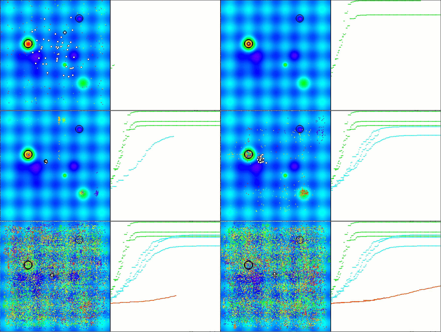
ANS on the Hilly test function
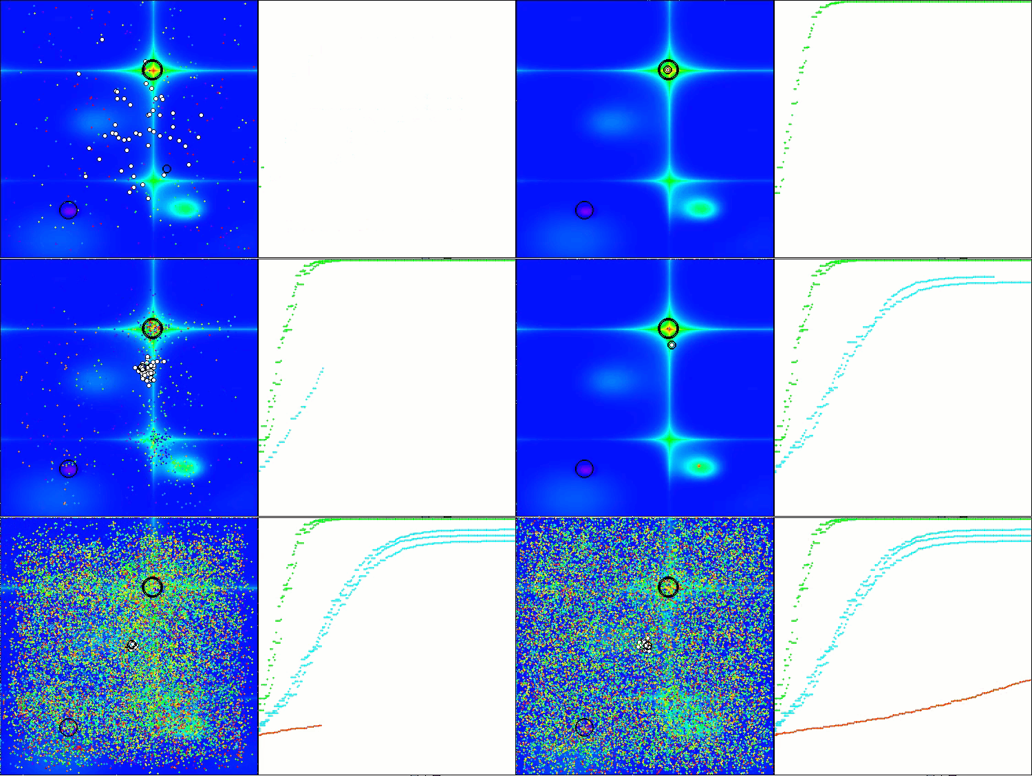
ANS on the Forest test function
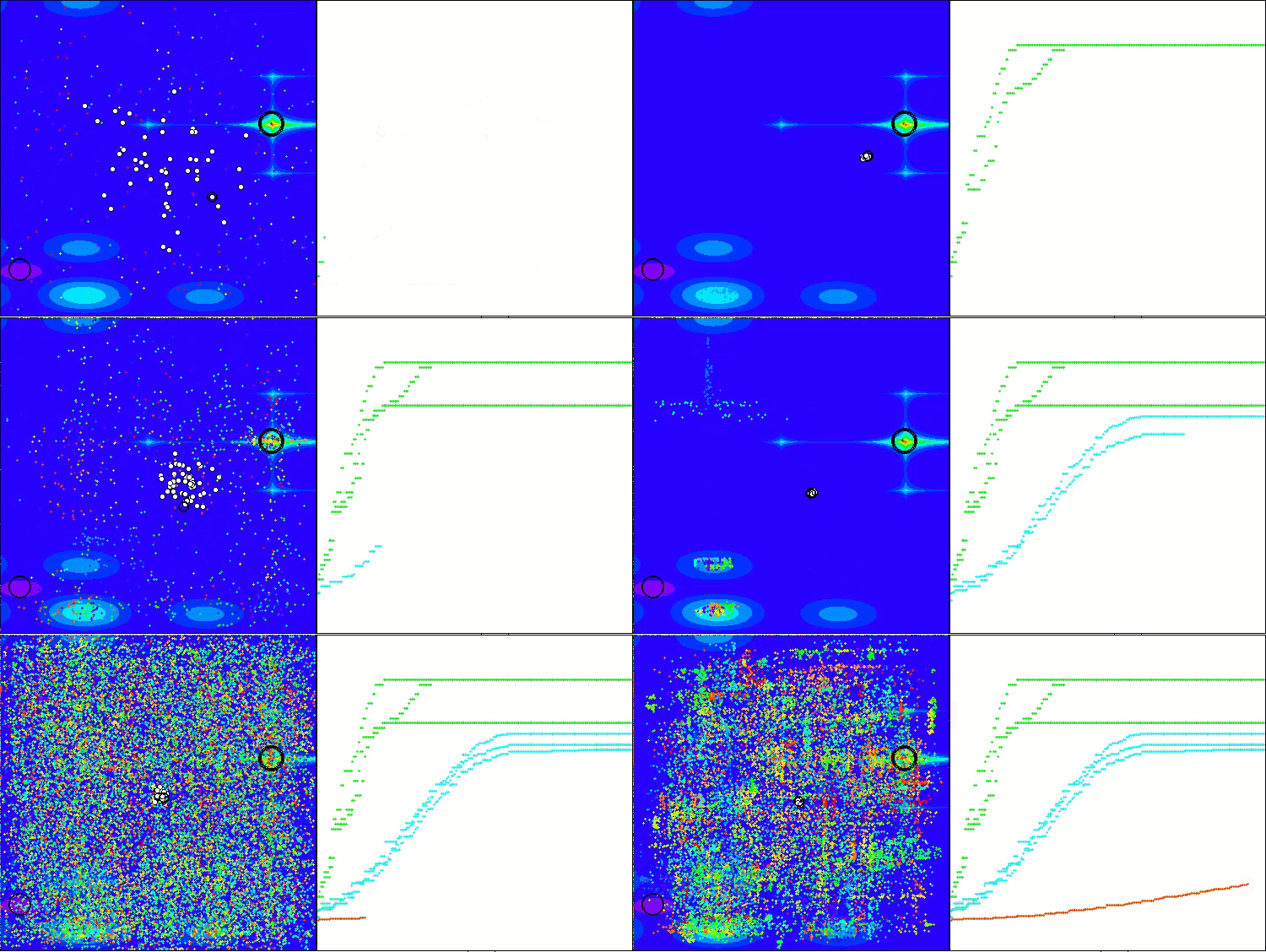
ANS on the Megacity test function
The algorithm considered in this article confidently took second place in the rating table. The algorithm demonstrates impressive scalability, maintaining the ability to search even on large-dimensional problems.
| # | AO | Description | Hilly | Hilly final | Forest | Forest final | Megacity (discrete) | Megacity final | Final result | % of MAX | ||||||
| 10 p (5 F) | 50 p (25 F) | 1000 p (500 F) | 10 p (5 F) | 50 p (25 F) | 1000 p (500 F) | 10 p (5 F) | 50 p (25 F) | 1000 p (500 F) | ||||||||
| 1 | BGA | binary genetic algorithm | 0.99989 | 0.99518 | 0.42835 | 2.42341 | 0.96153 | 0.96181 | 0.32027 | 2.24360 | 0.91385 | 0.95908 | 0.24220 | 2.11512 | 6.782 | 75.36 |
| 2 | ANS | across neighbourhood search | 0.94948 | 0.84776 | 0.43857 | 2.23581 | 1.00000 | 0.92334 | 0.39988 | 2.32323 | 0.70923 | 0.63477 | 0.23091 | 1.57491 | 6.134 | 68.15 |
| 3 | CLA | code lock algorithm | 0.95345 | 0.87107 | 0.37590 | 2.20042 | 0.98942 | 0.91709 | 0.31642 | 2.22294 | 0.79692 | 0.69385 | 0.19303 | 1.68380 | 6.107 | 67.86 |
| 4 | (P+O)ES | (P+O) evolution strategies | 0.92256 | 0.88101 | 0.40021 | 2.20379 | 0.97750 | 0.87490 | 0.31945 | 2.17185 | 0.67385 | 0.62985 | 0.18634 | 1.49003 | 5.866 | 65.17 |
| 5 | CTA | comet tail algorithm | 0.95346 | 0.86319 | 0.27770 | 2.09435 | 0.99794 | 0.85740 | 0.33949 | 2.19484 | 0.88769 | 0.56431 | 0.10512 | 1.55712 | 5.846 | 64.96 |
| 6 | SDSm | stochastic diffusion search M | 0.93066 | 0.85445 | 0.39476 | 2.17988 | 0.99983 | 0.89244 | 0.19619 | 2.08846 | 0.72333 | 0.61100 | 0.10670 | 1.44103 | 5.709 | 63.44 |
| 7 | ESG | evolution of social groups | 0.99906 | 0.79654 | 0.35056 | 2.14616 | 1.00000 | 0.82863 | 0.13102 | 1.95965 | 0.82333 | 0.55300 | 0.04725 | 1.42358 | 5.529 | 61.44 |
| 8 | SIA | simulated isotropic annealing | 0.95784 | 0.84264 | 0.41465 | 2.21513 | 0.98239 | 0.79586 | 0.20507 | 1.98332 | 0.68667 | 0.49300 | 0.09053 | 1.27020 | 5.469 | 60.76 |
| 9 | ACS | artificial cooperative search | 0.75547 | 0.74744 | 0.30407 | 1.80698 | 1.00000 | 0.88861 | 0.22413 | 2.11274 | 0.69077 | 0.48185 | 0.13322 | 1.30583 | 5.226 | 58.06 |
| 10 | TSEA | turtle shell evolution algorithm | 0.96798 | 0.64480 | 0.29672 | 1.90949 | 0.99449 | 0.61981 | 0.22708 | 1.84139 | 0.69077 | 0.42646 | 0.13598 | 1.25322 | 5.004 | 55.60 |
| 11 | DE | differential evolution | 0.95044 | 0.61674 | 0.30308 | 1.87026 | 0.95317 | 0.78896 | 0.16652 | 1.90865 | 0.78667 | 0.36033 | 0.02953 | 1.17653 | 4.955 | 55.06 |
| 12 | CRO | chemical reaction optimization | 0.94629 | 0.66112 | 0.29853 | 1.90593 | 0.87906 | 0.58422 | 0.21146 | 1.67473 | 0.75846 | 0.42646 | 0.12686 | 1.31178 | 4.892 | 54.36 |
| 13 | BSA | bird swarm algorithm | 0.89306 | 0.64900 | 0.26250 | 1.80455 | 0.92420 | 0.71121 | 0.24939 | 1.88479 | 0.69385 | 0.32615 | 0.10012 | 1.12012 | 4.809 | 53.44 |
| 14 | HS | harmony search | 0.86509 | 0.68782 | 0.32527 | 1.87818 | 0.99999 | 0.68002 | 0.09590 | 1.77592 | 0.62000 | 0.42267 | 0.05458 | 1.09725 | 4.751 | 52.79 |
| 15 | SSG | saplings sowing and growing | 0.77839 | 0.64925 | 0.39543 | 1.82308 | 0.85973 | 0.62467 | 0.17429 | 1.65869 | 0.64667 | 0.44133 | 0.10598 | 1.19398 | 4.676 | 51.95 |
| 16 | (PO)ES | (PO) evolution strategies | 0.79025 | 0.62647 | 0.42935 | 1.84606 | 0.87616 | 0.60943 | 0.19591 | 1.68151 | 0.59000 | 0.37933 | 0.11322 | 1.08255 | 4.610 | 51.22 |
| 17 | BSO | brain storm optimization | 0.93736 | 0.57616 | 0.29688 | 1.81041 | 0.93131 | 0.55866 | 0.23537 | 1.72534 | 0.55231 | 0.29077 | 0.11914 | 0.96222 | 4.498 | 49.98 |
| 18 | WOAm | wale optimization algorithm M | 0.84521 | 0.56298 | 0.26263 | 1.67081 | 0.93100 | 0.52278 | 0.16365 | 1.61743 | 0.66308 | 0.41138 | 0.11357 | 1.18803 | 4.476 | 49.74 |
| 19 | ACOm | ant colony optimization M | 0.88190 | 0.66127 | 0.30377 | 1.84693 | 0.85873 | 0.58680 | 0.15051 | 1.59604 | 0.59667 | 0.37333 | 0.02472 | 0.99472 | 4.438 | 49.31 |
| 20 | BFO-GA | bacterial foraging optimization - ga | 0.89150 | 0.55111 | 0.31529 | 1.75790 | 0.96982 | 0.39612 | 0.06305 | 1.42899 | 0.72667 | 0.27500 | 0.03525 | 1.03692 | 4.224 | 46.93 |
| 21 | MEC | mind evolutionary computation | 0.69533 | 0.53376 | 0.32661 | 1.55569 | 0.72464 | 0.33036 | 0.07198 | 1.12698 | 0.52500 | 0.22000 | 0.04198 | 0.78698 | 3.470 | 38.55 |
| 22 | IWO | invasive weed optimization | 0.72679 | 0.52256 | 0.33123 | 1.58058 | 0.70756 | 0.33955 | 0.07484 | 1.12196 | 0.42333 | 0.23067 | 0.04617 | 0.70017 | 3.403 | 37.81 |
| 23 | Micro-AIS | micro artificial immune system | 0.79547 | 0.51922 | 0.30861 | 1.62330 | 0.72956 | 0.36879 | 0.09398 | 1.19233 | 0.37667 | 0.15867 | 0.02802 | 0.56335 | 3.379 | 37.54 |
| 24 | COAm | cuckoo optimization algorithm M | 0.75820 | 0.48652 | 0.31369 | 1.55841 | 0.74054 | 0.28051 | 0.05599 | 1.07704 | 0.50500 | 0.17467 | 0.03380 | 0.71347 | 3.349 | 37.21 |
| 25 | SDOm | spiral dynamics optimization M | 0.74601 | 0.44623 | 0.29687 | 1.48912 | 0.70204 | 0.34678 | 0.10944 | 1.15826 | 0.42833 | 0.16767 | 0.03663 | 0.63263 | 3.280 | 36.44 |
| 26 | NMm | Nelder-Mead method M | 0.73807 | 0.50598 | 0.31342 | 1.55747 | 0.63674 | 0.28302 | 0.08221 | 1.00197 | 0.44667 | 0.18667 | 0.04028 | 0.67362 | 3.233 | 35.92 |
| 27 | FAm | firefly algorithm M | 0.58634 | 0.47228 | 0.32276 | 1.38138 | 0.68467 | 0.37439 | 0.10908 | 1.16814 | 0.28667 | 0.16467 | 0.04722 | 0.49855 | 3.048 | 33.87 |
| 28 | GSA | gravitational search algorithm | 0.64757 | 0.49197 | 0.30062 | 1.44016 | 0.53962 | 0.36353 | 0.09945 | 1.00260 | 0.32667 | 0.12200 | 0.01917 | 0.46783 | 2.911 | 32.34 |
| 29 | BFO | bacterial foraging optimization | 0.61171 | 0.43270 | 0.31318 | 1.35759 | 0.54410 | 0.21511 | 0.05676 | 0.81597 | 0.42167 | 0.13800 | 0.03195 | 0.59162 | 2.765 | 30.72 |
| 30 | ABC | artificial bee colony | 0.63377 | 0.42402 | 0.30892 | 1.36671 | 0.55103 | 0.21874 | 0.05623 | 0.82600 | 0.34000 | 0.14200 | 0.03102 | 0.51302 | 2.706 | 30.06 |
| 31 | BA | bat algorithm | 0.59761 | 0.45911 | 0.35242 | 1.40915 | 0.40321 | 0.19313 | 0.07175 | 0.66810 | 0.21000 | 0.10100 | 0.03517 | 0.34617 | 2.423 | 26.93 |
| 32 | SA | simulated annealing | 0.55787 | 0.42177 | 0.31549 | 1.29513 | 0.34998 | 0.15259 | 0.05023 | 0.55280 | 0.31167 | 0.10033 | 0.02883 | 0.44083 | 2.289 | 25.43 |
| 33 | IWDm | intelligent water drops M | 0.54501 | 0.37897 | 0.30124 | 1.22522 | 0.46104 | 0.14704 | 0.04369 | 0.65177 | 0.25833 | 0.09700 | 0.02308 | 0.37842 | 2.255 | 25.06 |
| 34 | PSO | particle swarm optimisation | 0.59726 | 0.36923 | 0.29928 | 1.26577 | 0.37237 | 0.16324 | 0.07010 | 0.60572 | 0.25667 | 0.08000 | 0.02157 | 0.35823 | 2.230 | 24.77 |
| 35 | Boids | boids algorithm | 0.43340 | 0.30581 | 0.25425 | 0.99346 | 0.35718 | 0.20160 | 0.15708 | 0.71586 | 0.27846 | 0.14277 | 0.09834 | 0.51957 | 2.229 | 24.77 |
| 36 | MA | monkey algorithm | 0.59107 | 0.42681 | 0.31816 | 1.33604 | 0.31138 | 0.14069 | 0.06612 | 0.51819 | 0.22833 | 0.08567 | 0.02790 | 0.34190 | 2.196 | 24.40 |
| 37 | SFL | shuffled frog-leaping | 0.53925 | 0.35816 | 0.29809 | 1.19551 | 0.37141 | 0.11427 | 0.04051 | 0.52618 | 0.27167 | 0.08667 | 0.02402 | 0.38235 | 2.104 | 23.38 |
| 38 | FSS | fish school search | 0.55669 | 0.39992 | 0.31172 | 1.26833 | 0.31009 | 0.11889 | 0.04569 | 0.47467 | 0.21167 | 0.07633 | 0.02488 | 0.31288 | 2.056 | 22.84 |
| 39 | RND | random | 0.52033 | 0.36068 | 0.30133 | 1.18234 | 0.31335 | 0.11787 | 0.04354 | 0.47476 | 0.25333 | 0.07933 | 0.02382 | 0.35648 | 2.014 | 22.37 |
| 40 | GWO | grey wolf optimizer | 0.59169 | 0.36561 | 0.29595 | 1.25326 | 0.24499 | 0.09047 | 0.03612 | 0.37158 | 0.27667 | 0.08567 | 0.02170 | 0.38403 | 2.009 | 22.32 |
| 41 | CSS | charged system search | 0.44252 | 0.35454 | 0.35201 | 1.14907 | 0.24140 | 0.11345 | 0.06814 | 0.42299 | 0.18333 | 0.06300 | 0.02322 | 0.26955 | 1.842 | 20.46 |
| 42 | EM | electroMagnetism-like algorithm | 0.46250 | 0.34594 | 0.32285 | 1.13129 | 0.21245 | 0.09783 | 0.10057 | 0.41085 | 0.15667 | 0.06033 | 0.02712 | 0.24412 | 1.786 | 19.85 |
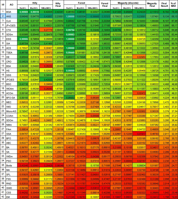
Figure 1. Color gradation of algorithms according to relevant tests Results greater than or equal to 0.99 are highlighted in white
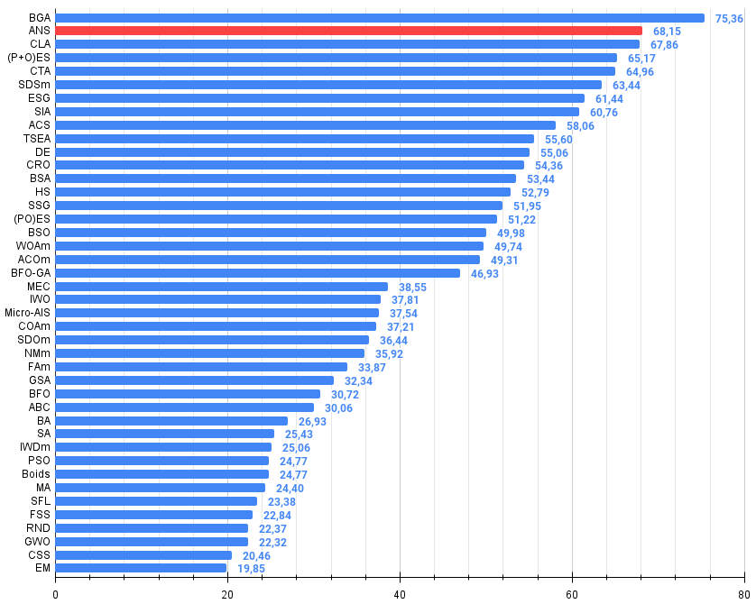
Figure 2. The histogram of algorithm test results (on a scale from 0 to 100, the more the better,
where 100 is the maximum possible theoretical result, the archive features a script for calculating the rating table)
Earlier in the article, we noted the tendency of the ANS algorithm population to degenerate. To address this major drawback, I decided to modify the algorithm by adding a mutation operator. In this case, the mutation will be a Gaussian probability of obtaining a new coordinate in the vicinity of the agent's best solution, but in the range from the minimum to the maximum acceptable value for the corresponding coordinate. To do this, we will need to make some changes to the Moving method.
Let's look at what changes were made to the code and briefly describe the method logic:
- If the random number is less than 0.005, a mutation occurs using a normal distribution.
- Otherwise, a random solution is selected from the collection, or the best agent coordinates are used.
- The distance and range for a normal distribution are calculated.
- Normal distribution is used to obtain new coordinate values.
//----------------------------------------------------------------------------
double min  = 0.0;
double max  = 0.0;
double dist = 0.0;
int    ind  = 0;
double r    = 0.0;
double p    = 0.0;

for (int i = 0; i < popSize; i++)
{
  for (int c = 0; c < coords; c++)
  {
    if (u.RNDprobab () < 0.005)
    {
      val = u.GaussDistribution (agent [i].cBest [c], rangeMin [c], rangeMax [c], sigma);
      val = u.SeInDiSp (val, rangeMin [c], rangeMax [c], rangeStep [c]);
    }
    else
    {
      if (u.RNDprobab () < collChoiceProbab)
      {
        do ind = u.RNDminusOne (collectionSize);
        while (coll [ind].f == -DBL_MAX);

        p = agent [i].c   [c];
        r = coll  [ind].c [c];

      }
      else
      {
        p = agent [i].c     [c];
        r = agent [i].cBest [c];
      }

      dist = fabs (p - r) * range;
      min  = r - dist;
      max  = r + dist;

      if (min < rangeMin [c]) min = rangeMin [c];
      if (max > rangeMax [c]) max = rangeMax [c];

      val = u.GaussDistribution (r, min, max, sigma);
      val = u.SeInDiSp (val, rangeMin [c], rangeMax [c], rangeStep [c]);
    }

    agent [i].c [c] = val;
    a     [i].c [c] = val;
  }
}
After adding the mutation operator, the algorithm continues to explore the search space for any number of epochs, as demonstrated in Figure 3 (a screenshot of the algorithm visualization).
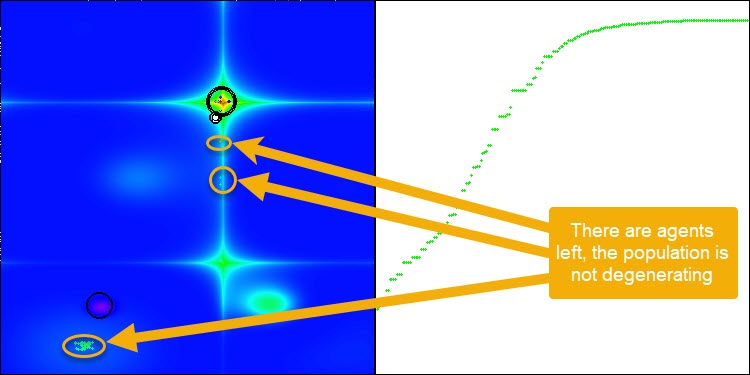
Figure 3. Agents have been left, population does not degenerate (parameter mut = 0.005)
- The mutation operator with mut 0.1 has a negative impact on the overall result. With such a large mutation ratio (10% of the total number of operations on each coordinate), we observe a deterioration in the algorithm performance. Therefore, I decided to gradually reduce this parameter. Decreasing the parameter value improved the results, and I settled on the value of 0.005. This ratio turned out to be sufficient to prevent population degeneration while still providing improved algorithm performance, as shown below.
Results of the algorithm operation with mutation probability mut = 0.1:
=============================
All score: 6.05103 (67.23%)
ANS|Across Neighbourhood Search|50.0|100.0|8.0|1.0|0.6|
=============================
5 Hilly's; Func runs: 10000; result: 0.9534829314854332
25 Hilly's; Func runs: 10000; result: 0.8136803288623282
500 Hilly's; Func runs: 10000; result: 0.31144979106165716
=============================
5 Forest's; Func runs: 10000; result: 0.9996561274415626
25 Forest's; Func runs: 10000; result: 0.81670393859872
500 Forest's; Func runs: 10000; result: 0.25620559379918284
=============================
5 Megacity's; Func runs: 10000; result: 0.8753846153846153
25 Megacity's; Func runs: 10000; result: 0.5778461538461539
500 Megacity's; Func runs: 10000; result: 0.13375384615384744
=============================
All score: 5.73816 (63.76%)
Results of the algorithm operation with mutation probability mut = 0.01:
=============================
5 Hilly's; Func runs: 10000; result: 0.9073657389037575
25 Hilly's; Func runs: 10000; result: 0.871278233418226
500 Hilly's; Func runs: 10000; result: 0.3960769225373809
=============================
5 Forest's; Func runs: 10000; result: 0.989394440004635
25 Forest's; Func runs: 10000; result: 0.9513150500729907
500 Forest's; Func runs: 10000; result: 0.35407610928209116
=============================
5 Megacity's; Func runs: 10000; result: 0.7492307692307691
25 Megacity's; Func runs: 10000; result: 0.6387692307692309
500 Megacity's; Func runs: 10000; result: 0.19352307692307838
=============================
All score: 6.05103 (67.23%)
Results of the algorithm operation with mutation probability mut = 0.005:
ANS|Across Neighbourhood Search|50.0|100.0|8.0|1.0|0.6|
=============================
5 Hilly's; Func runs: 10000; result: 0.949632264944664
25 Hilly's; Func runs: 10000; result: 0.871206955779846
500 Hilly's; Func runs: 10000; result: 0.40738389742274217
=============================
5 Forest's; Func runs: 10000; result: 0.9924803131691761
25 Forest's; Func runs: 10000; result: 0.9493489251290264
500 Forest's; Func runs: 10000; result: 0.3666276564633121
=============================
5 Megacity's; Func runs: 10000; result: 0.8061538461538461
25 Megacity's; Func runs: 10000; result: 0.6732307692307691
500 Megacity's; Func runs: 10000; result: 0.20844615384615534
=============================
All score: 6.22451 (69.16%)
Summary
Now that we have looked at the results of working together with the mutation operator, we can draw the following conclusions:
1. Simplicity and ease of implementation.
2. Balance between exploration and exploitation.
3. Efficiency in solving various types of problems.
4. Adaptability to various tasks.
5. Potential for further improvement.
Thus, ANS is a simple yet effective optimization algorithm that demonstrates competitive results on a wide range of problems and has potential for further development.
ANS general pros and cons:
Advantages:
- Good convergence on various types of functions.
- Very fast EA.
- Simple implementation.
- Excellent scalability.
Disadvantages:
- Sometimes gets stuck in local extremes.
The article is accompanied by an archive with the current versions of the algorithm codes. The author of the article is not responsible for the absolute accuracy in the description of canonical algorithms. Changes have been made to many of them to improve search capabilities. The conclusions and judgments presented in the articles are based on the results of the experiments.
Translated from Russian by MetaQuotes Ltd.
Original article: https://www.mql5.com/ru/articles/15049
Warning: All rights to these materials are reserved by MetaQuotes Ltd. Copying or reprinting of these materials in whole or in part is prohibited.
This article was written by a user of the site and reflects their personal views. MetaQuotes Ltd is not responsible for the accuracy of the information presented, nor for any consequences resulting from the use of the solutions, strategies or recommendations described.
 Build Self Optimizing Expert Advisors in MQL5 (Part 2): USDJPY Scalping Strategy
 Building a Candlestick Trend Constraint Model (Part 9): Multiple Strategies Expert Advisor (III)
 Automating Trading Strategies in MQL5 (Part 2): The Kumo Breakout System with Ichimoku and Awesome Oscillator
 Price Action Analysis Toolkit Development (Part 5): Volatility Navigator EA
- Free trading apps
- Over 8,000 signals for copying
- Economic news for exploring financial markets
You agree to website policy and terms of use