Creating a mean-reversion strategy based on machine learning

Introduction

This article proposes another original approach to creating trading systems based on machine learning. In the previous article, I have already considered the ways of applying clustering to the problem of causal inference. In this article, clustering will be used to divide financial time series into several modes with unique properties, and then trading systems will be built and tested on each of them.

In addition, we will look at several ways to label examples for mean reversion strategies and test them on the EURGBP currency pair, which is considered to be flat, meaning these strategies should be fully applicable to it.

This article will allow you to train various machine learning models in Python and convert them into trading systems for the MetaTrader 5 trading terminal.

Preparing the necessary packages

Model training will be done in Python, so please make sure you have the following packages installed:

import math
import pandas as pd
import pickle
from datetime import datetime
from catboost import CatBoostClassifier

from sklearn.model_selection import train_test_split
from sklearn.cluster import KMeans

from bots.botlibs.labeling_lib import *
from bots.botlibs.tester_lib import tester
from bots.botlibs.export_lib import export_model_to_ONNX

The last 3 modules were written by me. They are attached at the end of the article. Each of them may import other packages, such as Scipy, Numpy, Sklearn, Numba, which should also be installed. They are widely known and publicly available, so there should be no problems installing them.

If you have a clean version of Python, below is a list of packages you will need to install:

pip install numpy
pip install pandas
pip install scipy
pip install scikit-learn
pip install catboost
pip install numba

You may also need to use absolute import paths for the libraries included at the end of the article, depending on your development environment and their location.

The code is designed in such a way that it does not depend heavily on the version of the Python interpreter or a specific package, but it is better to use the latest stable versions.

How can examples for mean reversion strategies be labeled?

Let's recall how we marked up the labels in previous articles. We created a loop, in which the duration of each individual trade was randomly set, for example, from 1 to 15 bars. Then, depending on whether the market had risen or fallen within the number of bars that had passed since the virtual trade was opened, a buy or sell mark was placed. The function returned a dataframe with features and labeled tags, and the dataset was already fully prepared for subsequent training of a machine learning model on it.

def get_labels(dataset, markup, min = 1, max = 15) -> pd.DataFrame:
    labels = []
    for i in range(dataset.shape[0]-max):
        rand = random.randint(min, max)
        curr_pr = dataset['close'].iloc[i]
        future_pr = dataset['close'].iloc[i + rand]

        if (future_pr + markup) < curr_pr:
            labels.append(1.0)
        elif (future_pr - markup) > curr_pr:
            labels.append(0.0)
        else:
            labels.append(2.0)
        
    dataset = dataset.iloc[:len(labels)].copy()
    dataset['labels'] = labels
    dataset = dataset.dropna()
    dataset = dataset.drop(
        dataset[dataset.labels == 2.0].index)
    return dataset

But this type of labeling has one significant drawback - it is random. By labeling the data this way, we do not impose any idea about what patterns the machine learning model should approximate. Therefore, the result of such labeling and training will also be, to a large extent, random. We tried to fix this by running multiple brute-force training runs and making the algorithm architectures more complex, but the labeling itself was still meaningless. Due to random sampling, only some models could pass OOS (out-of-sample test).

In this article, I propose a new approach for trade labeling based on filtering the original time series. Let's take a look at this labeling using an example.

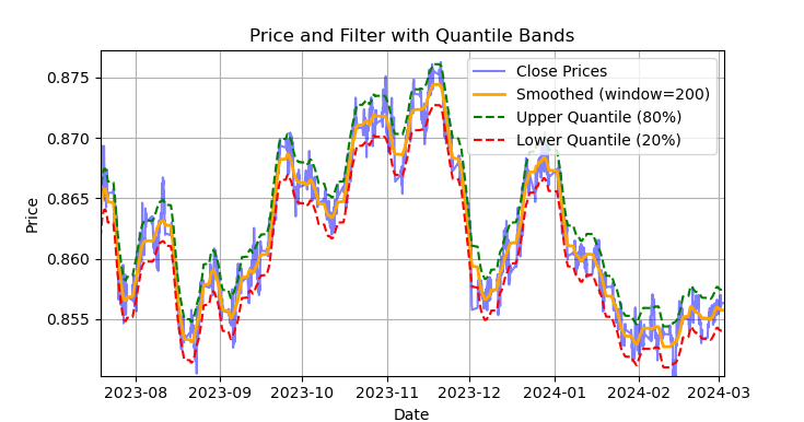
Fig. 1. Display of the Savitzky-Golay filter and bands (quantiles)

Fig. 1 shows the smoothing line of the Savitzky-Golay filter and the 20 and 80 quantile bands, somewhat reminiscent of Bollinger Bands. The main difference between the Savitzky-Golay filter and a regular moving average is that it does not lag relative to prices. Due to this property, the filter smooths prices well, and the residual "noise" is deviations from the mean values (the values of the filter itself), which can be used to develop a mean reversion strategy. When the upper and lower bands cross, a sell or buy signal is formed. If the price crosses the upper line, it is a sell signal. If the price crosses the lower line, this is a buy signal.

The Savitzky-Golay filter is a digital filter used to smooth data and suppress noise while preserving important signal features such as peaks and trends. It was proposed by Abraham Savitzky and Marcel J. Е. Golay in 1964. This filter is widely used in signal processing and data analysis.

The Savitzky-Golay filter operates by locally approximating the data with a low-degree (quadratic, cubic or quartic) polynomial using the least-squares method. For each data point, a neighborhood (window) is selected, and the data within this window is approximated by the polynomial. After approximation, the value at the center of the window is replaced by the value calculated using the polynomial. This allows us to smooth out noise while maintaining the signal form.

Below is the code for constructing and visually evaluating the filter.

def plot_close_filter_quantiles(dataset, rolling=200, quantiles=[0.2, 0.8], polyorder=3):
    # Calculate smoothed prices
    smoothed = savgol_filter(dataset['close'], 
                            window_length=rolling, 
                            polyorder=polyorder)
    
    # Calculate difference between prices and filter
    lvl = dataset['close'] - smoothed
    
    # Get quantile values
    q_low, q_high = lvl.quantile(quantiles).tolist()
    
    # Calculate bands based on quantiles
    upper_band = smoothed + q_high  # Upper band
    lower_band = smoothed + q_low   # Lower band
    
    # Create plot
    plt.figure(figsize=(14, 7))
    plt.plot(dataset.index, dataset['close'], label='Close Prices', color='blue', alpha=0.5)
    plt.plot(dataset.index, smoothed, label=f'Smoothed (window={rolling})', color='orange', linewidth=2)
    plt.plot(dataset.index, upper_band, label=f'Upper Quantile ({quantiles[1]*100:.0f}%)', 
             color='green', linestyle='--')
    plt.plot(dataset.index, lower_band, label=f'Lower Quantile ({quantiles[0]*100:.0f}%)', 
             color='red', linestyle='--')
    
    # Configure display
    plt.title('Price and Filter with Quantile Bands')
    plt.xlabel('Date')
    plt.ylabel('Price')
    plt.legend()
    plt.grid(True)
    plt.show()

Thus, it would be a mistake to use this filter online on non-stationary time series, since the latest values may be redrawn, but it is quite suitable for marking trades on existing data.

Let's write the code that will implement labeling of training examples using the Savitzky-Golay filter. The labeling function, along with other similar functions, is located in the labeling_lib.py Python module, which will then be imported into our project.

@njit
def calculate_labels_filter(close, lvl, q):
    labels = np.empty(len(close), dtype=np.float64)
    for i in range(len(close)):
        curr_lvl = lvl[i]

        if curr_lvl > q[1]:
            labels[i] = 1.0
        elif curr_lvl < q[0]:
            labels[i] = 0.0
        else:
            labels[i] = 2.0
    return labels

def get_labels_filter(dataset, rolling=200, quantiles=[.45, .55], polyorder=3) -> pd.DataFrame:
    """
    Generates labels for a financial dataset based on price deviation from a Savitzky-Golay filter.

    This function applies a Savitzky-Golay filter to the closing prices to generate a smoothed
    price trend. It then calculates trading signals (buy/sell) based on the deviation of the 
    actual price from this smoothed trend. Buy signals are generated when the price is 
    significantly below the smoothed trend, anticipating a potential price reversal. 

    Args:
        dataset (pd.DataFrame): DataFrame containing financial data with a 'close' column.
        rolling (int, optional): Window size for the Savitzky-Golay filter. Defaults to 200.
        quantiles (list, optional): Quantiles to define the "reversion zone". Defaults to [.45, .55].
        polyorder (int, optional): Polynomial order for the Savitzky-Golay filter. Defaults to 3.

    Returns:
        pd.DataFrame: The original DataFrame with a new 'labels' column and filtered rows:
                       - 'labels' column: 
                            - 0: Buy
                            - 1: Sell
                       - Rows where 'labels' is 2 (no signal) are removed.
                       - Rows with missing values (NaN) are removed.
                       - The temporary 'lvl' column is removed. 
    """

    # Calculate smoothed prices using the Savitzky-Golay filter
    smoothed_prices = savgol_filter(dataset['close'].values, window_length=rolling, polyorder=polyorder)
    
    # Calculate the difference between the actual closing prices and the smoothed prices
    diff = dataset['close'] - smoothed_prices
    dataset['lvl'] = diff  # Add the difference as a new column 'lvl' to the DataFrame
    
    # Remove any rows with NaN values 
    dataset = dataset.dropna()
    
    # Calculate the quantiles of the 'lvl' column (price deviation)
    q = dataset['lvl'].quantile(quantiles).to_list() 

    # Extract the closing prices and the calculated 'lvl' values as NumPy arrays
    close = dataset['close'].values
    lvl = dataset['lvl'].values
    
    # Calculate buy/sell labels using the 'calculate_labels_filter' function 
    labels = calculate_labels_filter(close, lvl, q) 

    # Trim the dataset to match the length of the calculated labels
    dataset = dataset.iloc[:len(labels)].copy()
    
    # Add the calculated labels as a new 'labels' column to the DataFrame
    dataset['labels'] = labels
    
    # Remove any rows with NaN values
    dataset = dataset.dropna()
    
    # Remove rows where the 'labels' column has a value of 2.0 (no signals)
    dataset = dataset.drop(dataset[dataset.labels == 2.0].index)
    
    # Return the modified DataFrame with the 'lvl' column removed
    return dataset.drop(columns=['lvl']) 

To speed up labeling, we use the Numba package described in the previous article.

The get_labels_filter() function accepts the original dataset with prices and features constructed from them, the length of the approximation window for the filter, the boundaries of the lower and upper quantiles, and the degree of the polynomial. The output of this function is to add buy or sell labels to the original dataset, which can then be used as a training dataset.

The history loop is implemented in a separate function named calc_labels_filter, which performs heavy calculations using the Numba package.

This type of labeling has its own characteristics:

• not all marked trades are profitable, since further price changes after crossing the bands do not always go in the opposite direction. This may result in examples being falsely labeled as buy or sell.
• this drawback is, in theory, compensated by the fact that labeling is uniform and non-random, and therefore falsely labeled examples can be considered as training errors or errors of the trading system as a whole, which can result in less overfitting at the output.

The full description of the deal labeling logic is presented below:

calculate_labels_filter function

Input data:

• close - array of close prices
• lvl - array of price deviations from the smoothed trend
• q - array of quantiles defining signal zones

Logic:

1. Initialization: Create an empty 'labels' array of the same length as 'close' to store the signals.

2. Loop through prices: For each close[i] price and corresponding lvl[i] deviation:

• Sell signal: If the lvl[i] deviation exceeds the upper quantile q[1], the price is located significantly above the smoothed trend, which indicates the Sell signal (labels[i] = 1.0).
• Buy signal: If the lvl[i] deviation is less than the lower quantile q[0], the price is significantly below the smoothed trend, which indicates the Buy signal (labels[i] = 0.0).
• No signal: In other cases (deviation is between quantiles), no signal is generated (labels[i] = 2.0).

3. Return result: Return the 'labels' array with signals.

get_labels_filter function

Input data:

• dataset - DataFrame with financial data containing the 'close' column (close prices)
• rolling - window size for smoothing the Savitzky-Golay filter
• quantiles - quantiles for determining signal zones
• polyorder - order of the polynomial for Savitzky-Golay smoothing

Logic:

1. Price smoothing:

• Calculate smoothed_prices using the Savitzky-Golay filter applied to close prices (dataset['close']).

2. Calculating the deviation:

• We calculate the difference (diff) between the actual close prices and the smoothed prices.
• We also add the difference as a new 'lvl' column to the DataFrame.

3. Removing gaps:

• Remove rows with missing values (NaN) from DataFrame.

4. Calculating quantiles:

• Calculate quantiles for the 'lvl' column, which will be used to determine signal zones.

5. Signal calculation:

• Call the calculate_labels_filter function, passing it the closing prices, deviations, and quantiles. 
• Get the 'labels' array with signals.

6. DataFrame handling:

• Truncate the DataFrame to the length of the 'labels' array.
• Add the 'labels' array as a new 'labels' column to DataFrame.
• Remove strings where 'labels' is equal to 2.0 (no signal).
• Remove the temporary 'lvl' column.

7. Return result: Return a modified DataFrame with the Buy and Sell signals in the 'labels' column.

We will consider the above labeling method as a standard, by means of which the basic principles of the mean reversion strategy markup are demonstrated. This is a working method that can be used. We can generalize and modify it to accommodate multiple filters and to account for variable variance in deviations from the mean. Below is the get_labels_multiple_filters function that implements such changes.

@njit
def calc_labels_multiple_filters(close, lvls, qs):
    labels = np.empty(len(close), dtype=np.float64)
    for i in range(len(close)):
        label_found = False
        
        for j in range(len(lvls)):
            curr_lvl = lvls[j][i]
            curr_q_low = qs[j][0][i]
            curr_q_high = qs[j][1][i]
            
            if curr_lvl > curr_q_high:
                labels[i] = 1.0
                label_found = True
                break
            elif curr_lvl < curr_q_low:
                labels[i] = 0.0
                label_found = True
                break
                
        if not label_found:
            labels[i] = 2.0
            
    return labels

def get_labels_multiple_filters(dataset, 
                              rolling_periods=[200, 400, 600], 
                              quantiles=[.45, .55], 
                              window=100,
                              polyorder=3) -> pd.DataFrame:
    """
    Generates trading signals (buy/sell) based on price deviation from multiple 
    smoothed price trends calculated using a Savitzky-Golay filter with different
    rolling periods and rolling quantiles. 

    This function applies a Savitzky-Golay filter to the closing prices for each 
    specified 'rolling_period'. It then calculates the price deviation from these
    smoothed trends and determines dynamic "reversion zones" using rolling quantiles.
    Buy signals are generated when the price is within these reversion zones 
    across multiple timeframes.

    Args:
        dataset (pd.DataFrame): DataFrame containing financial data with a 'close' column.
        rolling_periods (list, optional): List of rolling window sizes for the Savitzky-Golay filter. 
                                           Defaults to [200, 400, 600].
        quantiles (list, optional): Quantiles to define the "reversion zone". Defaults to [.05, .95].
        window (int, optional): Window size for calculating rolling quantiles. Defaults to 100.
        polyorder (int, optional): Polynomial order for the Savitzky-Golay filter. Defaults to 3.

    Returns:
        pd.DataFrame: The original DataFrame with a new 'labels' column and filtered rows:
                       - 'labels' column: 
                            - 0: Buy
                            - 1: Sell
                       - Rows where 'labels' is 2 (no signal) are removed.
                       - Rows with missing values (NaN) are removed. 
    """
    
    # Create a copy of the dataset to avoid modifying the original
    dataset = dataset.copy()
    
    # Lists to store price deviation levels and quantiles for each rolling period
    all_levels = []
    all_quantiles = []
    
    # Calculate smoothed price trends and rolling quantiles for each rolling period
    for rolling in rolling_periods:
        # Calculate smoothed prices using the Savitzky-Golay filter
        smoothed_prices = savgol_filter(dataset['close'].values, 
                                      window_length=rolling, 
                                      polyorder=polyorder)
        # Calculate the price deviation from the smoothed prices
        diff = dataset['close'] - smoothed_prices
        
        # Create a temporary DataFrame to calculate rolling quantiles
        temp_df = pd.DataFrame({'diff': diff})
        
        # Calculate rolling quantiles for the price deviation
        q_low = temp_df['diff'].rolling(window=window).quantile(quantiles[0])
        q_high = temp_df['diff'].rolling(window=window).quantile(quantiles[1])
        
        # Store the price deviation and quantiles for the current rolling period
        all_levels.append(diff)
        all_quantiles.append([q_low.values, q_high.values])
    
    # Convert lists to NumPy arrays for faster calculations (potentially using Numba)
    lvls_array = np.array(all_levels)
    qs_array = np.array(all_quantiles)
    
    # Calculate buy/sell labels using the 'calc_labels_multiple_filters' function 
    labels = calc_labels_multiple_filters(dataset['close'].values, lvls_array, qs_array)
    
    # Add the calculated labels to the DataFrame
    dataset['labels'] = labels
    
    # Remove rows with NaN values and no signals (labels == 2.0)
    dataset = dataset.dropna()
    dataset = dataset.drop(dataset[dataset.labels == 2.0].index)
    
    # Return the DataFrame with the new 'labels' column
    return dataset

This function can accept an unlimited number of smoothing parameters for the Savitzky-Golay filter. This can provide an additional benefit since labeling will involve multiple filters with different periods. To form a signal, it is sufficient that deviations from the mean, at a distance of the quantile boundaries, are triggered for at least one of the filters.

This will allow us to build a hierarchical structure for marking deals. For example, the condition for the high-pass filter is checked first, then for the mid-pass filter, and then for the low-pass one. Low-pass filter signals can be considered more reliable, so previous signals will be overwritten by a low-pass filter signal if one occurs. But if the low-pass filter does not generate a signal, then the trades will still be marked based on the signals from the previous filters. This helps increase the number of labeled examples and allows for higher input thresholds (quantiles), because it increases the chance of at least one signal appearing across a set of filters.

Quantile calculations are now performed in a sliding window with a configurable period, which allows for variable variance of deviations from the mean to be taken into account for more accurate signals.

Finally, we can consider the case for asymmetric trades, assuming that filters with different smoothing periods may be required to mark buy and sell orders due to the skewed average of quotes. This approach is implemented in the get_labels_filter_bidirectional function.

@njit
def calc_labels_bidirectional(close, lvl1, lvl2, q1, q2):
    labels = np.empty(len(close), dtype=np.float64)
    for i in range(len(close)):
        curr_lvl1 = lvl1[i]
        curr_lvl2 = lvl2[i]

        if curr_lvl1 > q1[1]:
            labels[i] = 1.0
        elif curr_lvl2 < q2[0]:
            labels[i] = 0.0
        else:
            labels[i] = 2.0
    return labels

def get_labels_filter_bidirectional(dataset, rolling1=200, rolling2=200, quantiles=[.45, .55], polyorder=3) -> pd.DataFrame:
    """
    Generates trading labels based on price deviation from two Savitzky-Golay filters applied
    in opposite directions (forward and reversed) to the closing price data.

    This function calculates trading signals (buy/sell) based on the price's 
    position relative to smoothed price trends generated by two Savitzky-Golay filters 
    with potentially different window sizes (`rolling1`, `rolling2`). 

    Args:
        dataset (pd.DataFrame): DataFrame containing financial data with a 'close' column.
        rolling1 (int, optional): Window size for the first Savitzky-Golay filter. Defaults to 200.
        rolling2 (int, optional): Window size for the second Savitzky-Golay filter. Defaults to 200.
        quantiles (list, optional): Quantiles to define the "reversion zones". Defaults to [.45, .55].
        polyorder (int, optional): Polynomial order for both Savitzky-Golay filters. Defaults to 3.

    Returns:
        pd.DataFrame: The original DataFrame with a new 'labels' column and filtered rows:
                       - 'labels' column: 
                            - 0: Buy
                            - 1: Sell
                       - Rows where 'labels' is 2 (no signal) are removed.
                       - Rows with missing values (NaN) are removed.
                       - Temporary 'lvl1' and 'lvl2' columns are removed.
    """

    # Apply the first Savitzky-Golay filter (forward direction)
    smoothed_prices = savgol_filter(dataset['close'].values, window_length=rolling1, polyorder=polyorder)
    
    # Apply the second Savitzky-Golay filter (could be in reverse direction if rolling2 is negative)
    smoothed_prices2 = savgol_filter(dataset['close'].values, window_length=rolling2, polyorder=polyorder)

    # Calculate price deviations from both smoothed price series
    diff1 = dataset['close'] - smoothed_prices
    diff2 = dataset['close'] - smoothed_prices2

    # Add price deviations as new columns to the DataFrame
    dataset['lvl1'] = diff1
    dataset['lvl2'] = diff2
    
    # Remove rows with NaN values 
    dataset = dataset.dropna()

    # Calculate quantiles for the "reversion zones" for both price deviation series
    q1 = dataset['lvl1'].quantile(quantiles).to_list()
    q2 = dataset['lvl2'].quantile(quantiles).to_list()

    # Extract relevant data for label calculation
    close = dataset['close'].values
    lvl1 = dataset['lvl1'].values
    lvl2 = dataset['lvl2'].values
    
    # Calculate buy/sell labels using the 'calc_labels_bidirectional' function
    labels = calc_labels_bidirectional(close, lvl1, lvl2, q1, q2)

    # Process the dataset and labels
    dataset = dataset.iloc[:len(labels)].copy()
    dataset['labels'] = labels
    dataset = dataset.dropna()
    dataset = dataset.drop(dataset[dataset.labels == 2.0].index) # Remove bad signals (if any)
    
    # Return the DataFrame with temporary columns removed
    return dataset.drop(columns=['lvl1', 'lvl2']) 

This function accepts rolling1 and rolling2 smoothing periods, which correspond to sell and buy trades. By varying these parameters, one can attempt to achieve better labeling and generalization ability on new data. For example, if a currency pair is trending upward and it is more preferable to open buy trades, then you can increase the length of the roling1 window for marking sell trades, and there will be fewer of them, or they will only occur at the moments of really strong trend reversals. For buy trades, we can reduce the roling2 window length, so there will be more buy trades than sell ones.

Labeling with a restriction on profitable trades and filter selection

It was mentioned above that the proposed trade markers allow for the presence of marked but obviously unprofitable trades. This is not a bug, but rather a feature.

We can add checks to ensure that only profitable trades are marked. This can be useful if there is a need to bring the balance graph closer to an ideal straight line with no significant drawdowns.

Also, only a single Savitzky-Golay filter was used, but I would like to increase their diversity by adding a simple moving average and a spline as filters.

Let's look at the options for such trade samplers. We will use the get_labels_mean_reversion function as a basis, which provides for restrictions on profitability and filter selection.

@njit
def calculate_labels_mean_reversion(close, lvl, markup, min_l, max_l, q):
    labels = np.empty(len(close) - max_l, dtype=np.float64)
    for i in range(len(close) - max_l):
        rand = random.randint(min_l, max_l)
        curr_pr = close[i]
        curr_lvl = lvl[i]
        future_pr = close[i + rand]

        if curr_lvl > q[1] and (future_pr + markup) < curr_pr:
            labels[i] = 1.0
        elif curr_lvl < q[0] and (future_pr - markup) > curr_pr:
            labels[i] = 0.0
        else:
            labels[i] = 2.0
    return labels

def get_labels_mean_reversion(dataset, markup, min_l=1, max_l=15, rolling=0.5, quantiles=[.45, .55], method='spline', shift=0) -> pd.DataFrame:
    """
    Generates labels for a financial dataset based on mean reversion principles.

    This function calculates trading signals (buy/sell) based on the deviation of
    the price from a chosen moving average or smoothing method. It identifies
    potential buy opportunities when the price deviates significantly below its 
    smoothed trend, anticipating a reversion to the mean.

    Args:
        dataset (pd.DataFrame): DataFrame containing financial data with a 'close' column.
        markup (float): The percentage markup used to determine buy signals.
        min_l (int, optional): Minimum number of consecutive days the markup must hold. Defaults to 1.
        max_l (int, optional): Maximum number of consecutive days the markup is considered. Defaults to 15.
        rolling (float, optional): Rolling window size for smoothing/averaging. 
                                     If method='spline', this controls the spline smoothing factor.
                                     Defaults to 0.5.
        quantiles (list, optional): Quantiles to define the "reversion zone". Defaults to [.45, .55].
        method (str, optional): Method for calculating the price deviation:
                                 - 'mean': Deviation from the rolling mean.
                                 - 'spline': Deviation from a smoothed spline.
                                 - 'savgol': Deviation from a Savitzky-Golay filter.
                                 Defaults to 'spline'.
        shift (int, optional): Shift the smoothed price data forward (positive) or backward (negative).
                                 Useful for creating a lag/lead effect. Defaults to 0.

    Returns:
        pd.DataFrame: The original DataFrame with a new 'labels' column and filtered rows:
                       - 'labels' column: 
                            - 0: Buy
                            - 1: Sell
                       - Rows where 'labels' is 2 (no signal) are removed.
                       - Rows with missing values (NaN) are removed.
                       - The temporary 'lvl' column is removed. 
    """

    # Calculate the price deviation ('lvl') based on the chosen method
    if method == 'mean':
        dataset['lvl'] = (dataset['close'] - dataset['close'].rolling(rolling).mean())
    elif method == 'spline':
        x = np.array(range(dataset.shape[0]))
        y = dataset['close'].values
        spl = UnivariateSpline(x, y, k=3, s=rolling) 
        yHat = spl(np.linspace(min(x), max(x), num=x.shape[0]))
        yHat_shifted = np.roll(yHat, shift=shift) # Apply the shift
        dataset['lvl'] = dataset['close'] - yHat_shifted
        dataset = dataset.dropna()  # Remove NaN values potentially introduced by spline/shift
    elif method == 'savgol':
        smoothed_prices = savgol_filter(dataset['close'].values, window_length=int(rolling), polyorder=3)
        dataset['lvl'] = dataset['close'] - smoothed_prices

    dataset = dataset.dropna()  # Remove NaN values before proceeding
    q = dataset['lvl'].quantile(quantiles).to_list()  # Calculate quantiles for the 'reversion zone'

    # Prepare data for label calculation
    close = dataset['close'].values
    lvl = dataset['lvl'].values
    
    # Calculate buy/sell labels 
    labels = calculate_labels_mean_reversion(close, lvl, markup, min_l, max_l, q) 

    # Process the dataset and labels
    dataset = dataset.iloc[:len(labels)].copy()
    dataset['labels'] = labels
    dataset = dataset.dropna()
    dataset = dataset.drop(dataset[dataset.labels == 2.0].index)  # Remove sell signals (if any)
    return dataset.drop(columns=['lvl'])  # Remove the temporary 'lvl' column 

I used the code from the get_labels function, which was discussed at the beginning of the section and used in previous articles, to check the profitability of deals and as a basis. According to this principle, deals that have passed through labeling using a filter are selected. Only those trades that are profitable for a specified number of steps ahead are selected; otherwise, they are marked as 2.0 and then removed from the dataset. Also I have added two new filters: moving average and spline.

While the simple moving average is widely known in trading, the method for constructing a spline is not familiar to everyone and should be explained.

Splines are a flexible tool for approximating functions. Instead of constructing one complex polynomial for the entire function, splines break the domain into intervals and construct separate polynomials on each interval. These polynomials merge smoothly at the boundaries of the intervals, creating a continuous and smooth curve.

There are different types of splines, but they are all constructed using a similar principle:

1. Domain partitioning: The original interval on which the function is defined is divided into subintervals by points called nodes.
2. Selecting the polynomial degree: Determines the degree of the polynomial to be used on each subinterval. 
3. Polynomial construction: On each subinterval, a polynomial of the chosen degree is constructed that passes through the data points on that interval.
4. Ensuring smoothness: the ratios of the polynomials are selected in such a way as to ensure the smoothness of the spline at the boundaries of the intervals. This usually means that the values of adjacent polynomials and their derivatives should match at the nodes.

Splines can be useful in financial time series analysis for:

• Data interpolation and smoothing: Splines allow you to smooth out noise in your data and estimate the values of a time series at points where measurements are missing. 
• Trend simulation: Splines can be used to model long-term trends in data, separating them from short-term fluctuations.
• Forecasting: Some types of splines can be used to forecast future values of a time series.
• Derivative estimations: Splines allow you to estimate the derivatives of a time series, which can be useful for analyzing the rate of change of prices.

In our case, we will smooth the time series with a spline and a moving average in the same way as was done when using the Savitzky-Golay filter. We can perform labeling using each filter separately, and then compare the results and choose the best one for a given situation.

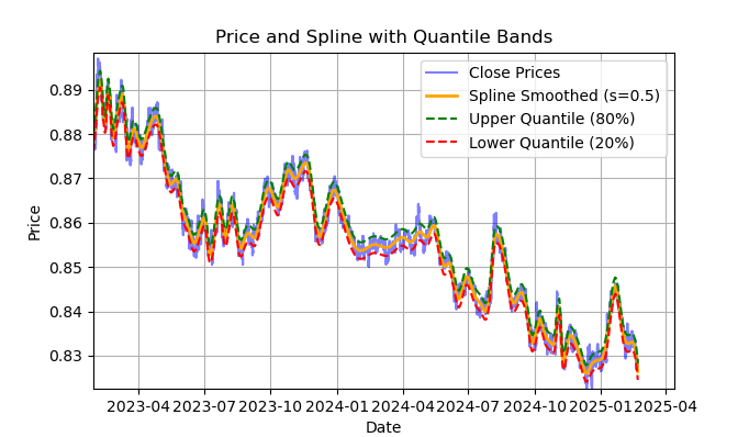
Fig. 2. Display of spline filter and bands (quantiles)

Fig. 2 shows the smoothing line of the spline filter and the 20 and 80 quantile bands. The main difference between the spline filter and the Savitzky-Golay filter is that it smooths the series using piecewise linear or non-linear functions, depending on the smoothing factor s, which is best set within the range of 0.1;1, and on the degree of the polynomial, which is usually set within the range of 1 to 3. By varying these parameters, you can visually evaluate the differences in the resulting smoothing. In the code, the degree of the polynomial k=3 is fixed, it can also be changed.

The code for constructing and visually evaluating a spline looks like this:

import pandas as pd
from scipy.interpolate import UnivariateSpline
import matplotlib.pyplot as plt

def plot_close_filter_quantiles(dataset, rolling=200, quantiles=[0.2, 0.8]):
    """
    Plots close prices with spline smoothing and quantile bands.

    Args:
        dataset (pd.DataFrame): DataFrame with 'close' column and datetime index.
        rolling (int, optional): Rolling window size for spline smoothing. 
                                  Defaults to 200.
        quantiles (list, optional): Quantiles for band calculation. 
                                     Defaults to [0.2, 0.8].
        s (float, optional): Smoothing factor for UnivariateSpline. 
                             Adjusts the spline stiffness. Defaults to 1000.
    """
    
    # Create spline smoothing
    # Convert datetime index to numerical values (Unix timestamps)
    numerical_index = pd.to_numeric(dataset.index)
    
    # Create spline smoothing using the numerical index
    spline = UnivariateSpline(numerical_index, dataset['close'], k=3, s=rolling)  
    smoothed = spline(numerical_index)
    
    # Calculate difference between prices and filter
    lvl = dataset['close'] - smoothed
    
    # Get quantile values
    q_low, q_high = lvl.quantile(quantiles).tolist()
    
    # Calculate bands based on quantiles
    upper_band = smoothed + q_high
    lower_band = smoothed + q_low
    
    # Create plot
    plt.figure(figsize=(14, 7))
    plt.plot(dataset.index, dataset['close'], label='Close Prices', color='blue', alpha=0.5)
    plt.plot(dataset.index, smoothed, label=f'Spline Smoothed (s={rolling})', color='orange', linewidth=2)
    plt.plot(dataset.index, upper_band, label=f'Upper Quantile ({quantiles[1]*100:.0f}%)', 
             color='green', linestyle='--')
    plt.plot(dataset.index, lower_band, label=f'Lower Quantile ({quantiles[0]*100:.0f}%)', 
             color='red', linestyle='--')
    
    # Configure display
    plt.title('Price and Spline with Quantile Bands')
    plt.xlabel('Date')
    plt.ylabel('Price')
    plt.legend()
    plt.grid(True)
    plt.show()

A detailed description of the entire calculate_labels_mean_reversion function, for a full understanding of the trade labeling code, is provided below.

calculate_labels_mean_reversion function:

Input data:

• close - array of close prices
• lvl - array of price deviations from the smoothed series
• markup - in %
• min_l - minimum number of candles to test the condition
• max_l - maximum number of candles to test the condition
• an array of quantiles defining signal zones

Logic:

1. Initialization: Create an empty 'labels' array of len(close) - max_l length to store signals. The length has been shortened to account for future price values. 

2. Loop through prices: For each close[i] price with index i from 0 to len(close) — max_l - 1:

• Define 'rand' random number between min_l and max_l.
• Get the curr_pr current price, the curr_lvl current deviation and the future_pr future price for 'rand' candles ahead. 
• Sell signal: If curr_lvl is greater than the (q[1]) upper quantile and the future_pr future price taking into account the 'markup' is less than the current price, set labels[i] = 1.0.
• Buy singal: If curr_lvl is less than the lower quantile (q[0]) and the future_pr future price minus the markup is greater than the current price, set labels[i] = 0.0.
• No signal: In other cases, set labels[i] = 2.0.

3. Return result: Return the 'labels' array with signals.

get_labels_mean_reversion function:

Input data:

• dataset: DataFrame with financial data containing the 'close' column
• markup - in %
• min_l - minimum number of candles to test the condition
• max_l - maximum number of candles to test the condition
• rolling - smoothing parameter (window size or ratio)
• quantiles - quantiles for determining signal zones
• method - smoothing method ('mean', 'spline', 'savgol')
• shift - shift of the smoothed series

Logic:

1. Calculation of deviations: Calculate the lvl deviations from the smoothed price series (close) depending on the selected 'method':

• mean - deviation from the moving average 
• spline - deviation from the spline-smoothed curve
• savgol - deviation from the smoothed Savitzky-Golay filter

2. Removing gaps: Remove rows with gaps (NaN) from the dataset.

3. Calculating quantiles: Calculating q quantiles for lvl deviations.

4. Data preparation: Extract arrays of close prices and lvl deviations from the 'dataset'.

5. Signal calculation:

• Call the calculate_labels_mean_reversion function with the prepared data to obtain the 'labels' array with signals.

6. DataFrame handling:

• Truncate 'dataset' up to 'labels'.
• Add 'labels' as the new 'labels' column to 'dataset'.
• Remove rows with gaps (NaN) from the 'dataset'.
• Remove strings where 'labels' is equal to 2.0 (no signal).
• Remove the lvl column.

7. Return result: Return a modified 'dataset' with the Buy and Sell signals in the 'labels' column

For variety, let's implement a version of the same sampler that checks conditions for several filters with different periods, and not just one. If all conditions for all filters are met and they have the same direction (buy or sell), and the transaction is profitable over a period of n bars into the future, then it satisfies the labeling conditions; otherwise, it is ignored and removed from the training sample.

@njit
def calculate_labels_mean_reversion_multi(close_data, lvl_data, q, markup, min_l, max_l, windows):
    labels = []
    for i in range(len(close_data) - max_l):
        rand = random.randint(min_l, max_l)
        curr_pr = close_data[i]
        future_pr = close_data[i + rand]

        buy_condition = True
        sell_condition = True
        qq = 0
        for rolling in windows:
            curr_lvl = lvl_data[i, qq]            
            if not (curr_lvl >= q[qq][1]):
                sell_condition = False
            if not (curr_lvl <= q[qq][0]):
                buy_condition = False
            qq+=1
    
        if sell_condition and (future_pr + markup) < curr_pr:
            labels.append(1.0)
        elif buy_condition and (future_pr - markup) > curr_pr:
            labels.append(0.0)
        else:
            labels.append(2.0)
    return labels

def get_labels_mean_reversion_multi(dataset, markup, min_l=1, max_l=15, windows=[0.2, 0.3, 0.5], quantiles=[.45, .55]):
    """
    Generates labels for a financial dataset based on mean reversion 
    principles using multiple smoothing windows.

    This function calculates trading signals (buy/sell) based on the deviation 
    of the price from smoothed price trends calculated using multiple spline 
    smoothing factors (windows). It identifies potential buy opportunities when 
    the price deviates significantly below its smoothed trends across multiple
    timeframes.

    Args:
        dataset (pd.DataFrame): DataFrame containing financial data with a 'close' column.
        markup (float): The percentage markup used to determine buy signals.
        min_l (int, optional): Minimum number of consecutive days the markup must hold. Defaults to 1.
        max_l (int, optional): Maximum number of consecutive days the markup is considered. Defaults to 15.
        windows (list, optional): List of smoothing factors (rolling window equivalents) 
                                   for spline calculations. Defaults to [0.2, 0.3, 0.5].
        quantiles (list, optional): Quantiles to define the "reversion zone". Defaults to [.45, .55].

    Returns:
        pd.DataFrame: The original DataFrame with a new 'labels' column and filtered rows:
                       - 'labels' column: 
                            - 0: Buy
                            - 1: Sell
                       - Rows where 'labels' is 2 (sell signal) are removed.
                       - Rows with missing values (NaN) are removed. 
    """

    q = []  # Initialize an empty list to store quantiles for each window
    lvl_data = np.empty((dataset.shape[0], len(windows)))  # Initialize a 2D array to store price deviation data

    # Calculate price deviation from smoothed trends for each window
    for i, rolling in enumerate(windows):
        x = np.array(range(dataset.shape[0]))  # Create an array of x-values (time index)
        y = dataset['close'].values  # Extract closing prices
        spl = UnivariateSpline(x, y, k=3, s=rolling)  # Create a spline smoothing function
        yHat = spl(np.linspace(min(x), max(x), num=x.shape[0]))  # Generate smoothed price data
        lvl_data[:, i] = dataset['close'] - yHat  # Calculate price deviation from smoothed prices
        q.append(np.quantile(lvl_data[:, i], quantiles).tolist())  # Calculate and store quantiles

    dataset = dataset.dropna()  # Remove NaN values before proceeding

    close_data = dataset['close'].values  # Extract closing prices 

    # Calculate buy/hold labels using multiple price deviation series
    labels = calculate_labels_mean_reversion_multi(close_data, lvl_data, q, markup, min_l, max_l, windows)

    # Process the dataset and labels
    dataset = dataset.iloc[:len(labels)].copy()  # Trim the dataset to match label length
    dataset['labels'] = labels  # Add the calculated labels as a new column
    dataset = dataset.dropna()  # Remove rows with NaN values
    dataset = dataset.drop(dataset[dataset.labels == 2.0].index)  # Remove sell signals (if any)
    
    return dataset

Finally, let's write another mean reversion trade labeling function that calculates quantiles in a sliding window of a given period, rather than over the entire history of observations. This will help smooth out the impact of variable volatility in price deviation from the mean.

@njit
def calculate_labels_mean_reversion_v(close_data, lvl_data, volatility_group, quantile_groups, markup, min_l, max_l):
    labels = []
    for i in range(len(close_data) - max_l):
        rand = random.randint(min_l, max_l)
        curr_pr = close_data[i]
        curr_lvl = lvl_data[i]
        curr_vol_group = volatility_group[i]
        future_pr = close_data[i + rand]

        q = quantile_groups[curr_vol_group]

        if curr_lvl > q[1] and (future_pr + markup) < curr_pr:
            labels.append(1.0)
        elif curr_lvl < q[0] and (future_pr - markup) > curr_pr:
            labels.append(0.0)
        else:
            labels.append(2.0)
    return labels

def get_labels_mean_reversion_v(dataset, markup, min_l=1, max_l=15, rolling=0.5, quantiles=[.45, .55], method='spline', shift=1, volatility_window=20) -> pd.DataFrame:
    """
    Generates trading labels based on mean reversion principles, incorporating
    volatility-based adjustments to identify buy opportunities.

    This function calculates trading signals (buy/sell), taking into account the 
    volatility of the asset. It groups the data into volatility bands and calculates 
    quantiles for each band. This allows for more dynamic "reversion zones" that 
    adjust to changing market conditions.

    Args:
        dataset (pd.DataFrame): DataFrame containing financial data with a 'close' column.
        markup (float): The percentage markup used to determine buy signals.
        min_l (int, optional): Minimum number of consecutive days the markup must hold. Defaults to 1.
        max_l (int, optional): Maximum number of consecutive days the markup is considered. Defaults to 15.
        rolling (float, optional): Rolling window size or spline smoothing factor (see 'method'). 
                                     Defaults to 0.5.
        quantiles (list, optional): Quantiles to define the "reversion zone". Defaults to [.45, .55].
        method (str, optional): Method for calculating the price deviation:
                                 - 'mean': Deviation from the rolling mean.
                                 - 'spline': Deviation from a smoothed spline.
                                 - 'savgol': Deviation from a Savitzky-Golay filter.
                                 Defaults to 'spline'.
        shift (int, optional): Shift the smoothed price data (lag/lead effect). Defaults to 1.
        volatility_window (int, optional): Window size for calculating volatility. Defaults to 20.

    Returns:
        pd.DataFrame: The original DataFrame with a new 'labels' column and filtered rows:
                       - 'labels' column: 
                            - 0: Buy
                            - 1: Sell
                       - Rows where 'labels' is 2 (no signal) are removed.
                       - Rows with missing values (NaN) are removed.
                       - Temporary 'lvl', 'volatility', 'volatility_group' columns are removed.
    """

    # Calculate Volatility
    dataset['volatility'] = dataset['close'].pct_change().rolling(window=volatility_window).std()
    
    # Divide into 20 groups by volatility 
    dataset['volatility_group'] = pd.qcut(dataset['volatility'], q=20, labels=False)
    
    # Calculate price deviation ('lvl') based on the chosen method
    if method == 'mean':
        dataset['lvl'] = (dataset['close'] - dataset['close'].rolling(rolling).mean())
    elif method == 'spline':
        x = np.array(range(dataset.shape[0]))
        y = dataset['close'].values
        spl = UnivariateSpline(x, y, k=3, s=rolling)
        yHat = spl(np.linspace(min(x), max(x), num=x.shape[0]))
        yHat_shifted = np.roll(yHat, shift=shift) # Apply the shift 
        dataset['lvl'] = dataset['close'] - yHat_shifted
        dataset = dataset.dropna() 
    elif method == 'savgol':
        smoothed_prices = savgol_filter(dataset['close'].values, window_length=rolling, polyorder=5)
        dataset['lvl'] = dataset['close'] - smoothed_prices

    dataset = dataset.dropna()
    
    # Calculate quantiles for each volatility group
    quantile_groups = {}
    for group in range(20):
        group_data = dataset[dataset['volatility_group'] == group]['lvl']
        quantile_groups[group] = group_data.quantile(quantiles).to_list()
    
    # Prepare data for label calculation (potentially using Numba)
    close_data = dataset['close'].values
    lvl_data = dataset['lvl'].values
    volatility_group = dataset['volatility_group'].values

    # Calculate buy/sell labels 
    labels = calculate_labels_mean_reversion_v(close_data, lvl_data, volatility_group, quantile_groups, markup, min_l, max_l)
    
    # Process dataset and labels
    dataset = dataset.iloc[:len(labels)].copy()
    dataset['labels'] = labels
    dataset = dataset.dropna()
    dataset = dataset.drop(dataset[dataset.labels == 2.0].index) # Remove sell signals
    
    # Remove temporary columns and return
    return dataset.drop(columns=['lvl', 'volatility', 'volatility_group'])

So, we already have a number of trade markers to experiment with. Approaches can be combined and new ones can be created.

The full list of the above-described trade samplers from the labeling_lib.py library is presented below. Based on these, you can modify old ones and create new ones, depending on how well you understand market patterns and what strategy you want to have as a result. The module also contains other custom trade samplers, but they are not related to mean reversion strategies and are therefore not described in this article.

# FILTERING BASED LABELING W/O RESTRICTIONS
def get_labels_filter(dataset, rolling=200, quantiles=[.45, .55], polyorder=3) -> pd.DataFrame
def get_labels_multiple_filters(dataset, rolling_periods=[200, 400, 600], quantiles=[.45, .55], window=100, polyorder=3) -> pd.DataFrame
def get_labels_filter_bidirectional(dataset, rolling1=200, rolling2=200, quantiles=[.45, .55], polyorder=3) -> pd.DataFrame:

# MEAN REVERSION WITH RESTRICTIONS BASED LABELING
def get_labels_mean_reversion(dataset, markup, min_l=1, max_l=15, rolling=0.5, quantiles=[.45, .55], method='spline', shift=0) -> pd.DataFrame
def get_labels_mean_reversion_multi(dataset, markup, min_l=1, max_l=15, windows=[0.2, 0.3, 0.5], quantiles=[.45, .55]) -> pd.DataFrame
def get_labels_mean_reversion_v(dataset, markup, min_l=1, max_l=15, rolling=0.5, quantiles=[.45, .55], method='spline', shift=1, volatility_window=20) -> pd.DataFrame:

It is time to move on to the second part of the article, namely clustering market modes, and then combining both approaches to create trading systems based on mean reversion.

What to cluster and why is it necessary?

Before clustering anything, we need to decide why we need to do it at all. Let's imagine a price chart that has a trend, a flat, periods of high and low volatility, various patterns, and other features. That is, the price chart is not something uniform, where the same patterns are present. One could even say that at different periods of time there are or may be different patterns that disappear at other time intervals.

Clustering allows you to divide the original time series into several states based on certain characteristics, so that each of these states describes similar observations. This can make the task of building a trading system easier, since training will occur on more homogeneous, similar data. At least, that is how one can imagine it. Naturally, the trading system will no longer operate over the entire historical period, but rather over a selected portion of it, made up of different points in time, the values of which fall within a given cluster.

After clustering, only selected examples can be labeled, that is, assigned unique class labels, to build the final model. If a cluster contains homogeneous data with similar observations, then its labeling should become more homogeneous and, subsequently, more predictable. You can take multiple clusters of data, label each of them separately, then train machine learning models on the data from each cluster and test them on the training and test data. If a cluster is found that allows the model to learn well, that is, to generalize and predict on new data, the task of building a trading system can be considered practically completed.

Clustering financial time series to identify market modes

Before reading this section, it might be useful to familiarize yourself with the different types of clustering algorithms that were described in the previous article. It also provides a comparative table of various clustering algorithms and their test results. For this article, I have chosen the conventional k-means clustering algorithm as the fastest and most efficient one.

At the stage of creating features using the get_features function, we need to provide for the possibility of the presence in the dataset of exactly those features, by which clustering will be carried out. I propose to consider three basic options to start from. If you have any other features that you think describe market regimes well, feel free to use them. To do this, it is necessary to add their calculation to the feature generation function, and they must contain "meta_feature" symbols in their name, to further separate them from the main features.

def get_features(data: pd.DataFrame) -> pd.DataFrame:
    pFixed = data.copy()
    pFixedC = data.copy()
    count = 0

    for i in hyper_params['periods']:
        pFixed[str(count)] = pFixedC.rolling(i).mean()
        count += 1
    
    for i in hyper_params['periods_meta']:
        pFixed[str(count)+'meta_feature'] = pFixedC.rolling(i).skew()
        count += 1

    # for i in hyper_params['periods_meta']:
    #     pFixed[str(count)+'meta_feature'] = pFixedC.rolling(i).std()
    #     count += 1

    # for i in hyper_params['periods_meta']:
    #     pFixed[str(count)+'meta_feature'] = pFixedC - pFixedC.rolling(i).mean()
    #     count += 1

    return pFixed.dropna()

In the first loop, all the features specified in the 'periods' list are calculated. These are the main features that will be used to train the main machine learning model that predicts buy or sell trades. In this case, these are simple moving averages with different periods.

In the second loop, the features specified in the 'periods_meta' list are calculated. These are precisely the features that will participate in clustering market regimes. By default, clustering will be calculated based on the skew of quotes in the sliding window. The commented out fields correspond to the calculation of features based on the standard deviation in the sliding window, or based on price increments. The selection of features is carried out empirically, through enumeration of various options. Experiments have shown that skew-based (asymmetry-based) clustering separates data well, so it will be used in this article.

Skewness (or asymmetry) in distributions is a characteristic that describes the degree, to which a data distribution is not symmetrical about its mean. Skewness measures how much a distribution deviates from symmetry (e.g., a normal distribution). Skewness is measured using the ratio of asymmetry (skewness). Skew clustering allows one to identify groups of data with similar distribution characteristics, which helps identify these modes. For example, a positive slope may indicate periods with rare but strong price surges (for example, during crises), while a negative slope may indicate periods with smoother changes.

After the features have been formed, the final dataset is passed to the function that performs clustering. The function also adds a new "clusters" column, which contains the cluster numbers.

def clustering(dataset, n_clusters: int) -> pd.DataFrame:
    data = dataset[(dataset.index < hyper_params['forward']) & (dataset.index > hyper_params['backward'])].copy()
    meta_X = data.loc[:, data.columns.str.contains('meta_feature')]
    data['clusters'] = KMeans(n_clusters=n_clusters).fit(meta_X).labels_
    return data

To prevent "peeking", data is truncated before and after the dates specified in the algorithm settings so that clustering is performed only on the data that will be used in the model training. The code also includes a selection of features for clustering, which are selected using the 'meta_feature' keyword in the feature column name.

All the algorithm hyperparameters are stored in a dictionary, the data from which will be used to create features, select the training period, and so on.

hyper_params = {
    'symbol': 'EURGBP_H1',
    'export_path': '/Users/dmitrievsky/Library/Containers/com.isaacmarovitz.Whisky/Bottles/54CFA88F-36A3-47F7-915A-D09B24E89192/drive_c/Program Files/MetaTrader 5/MQL5/Include/Mean reversion/',
    # 'export_path': '/Users/dmitrievsky/Library/Containers/com.isaacmarovitz.Whisky/Bottles/54CFA88F-36A3-47F7-915A-D09B24E89192/drive_c/Program Files (x86)/RoboForex MT4 Terminal/MQL4/Include/',
    'model_number': 0,
    'markup': 0.00010,
    'stop_loss':  0.02000,
    'take_profit': 0.00200,
    'periods': [i for i in range(5, 300, 30)],
    'periods_meta': [10],
    'backward': datetime(2000, 1, 1),
    'forward': datetime(2021, 1, 1),
    'n_clusters': 10,
    'rolling': 200,
}

• The name of the file on disk that contains the symbol quotes
• Export path for exporting trained models to the #include directory of the MetaTrader 5 terminal
• Model ID to distinguish them after export when there is a need to export multiple models
• Markup, which should take into account the average spread and commission, in points. For more accurate labeling of deals and subsequent testing on history.
• Stop loss supported by the fast custom tester
• Take profit
• List of periods for calculating the main features. Each individual element of the list represents a period for a separate feature. The more elements, the more features.
• List of periods for features that participate in clustering.
• Initial date of model training
• End date of model training
• The number of clusters (modes) the data will be divided into
• Sliding window parameter for filter smoothing

Now let's put it all together, look at the main model training loop, and analyze all the stages of both preprocessing and training itself.

# LEARNING LOOP
dataset = get_features(get_prices())
models = []
for i in range(1):
    data = clustering(dataset, n_clusters=hyper_params['n_clusters'])
    sorted_clusters = data['clusters'].unique()
    sorted_clusters.sort()
    for clust in sorted_clusters:
        clustered_data = data[data['clusters'] == clust].copy()
        if len(clustered_data) < 500:
            print('too few samples: {}'.format(len(clustered_data)))
            continue
    
        clustered_data = get_labels_filter(clustered_data, 
                                           rolling=hyper_params['rolling'],
                                           quantiles=[0.45, 0.55],
                                           polyorder=3
                                            )

        print(f'Iteration: {i}, Cluster: {clust}')
        clustered_data = clustered_data.drop(['close', 'clusters'], axis=1)

        meta_data = data.copy()
        meta_data['clusters'] = meta_data['clusters'].apply(lambda x: 1 if x == clust else 0)
        models.append(fit_final_models(clustered_data, meta_data.drop(['close'], axis=1)))

First, a dataset is created that contains prices and features. Creating features was described above. Then the 'models' list is created, which will store the already trained models. Next we have a choice: how many training iterations will be performed in the loop. The default is one iteration. If you need to train multiple models, specify their number in the range() iterator. 

After this, the original dataset is clustered and each example is assigned a cluster number. If 10 n_clusters are specified in the hyperparameters, then this parameter is passed to the function, and clustering into 10 clusters occurs. Experiments have shown that 10 clusters is the optimal number of market modes, but of course one can experiment with this parameter. 

Next, the final number of clusters is determined, their serial numbers are sorted in ascending order, and then, for each cluster number, only those rows from the dataset that correspond to it are selected. We are not interested in clusters that have too few observations, so we check to make sure there are at least 500 examples.

The next step is to call the deal labeling function for the currently selected cluster. In this case, I took the very first labeling function get_labels_filter this article started with. After the deals are labeled, the data is divided into two datasets. The first dataset will contain the main features and labels, and the second will contain the meta features used for clustering, as well as labels 0 and 1. One means that the data corresponds to the selected cluster, and zeros mean that it is any cluster other than the selected one. After all, we want the trading system to trade only in a specific market mode.

Thus, the first model will learn to predict the direction of the trade, and the second model will predict when they can be opened and when they should not.

Let's now look at the fit_final_models function itself, which takes two datasets for two final models and trains the CatBoost algorithm on them.

def fit_final_models(clustered, meta) -> list:
    # features for model\meta models. We learn main model only on filtered labels 
    X, X_meta = clustered[clustered.columns[:-1]], meta[meta.columns[:-1]]
    X = X.loc[:, ~X.columns.str.contains('meta_feature')]
    X_meta = X_meta.loc[:, X_meta.columns.str.contains('meta_feature')]
    
    # labels for model\meta models
    y = clustered['labels']
    y_meta = meta['clusters']
    
    y = y.astype('int16')
    y_meta = y_meta.astype('int16')

    # train\test split
    train_X, test_X, train_y, test_y = train_test_split(
        X, y, train_size=0.7, test_size=0.3, shuffle=True)
    
    train_X_m, test_X_m, train_y_m, test_y_m = train_test_split(
        X_meta, y_meta, train_size=0.7, test_size=0.3, shuffle=True)


    # learn main model with train and validation subsets
    model = CatBoostClassifier(iterations=1000,
                               custom_loss=['Accuracy'],
                               eval_metric='Accuracy',
                               verbose=False,
                               use_best_model=False,
                               task_type='CPU',
                               thread_count=-1)
    model.fit(train_X, train_y, eval_set=(test_X, test_y),
              early_stopping_rounds=30, plot=False)
    
    # learn meta model with train and validation subsets
    meta_model = CatBoostClassifier(iterations=500,
                                    custom_loss=['F1'],
                                    eval_metric='F1',
                                    verbose=False,
                                    use_best_model=True,
                                    task_type='CPU',
                                    thread_count=-1)
    meta_model.fit(train_X_m, train_y_m, eval_set=(test_X_m, test_y_m),
              early_stopping_rounds=25, plot=False)

    
    R2 = test_model([model, meta_model], hyper_params['stop_loss'], hyper_params['take_profit'])
    if math.isnan(R2):
        R2 = -1.0
        print('R2 is fixed to -1.0')
    print('R2: ' + str(R2))

    return [R2, model, meta_model]

Training stages:

1. Data preparation:

• From the 'clustered' and 'meta' input dataframes, (X, X_meta) features and (y, y_meta) labels are extracted.
• Label data types are converted to int16. This is necessary for seamless conversion of the model to ONNX format.
• The data is split into training and test sets using train_test_split.

2. Training the main model:

• The CatBoostClassifier object is created with the given hyperparameters.
• The model is trained on the (train_X, train_y) training data using the (test_X, test_y) validation set for early stop.

3. Meta model training:

• A CatBoostClassifier object is created for the meta model with the given hyperparameters.
• The meta model is trained similarly to the main model, using the corresponding training and test data.

4. Model evaluation:

• The trained models (model, meta_model) are passed to the test_model function along with the stop_loss and take_profit parameters to evaluate their performance.
• The returned R2 value represents the performance metric of the model.

5. Handling R2 and returning the result:

• If R2 is NaN, it is replaced with -1.0.
• The value of R2 is displayed on the screen.
• The function returns the list containing R2 and trained models (model, meta_model). 

For each cluster, the output is two trained classifier models, ready for final visual test and export to the MetaTrader 5 terminal. It should be remembered that for each training iteration, as many pairs of models are created as there are clusters specified in the hyperparameters. This number should be multiplied by the number of iterations to get an idea of how many pairs of models will be produced in total. For example, if 10 clusters and 10 iterations are specified, then the output will be 100 pairs of models, excluding those that did not pass the filtering for the minimum number of examples.

Training and testing models. Testing the algorithm

For more convenient use of the algorithm, it is advisable to run it in the interactive Python environment string by string. Then we can change the hyperparameters and experiment with different samplers. Or we can transfer all the code to the .ipynb format to run in IPython via a laptop. If you are going to run the entire script, you will still have to edit it to customize the parameters.

I suggest testing each of the labeling functions by running 10 iterations for each. The remaining parameters will be the same as those specified in the attached script.

Once the training loop is launched, the training results on each iteration for each data cluster are displayed.

R2: 0.9815970951474068
Iteration: 9, Cluster: 5
R2: 0.9914890771969395
Iteration: 9, Cluster: 6
R2: 0.9450681335265942
Iteration: 9, Cluster: 7
R2: 0.9631330369697314
Iteration: 9, Cluster: 8
R2: 0.9680380185183347
Iteration: 9, Cluster: 9
R2: 0.8203651933893291

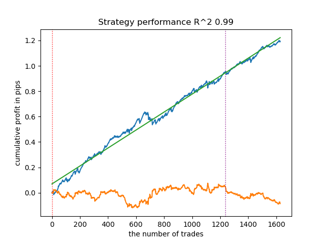
We can then sort all results in ascending R^2 order to select the best one. We can also visually evaluate the balance curve in the tester.

models.sort(key=lambda x: x[0])
test_model(models[-1][1:], hyper_params['stop_loss'], hyper_params['take_profit'], plt=True)

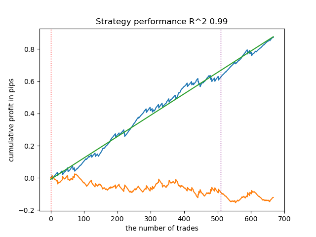
The highlighted one means that the first model from the end (i.e. the one with the highest R^2) will be tested. To test the second-to-last model, you need to set -2, and so on. The tester will display a balance graph (blue) and a currency pair graph (orange), as well as a vertical line that separates the training period and new data. All models are trained from the beginning of 2010 to the beginning of 2021, this is specified in the hyperparameters. You can change the training and test intervals at your discretion. The test period for all models in this article is from the beginning of 2021 to the beginning of 2025.

Testing different trade samplers

• get_labels_filter(dataset, rolling=200, quantiles=[.45, .55], polyorder=3)

Below is the best result for the get_labels_filter marker.

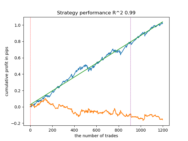
The basic marker did a good job of labeling the trades, and all the models turned out to be profitable on the new data. Let's do the same for the remaining markers and look at the results.

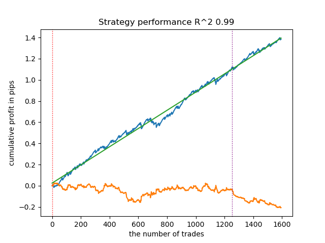
• get_labels_multiple_filters(dataset,rolling_periods=[50,100,200],quantiles=[.45,.55],window=100,polyorder=3)

Models trained on this marker's data often show an increase in the number of trades relative to the baseline. I have not experimented with the settings here because the article would have been too long.

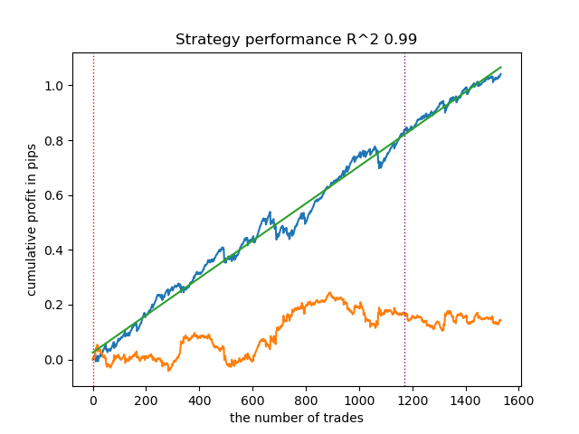
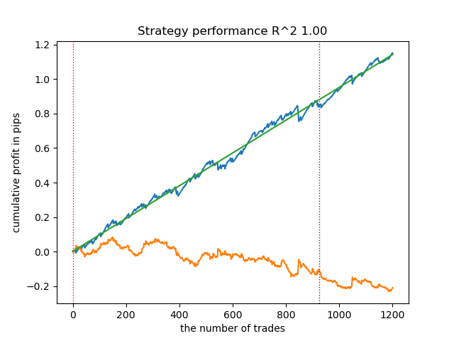
• get_labels_filter_bidirectional(dataset, rolling1=50, rolling2=200, quantiles=[.45, .55], polyorder=3)

This asymmetrical marker also demonstrated its efficiency on new data. By selecting different smoothing parameters separately for buy and sell trades, you can achieve optimal results.

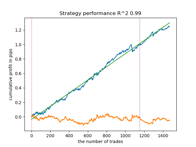
Now let's move on to markers with restrictions on strictly profitable deals. It is clear that the previous markers do not provide a smooth balance curve even during the training period, but they do capture the general patterns well. Let's see what changes if we remove losing trades from the training dataset.

• get_labels_mean_reversion(dataset, markup, min_l=1, max_l=15, rolling=0.5, quantiles=[.45, .55], method='spline', shift=0)

I tested this marker using a spline as a filter and a fixed smoothing factor of 0.5. The article does not provide tests for the Savitzky-Golay filter and the simple moving average. However, it can be seen that smoother curves can be achieved by using a deal profitability restriction.

• get_labels_mean_reversion_multi(dataset, markup, min_l=1, max_l=15, windows=[0.2, 0.3, 0.5], quantiles=[.45, .55])

This sampler is also capable of providing high-quality samples, thanks to which the model continues to trade profitably on new data.

• get_labels_mean_reversion_v(dataset, markup, min_l=1, max_l=15, rolling=0.2, quantiles=[.45, .55], method='spline', shift=0, volatility_window=20)

This algorithm is also capable of demonstrating acceptable labeling and good output models.

Conclusions on deal markers:

• When you do not know where to start and it all seems too complicated for you, use the most basic sampler that can give an acceptable result.
• If you do not get pretty images right away, remember that there are random components in the labeling of trades and the training of models. Simply rerun the algorithm a few times.
• All samplers with basic settings can produce acceptable results. For more fine-tuning, you need to focus on one of them and start selecting parameters.

Conclusions on clustering:

• Behind the scenes, multiple tests were performed on samplers without clustering, as well as clustering without using samplers. I have found that these algorithms do not work as well individually as in tandem.
• There is no need to create too many features by which clustering will be carried out. This will complicate the model and make it less robust to new data.
• The optimal number of clusters is in the range of 5-10. Too few clusters result in poor generalization ability and poor results on new data, while too many clusters result in a sharp reduction in the number of transactions.

For ease of use, uncomment the desired deal marker in the code.

# LEARNING LOOP
dataset = get_features(get_prices())
models = []
for i in range(10):
    data = clustering(dataset, n_clusters=hyper_params['n_clusters'])
    sorted_clusters = data['clusters'].unique()
    sorted_clusters.sort()
    for clust in sorted_clusters:
        clustered_data = data[data['clusters'] == clust].copy()
        if len(clustered_data) < 500:
            print('too few samples: {}'.format(len(clustered_data)))
            continue
    
        clustered_data = get_labels_filter(clustered_data, 
                                           rolling=hyper_params['rolling'],
                                           quantiles=[0.45, 0.55],
                                           polyorder=3
                                            )
        # clustered_data = get_labels_multiple_filters(clustered_data, 
        #                                              rolling_periods=[50, 100, 200], 
        #                                              quantiles=[.45, .55], 
        #                                              window=100, 
        #                                              polyorder=3)
        # clustered_data = get_labels_filter_bidirectional(clustered_data, 
        #                                                  rolling1=50, 
        #                                                  rolling2=200, 
        #                                                  quantiles=[.45, .55], 
        #                                                  polyorder=3)
        # clustered_data = get_labels_mean_reversion(clustered_data,
        #                                             markup = hyper_params['markup'],
        #                                             min_l=1, max_l=15, 
        #                                             rolling=0.5, 
        #                                             quantiles=[.45, .55], 
        #                                             method='spline', shift=0)
        # clustered_data = get_labels_mean_reversion_multi(clustered_data, 
        #                                                  markup = hyper_params['markup'], 
        #                                                  min_l=1, max_l=15, 
        #                                                  windows=[0.2, 0.3, 0.5], 
        #                                                  quantiles=[.45, .55])
        # clustered_data = get_labels_mean_reversion_v(clustered_data,
        #                                             markup = hyper_params['markup'],
        #                                             min_l=1, max_l=15, 
        #                                             rolling=0.2, 
        #                                             quantiles=[.45, .55], 
        #                                             method='spline', 
        #                                             shift=0, 
        #                                             volatility_window=100)

        print(f'Iteration: {i}, Cluster: {clust}')
        clustered_data = clustered_data.drop(['close', 'clusters'], axis=1)

        meta_data = data.copy()
        meta_data['clusters'] = meta_data['clusters'].apply(lambda x: 1 if x == clust else 0)
        models.append(fit_final_models(clustered_data, meta_data.drop(['close'], axis=1)))

# TESTING & EXPORT
models.sort(key=lambda x: x[0])
test_model(models[-1][1:], hyper_params['stop_loss'], hyper_params['take_profit'], plt=True)

Exporting trained models in MetaTrader 5 

The penultimate step includes exporting the trained models and header file to ONNX format. The export_lib.py module, attached below, contains the export_model_to_ONNX(**kwargs) function. Let's take a closer look at it.

def export_model_to_ONNX(**kwargs):
    model = kwargs.get('model')
    symbol = kwargs.get('symbol')
    periods = kwargs.get('periods')
    periods_meta = kwargs.get('periods_meta')
    model_number = kwargs.get('model_number')
    export_path = kwargs.get('export_path')

    model[1].save_model(
    export_path +'catmodel ' + symbol + ' ' + str(model_number) +'.onnx',
    format="onnx",
    export_parameters={
        'onnx_domain': 'ai.catboost',
        'onnx_model_version': 1,
        'onnx_doc_string': 'main model',
        'onnx_graph_name': 'CatBoostModel_main'
    },
    pool=None)

    model[2].save_model(
    export_path + 'catmodel_m ' + symbol + ' ' + str(model_number) +'.onnx',
    format="onnx",
    export_parameters={
        'onnx_domain': 'ai.catboost',
        'onnx_model_version': 1,
        'onnx_doc_string': 'meta model',
        'onnx_graph_name': 'CatBoostModel_meta'
    },
    pool=None)
    
    code = '#include <Math\Stat\Math.mqh>'
    code += '\n'
    code += '#resource "catmodel '+ symbol + ' '+str(model_number)+'.onnx" as uchar ExtModel_' + symbol + '_' + str(model_number) + '[]'
    code += '\n'
    code += '#resource "catmodel_m '+ symbol + ' '+str(model_number)+'.onnx" as uchar ExtModel2_' + symbol + '_' + str(model_number) + '[]'
    code += '\n\n'
    code += 'int Periods' + symbol + '_' + str(model_number) + '[' + str(len(periods)) + \
        '] = {' + ','.join(map(str, periods)) + '};'
    code += '\n'
    code += 'int Periods_m' + symbol + '_' + str(model_number) + '[' + str(len(periods_meta)) + \
        '] = {' + ','.join(map(str, periods_meta)) + '};'
    code += '\n\n'

    # get features
    code += 'void fill_arays' + symbol + '_' + str(model_number) + '( double &features[]) {\n'
    code += '   double pr[], ret[];\n'
    code += '   ArrayResize(ret, 1);\n'
    code += '   for(int i=ArraySize(Periods'+ symbol + '_' + str(model_number) + ')-1; i>=0; i--) {\n'
    code += '       CopyClose(NULL,PERIOD_H1,1,Periods' + symbol + '_' + str(model_number) + '[i],pr);\n'
    code += '       ret[0] = MathMean(pr);\n'
    code += '       ArrayInsert(features, ret, ArraySize(features), 0, WHOLE_ARRAY); }\n'
    code += '   ArraySetAsSeries(features, true);\n'
    code += '}\n\n'

    # get features
    code += 'void fill_arays_m' + symbol + '_' + str(model_number) + '( double &features[]) {\n'
    code += '   double pr[], ret[];\n'
    code += '   ArrayResize(ret, 1);\n'
    code += '   for(int i=ArraySize(Periods_m' + symbol + '_' + str(model_number) + ')-1; i>=0; i--) {\n'
    code += '       CopyClose(NULL,PERIOD_H1,1,Periods_m' + symbol + '_' + str(model_number) + '[i],pr);\n'
    code += '       ret[0] = MathSkewness(pr);\n'
    code += '       ArrayInsert(features, ret, ArraySize(features), 0, WHOLE_ARRAY); }\n'
    code += '   ArraySetAsSeries(features, true);\n'
    code += '}\n\n'

    file = open(export_path + str(symbol) + ' ONNX include' + ' ' + str(model_number) + '.mqh', "w")
    file.write(code)

    file.close()
    print('The file ' + 'ONNX include' + '.mqh ' + 'has been written to disk')

The function should receive a list of arguments, such as:

• model = models[-1]— a list of two trained models, which was pre-populated with models from different training iterations. Similarly to the tester, the -1 index will correspond to the model with the highest R^2, the -2 index will be the second model by its score, and so on. If you like a particular model during visual testing, then use the same index when exporting.
• symbol = hyper_params['symbol'] — symbol name, such as EURGBP_H1, specified in the hyperparameters. This name will be added when exporting models to differentiate models for different symbols.
• periods = hyper_params['periods']— a list of periods of the main model's features.
• periods_meta = hyper_params['periods_meta']  — a list of periods of features of an additional model that determines the current market mode.
• model_number = hyper_params['model_number']— model number, if you export many models and do not want them to be overwritten. Added to model names.

• export_path = hyper_params['export_path']— path to the terminal 'include' folder or its subdirectory for saving files to disk.

The function saves both models in the .onnx format and generates a header file through which these models are called and features are calculated for them. It should be noted that the calculation of features is carried out directly in the terminal, so it is necessary to ensure that it is identical to their calculation in the Python script. From the code, you can see that the fill_arrays function calculates the moving averages for the first model, and the fill_arrays_m function calculates the price skew for the second one. If you change the features in the Python script, then change their calculation in this function or in the header file itself.

An example of calling the function itself to save models to disk is shown below.

export_model_to_ONNX(model = models[-1],
                     symbol = hyper_params['symbol'],
                     periods = hyper_params['periods'],
                     periods_meta = hyper_params['periods_meta'],
                     model_number = hyper_params['model_number'],
                     export_path = hyper_params['export_path'])

Building a trading bot that uses ONNX models to execute trading operations

Let's assume that we have trained and selected a visually pleasing model using the custom tester, for example the following one:

Now we need to call the export function in the terminal.

After exporting the model, 3 files will appear in the include/mean reversion/ folder of the MetaTrader 5 terminal (in my case, a subdirectory is used to avoid confusion among other models):

• catmodel EURGBP_H1 0.onnx  — main model that provides buy and sell signals
• catmodel_m EURGBP_H1 0.onnx  — additional model that allows or prohibits trading
• EURGBP_H1 ONNX include 0.mqh  — header file that imports these models and calculates features.

ONNX model names always begin with the word "catmodel", which stands for catboost model, followed by the symbol name and timeframe. The additional model is marked with the _m suffix standing for 'meta model'. The header file name always starts with the trade symbol and ends with the model number, which is specified during export, so that new exported models do not overwrite each other unless necessary.

Let's look at the contents of the .mqh file.

#include <Math\Stat\Math.mqh>
#resource "catmodel EURGBP_H1 0.onnx" as uchar ExtModel_EURGBP_H1_0[]
#resource "catmodel_m EURGBP_H1 0.onnx" as uchar ExtModel2_EURGBP_H1_0[]

int PeriodsEURGBP_H1_0[10] = {5,35,65,95,125,155,185,215,245,275};
int Periods_mEURGBP_H1_0[1] = {10};

void fill_araysEURGBP_H1_0( double &features[]) {
   double pr[], ret[];
   ArrayResize(ret, 1);
   for(int i=ArraySize(PeriodsEURGBP_H1_0)-1; i>=0; i--) {
       CopyClose(NULL,PERIOD_H1,1,PeriodsEURGBP_H1_0[i],pr);
       ret[0] = MathMean(pr);
       ArrayInsert(features, ret, ArraySize(features), 0, WHOLE_ARRAY); }
   ArraySetAsSeries(features, true);
}

void fill_arays_mEURGBP_H1_0( double &features[]) {
   double pr[], ret[];
   ArrayResize(ret, 1);
   for(int i=ArraySize(Periods_mEURGBP_H1_0)-1; i>=0; i--) {
       CopyClose(NULL,PERIOD_H1,1,Periods_mEURGBP_H1_0[i],pr);
       ret[0] = MathSkewness(pr);
       ArrayInsert(features, ret, ArraySize(features), 0, WHOLE_ARRAY); }
   ArraySetAsSeries(features, true);
}

First, a library of mathematical calculations is connected, which will be needed to calculate the mean and skew, and potentially also for other moments of distributions and other mathematical calculations if it is necessary to change the calculation of features. Next, we load our two ONNX models as resources that will be used to generate trading signals. After this, arrays with periods for calculating features are declared, which will be the input data for the main and meta models.

The remaining two functions fill the arrays with feature values. Let me remind you that these files are created when exporting models from a Python script and do not need to be written from scratch each time. It is enough to simply connect to a trading EA. This is very convenient in cases where you want to retrain the model after some time, then simply export it to the terminal, the model is overwritten with a more recent one, and you recompile the bot without making any changes to the code. The sheer volume of code can be daunting at first, but in practice, training is as simple as running the script and then compiling the bot, which can take just a few minutes.

Now we need to create a trading EA, to which this header file will connect and initialize ONNX models.

#include <Mean reversion/EURGBP_H1 ONNX include 0.mqh>
#include <Trade\Trade.mqh>
#include <Trade\AccountInfo.mqh>
#property strict
#property copyright "Copyright 2025, Dmitrievsky max."
#property link      "https://www.mql5.com/ru/users/dmitrievsky"
#property version   "1.0"

CTrade mytrade;
CPositionInfo myposition;

input bool Allow_Buy = true;           //Allow BUY
input bool Allow_Sell = true;          //Allow SELL
double main_threshold = 0.5;
double meta_threshold = 0.5;
sinput double   MaximumRisk=0.001;     //Progressive lot coefficient
sinput double   ManualLot=0.01;        //Fixed lot, set 0 if progressive
sinput ulong    OrderMagic = 57633493; //Orders magic
input int max_orders = 3;              //Max positions number
input int orders_time_delay = 5;       //Time delay between positions
input int max_spread = 20;             //Max spread
input int stoploss = 2000;             //Stop loss
input int takeprofit = 200;            //Take profit
input string comment = "mean reversion bot";

static datetime last_time = 0;
#define Ask SymbolInfoDouble(_Symbol, SYMBOL_ASK)
#define Bid SymbolInfoDouble(_Symbol, SYMBOL_BID)


const long  ExtInputShape [] = {1, ArraySize(PeriodsEURGBP_H1_0)};
const long  ExtInputShape2 [] = {1, ArraySize(Periods_mEURGBP_H1_0)};
long     ExtHandle = INVALID_HANDLE, ExtHandle2 = INVALID_HANDLE;

//+------------------------------------------------------------------+
//| Expert initialization function                                   |
//+------------------------------------------------------------------+
int OnInit()
  {
   mytrade.SetExpertMagicNumber(OrderMagic);

   ExtHandle = OnnxCreateFromBuffer(ExtModel_EURGBP_H1_0, ONNX_DEFAULT);
   ExtHandle2 = OnnxCreateFromBuffer(ExtModel2_EURGBP_H1_0, ONNX_DEFAULT);

   if(ExtHandle == INVALID_HANDLE || ExtHandle2 == INVALID_HANDLE)
     {
      Print("OnnxCreateFromBuffer error ", GetLastError());
      return(INIT_FAILED);
     }

   if(!OnnxSetInputShape(ExtHandle, 0, ExtInputShape))
     {
      Print("OnnxSetInputShape 1 failed, error ", GetLastError());
      OnnxRelease(ExtHandle);
      return(-1);
     }

   if(!OnnxSetInputShape(ExtHandle2, 0, ExtInputShape2))
     {
      Print("OnnxSetInputShape 2 failed, error ", GetLastError());
      OnnxRelease(ExtHandle2);
      return(-1);
     }

   const long output_shape[] = {1};
   if(!OnnxSetOutputShape(ExtHandle, 0, output_shape))
     {
      Print("OnnxSetOutputShape 1 error ", GetLastError());
      return(INIT_FAILED);
     }
   if(!OnnxSetOutputShape(ExtHandle2, 0, output_shape))
     {
      Print("OnnxSetOutputShape 2 error ", GetLastError());
      return(INIT_FAILED);
     }

   return(INIT_SUCCEEDED);
  }
//+------------------------------------------------------------------+
//| Expert deinitialization function                                 |
//+------------------------------------------------------------------+
void OnDeinit(const int reason)
  {
//---
   OnnxRelease(ExtHandle);
   OnnxRelease(ExtHandle2);
  }

The most important thing is to correctly initialize the dimensions of the input arrays for each model. It is equal to the size of the array in the header file that contains the period values for feature calculation. There are as many signs as there are period values.

The output dimension for both models is equal to one.

const long  ExtInputShape [] = {1, ArraySize(PeriodsEURGBP_H1_0)};
const long  ExtInputShape2 [] = {1, ArraySize(Periods_mEURGBP_H1_0)};

Then we assign handles to the models.

ExtHandle = OnnxCreateFromBuffer(ExtModel_EURGBP_H1_0, ONNX_DEFAULT);
ExtHandle2 = OnnxCreateFromBuffer(ExtModel2_EURGBP_H1_0, ONNX_DEFAULT);

And we set the correct dimensions of the inputs and outputs in the body of the bot initialization function.

if(!OnnxSetInputShape(ExtHandle, 0, ExtInputShape))
     {
      Print("OnnxSetInputShape 1 failed, error ", GetLastError());
      OnnxRelease(ExtHandle);
      return(-1);
     }

if(!OnnxSetInputShape(ExtHandle2, 0, ExtInputShape2))
     {
      Print("OnnxSetInputShape 2 failed, error ", GetLastError());
      OnnxRelease(ExtHandle2);
      return(-1);
     }

After deleting the bot from the chart, the models are also deleted.

The bot trades at the opening of each new candle to speed up calculations. Now we need to look at how we get signals from our models.

void OnTick()
  {
   if(!isNewBar())
      return;

   double features[], features_m[];
   fill_araysEURGBP_H1_0(features);
   fill_arays_mEURGBP_H1_0(features_m);

   double f[ArraySize(PeriodsEURGBP_H1_0)], f_m[ArraySize(Periods_mEURGBP_H1_0)];

   for(int i = 0; i < ArraySize(PeriodsEURGBP_H1_0); i++)
     {
      f[i] = features[i];
     }

   for(int i = 0; i < ArraySize(Periods_mEURGBP_H1_0); i++)
     {
      f_m[i] = features_m[i];
     }

   static vector out(1), out_meta(1);

   struct output
     {
      long           label[];
      float          proba[];
     };

   output out2[], out2_meta[];
   
   OnnxRun(ExtHandle, ONNX_DEBUG_LOGS, f, out, out2);
   OnnxRun(ExtHandle2, ONNX_DEBUG_LOGS, f_m, out_meta, out2_meta);

   double sig = out2[0].proba[1];
   double meta_sig = out2_meta[0].proba[1];

The order of receiving signals from ONNX models:

• features and features_m arrays are created
• They are filled with feature values through the corresponding fill_arrays functions.
• The order of the elements in these arrays is inverted relative to the order, in which the model should receive them. This is why f and f_m arrays are created and data is rewritten in the correct order.
• out and out_meta vectors are created that tell the models the dimensions of the output vectors.
• The output structure is created for accepting predicted 0;1 labels and probabilities. Probabilities are used in signal calculations. 
• out2 and out2_meta instances of the output structure are created to receive signals.
• Models are launched with with features and dimensions of output values. They return forecasts.
• Predictions (probabilities) are extracted from instances of structures.

In conclusion, it remains to consider the logic of opening positions based on the signals received. Closing signals work according to reverse logic.

// OPEN POSITIONS BY SIGNALS
   if((Ask-Bid < max_spread*_Point) && meta_sig > meta_threshold &&
      AllowTrade(OrderMagic))
      if(countOrders(OrderMagic) < max_orders &&
         CheckMoneyForTrade(_Symbol, LotsOptimized(), ORDER_TYPE_BUY))
        {
         double l = LotsOptimized();
         if(sig < 1-main_threshold && Allow_Buy)
           {
            int res = -1;
            do
              {
               double stop = Bid - stoploss * _Point;
               double take = Ask + takeprofit * _Point;
               res = mytrade.PositionOpen(_Symbol, ORDER_TYPE_BUY, l, Ask, stop, take, comment);
               Sleep(50);
              }
            while(res == -1);
           }
         else
           {
            if(sig > main_threshold && Allow_Sell)
              {
               int res = -1;
               do
                 {
                  double stop = Ask + stoploss * _Point;
                  double take = Bid - takeprofit * _Point;
                  res = mytrade.PositionOpen(_Symbol, ORDER_TYPE_SELL, l, Bid, stop, take, comment);
                  Sleep(50);
                 }
               while(res == -1);
              }
           }
        }

First, the signal of the second model is checked. If the probability is greater than 0.5, then opening deals is permitted (the market is in the necessary mode). Next, the conditions are checked against the main model, which predicts the likelihood of buying or selling. The probability < 0.5 indicates a buy, while the probability > 0.5 indicates a sell. Deals are opened depending on the conditions.

Now we can compile the bot and test it in the strategy tester.

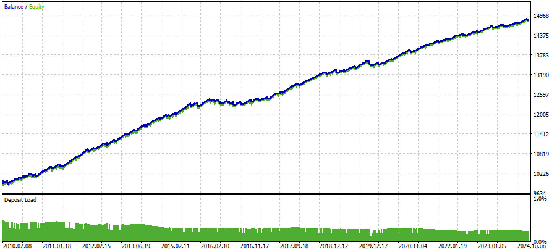
Fig. 3. Testing the trained model using the mean reversion strategy

Conclusion

This article demonstrates all the steps involved in developing a mean reversion strategy using machine learning. It outlines a comprehensive approach: from trade labeling and market regime identification to model training and the creation of a fully-fledged trading bot.

The article includes all the necessary codes for independent experiments.

Python files.zip contains the following files for development in the Python environment:

Filename	Description
mean reversion.py	The main script for training models
labeling_lib.py	Module with deal markers
tester_lib.py	Custom strategy tester based on machine learning
export_lib.py	The library for exporting models to the MetaTrader 5 terminal in ONNX format
EURGBP_H1.csv	The file with quotes exported from the MetaTrader 5 terminal

MQL5 files.zip contains files for the MetaTrader 5 terminal:

Filename	Description
mean reversion.ex5	The compiled bot from the article
mean reversion.mq5	Bot source code from the article
folder Include//Mean reversion	The ONNX models and the header file for connecting to the bot