Circle Search Algorithm (CSA)

Contents

1. Introduction
2. Implementation of the algorithm
3. Test results

Introduction

Circle Search Algorithm (CSA) is a new optimization method inspired by the geometric properties of a circle. Its uniqueness lies in the use of trigonometric relationships and geometric principles to explore the search space.

The CSA is based on an interesting idea where each search point moves along a trajectory defined by a tangent to a circle, which creates a balance between global exploration and local refinement of the solution. This approach is original because a circle has unique mathematical properties — a constant radius and a continuous derivative — which ensures smooth movement of agents in the search space.

The algorithm combines two phases: exploitation and exploration. In the exploitation phase, agents focus on promising areas, moving more directionally, while in the exploration phase they make bolder leaps into unexplored areas of the solution space. The transition between phases is regulated by a mechanism based on the current iteration and a special "c" parameter.

What makes CSA particularly attractive is its ability to work efficiently in high-dimensional spaces while maintaining an intuitive geometric interpretation. Each agent in the population follows its own unique trajectory, determined by the θ angle, which is dynamically adjusted during the search.

Circle Search Algorithm (CSA) was developed by researchers Mohammad H. Kaiys, Hany M. Hasanien and others and was published in 2022.

Implementation of the algorithm

The Circle Search Algorithm (CSA) aims to find the optimal solution in random circles in order to expand the search area. It uses the center of the circle as a target point. The process begins with the angle between the tangent and the circle gradually decreasing, allowing the tangent to approach the center (Figure 1).

To provide variety in the search and avoid getting stuck in local optima, the angle of tangential contact also changes randomly. In the context of the algorithm, the Xt tangent point acts as a search agent, while the Xc central point denotes the best solution found.

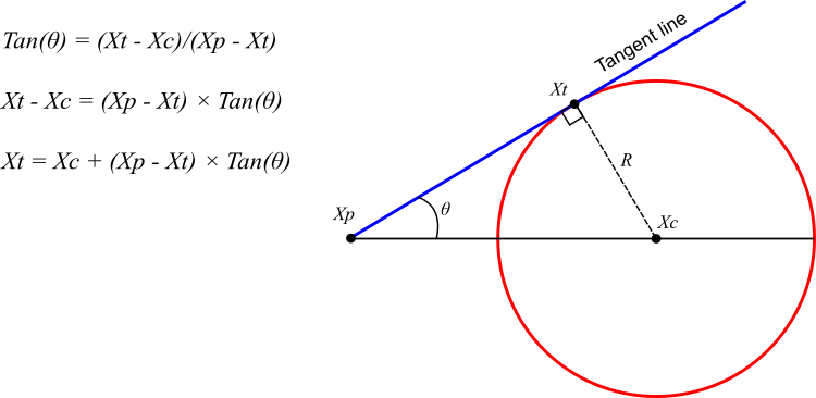
Figure 1. Geometric properties of a circle and its tangent

CSA adapts the position of the search agent in response to the movement of the touch point towards the center. This allows for improving the quality of the solution, while randomly updating the tangential contact angle serves as an important mechanism for avoiding local minima. The main stages of the CSA optimizer operation are displayed in the diagram below.

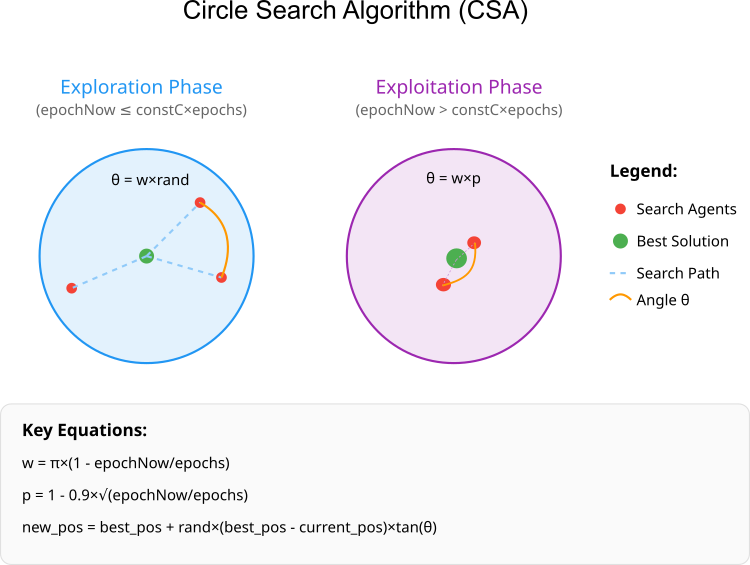
Figure 2. CSA operation chart

Next, an angle is determined for each agent. If the current iteration is greater than the product of the threshold and the maximum number of iterations, the agent is in the exploration phase, otherwise the exploitation phase is applied (see Figure 2). Agent positions are updated and the suitability of each one is assessed. The results are compared with the current best solution, and if a better one is found, the position is updated. An iteration is terminated by incrementing the iteration counter. When the algorithm completes its execution, it returns the best position found and its fitness value.

The algorithm uses the concept of moving points along a tangent to a circle, where each search agent moves at a certain θ angle relative to the current best solution. This movement is governed by several parameters (w, a, p) that change over time. As noted above, the algorithm operation is divided into two phases: exploration, when agents make wider movements to find promising areas, and exploitation, when agents focus on refining the solutions found.

The final version I proposed contains several differences that significantly improve the algorithm search capabilities. Changed the w update equation:

• The original one: w = w × rand - w
• The final code: w = π × (1 - epochNow/epochs) This made the change of the w parameter more predictable and linear, which improves the convergence of the algorithm.

Modified the position update equation:

• The original one: Xi = Xc + (Xc - Xi) × tan(θ)
• The final version: Xi = Xc + rand × (Xc - Xi) × tan(θ) Adding a random factor "rand [0.0; 1.0]" adds extra stochasticity to the search and improves it over the original version. 

Optimized the update phase:

• Added local best solution update for each agent
• Improved balancing strategy between global and local search

The main conceptual difference is that the final version made the algorithm more "smooth" and predictable in its behavior, while maintaining the ability to search. The original algorithm was more "chaotic" in its behavior, while the final version provides a more controlled optimization, especially in terms of the transition between the exploration and exploitation phases.

Now we can start developing the pseudocode for the algorithm.

Circle Search Algorithm (CSA) pseudocode:

1. Initialization:
   • Set population size (popSize = 50)
   • Set the phase constant of the study (constC = 0.8)
   • Initialize initial parameters:
     • w = π (angle parameter)
     • a = π
       
     • p = 1.0
       
     • θ = 0 (initial angle)
2. In case of the first iteration (revision = false):
   • For each i agent in the population:
     • Randomly initialize coordinates within the given boundaries
     • Adjust coordinates according to the change step
   • Set revision = true
   • Return to the start
3. Otherwise (main optimization loop):
   • Increase the iteration counter (epochNow++)
   • Update parameters:
     • w = π × (1 - epochNow/epochs) // linear decrease
     • a = π - π × (epochNow/epochs)²
     • p = 1 - 0.9 × √(epochNow/epochs)
4. For each agent in the population:
   • Determine the current phase:
     • If epochNow ≤ constC × epochs: → Exploration phase: θ = w × random [0.0; 1.0]
     • Otherwise: → Exploitation phase: θ = w × p
   • Update the agent position:
     • For each coordinate j: → new_pos = best_pos + random [0.0; 1.0] × (best_pos - current_pos) × tan (θ) → Adjust new_pos within the given limits
5. Revision of results:
   • For each agent:
     • If agent fitness > global best fitness: → Update global best solution
     • If agent fitness > best local fitness: → Update agent's local best solution
6. Repeat steps 3-5 until the stopping criterion is reached
   

Let's move on to implementation. The C_AO_CSA class is an implementation of the CSA algorithm and is inherited from the C_AO base class. Let's look at its main elements and structure:

Constructor initializes the algorithm parameters. It specifies the name and description of the algorithm, and sets values for the parameters:

• popSize — population size equal to 50.
• constC — constant equal to 0.8 used in the exploration phase.
• w, aParam, p, theta — initial values of the parameters to be used in the algorithm.

Methods:

• SetParams () — method for setting parameter values based on the "params" data array.
• Init () — the method is implemented to initialize the parameters related to the ranges of values and the number of epochs, over which the algorithm will be executed.
• Moving () — used to move particles and perform algorithm iterations.
• Revision () — to analyze and adjust the state of the population.

Private methods:

• CalculateW (), CalculateA (), CalculateP (), CalculateTheta () — methods for calculating the corresponding parameters.
• IsExplorationPhase () — method determines whether the algorithm is in the exploration phase.

//——————————————————————————————————————————————————————————————————————————————
class C_AO_CSA : public C_AO
{
  public: //--------------------------------------------------------------------
  C_AO_CSA ()
  {
    ao_name = "CSA";
    ao_desc = "Circle Search Algorithm";
    ao_link = "https://www.mql5.com/en/articles/17143";

    popSize = 50;     // population size
    constC  = 0.8;    // optimal value for the exploration phase
    w       = M_PI;   // initial value w
    aParam  = M_PI;   // initial value a
    p       = 1.0;    // initial value p
    theta   = 0;      // initial value of the angle

    ArrayResize (params, 2);
    params [0].name = "popSize";     params [0].val = popSize;
    params [1].name = "constC";      params [1].val = constC;
  }

  void SetParams ()
  {
    popSize = (int)params [0].val;
    constC  = params      [1].val;
  }

  bool Init (const double &rangeMinP  [],  // minimum values
             const double &rangeMaxP  [],  // maximum values
             const double &rangeStepP [],  // step change
             const int     epochsP = 0);   // number of epochs

  void Moving   ();
  void Revision ();

  //----------------------------------------------------------------------------
  double constC;      // constant for determining the search phase [0,1]

  private: //-------------------------------------------------------------------
  int epochs;         // maximum number of iterations
  int epochNow;       // current iteration

  // Parameters for CSA
  double w;           // parameter for calculating the angle
  double aParam;      // parameter a from the equation (8)
  double p;           // parameter p from the equation (9)
  double theta;       // search angle

  double CalculateW ();
  double CalculateA ();
  double CalculateP ();
  double CalculateTheta (double currentW, double currentP);
  bool IsExplorationPhase ();
};
//——————————————————————————————————————————————————————————————————————————————

The Init method is intended to initialize the parameters of the CSA algorithm. Its parameters include the rangeMinP[] array of minimum values of the search space, the rangeMaxP[] array of maximum values, the rangeStepP[] array of changing values increments, and the number of epochs specified by the epochsP parameter, which defaults to 0.

During the execution of the method, StandardInit is called, the purpose of which is to attempt to initialize the standard parameters. If initialization is successful, the values for the epochs and epochNow variables are set. The epochs variable gets its value from epochsP, while epochNow is cleared. The method completes execution by returning 'true', which indicates successful initialization of the algorithm parameters.

//——————————————————————————————————————————————————————————————————————————————
bool C_AO_CSA::Init (const double &rangeMinP  [],
                     const double &rangeMaxP  [],
                     const double &rangeStepP [],
                     const int     epochsP = 0)
{
  if (!StandardInit (rangeMinP, rangeMaxP, rangeStepP)) return false;

  //----------------------------------------------------------------------------
  epochs   = epochsP;
  epochNow = 0;
  return true;
}
//——————————————————————————————————————————————————————————————————————————————

The Moving method in the C_AO_CSA class implements the logic for updating agent positions within the CSA algorithm. At the beginning of the method, the current epoch counter is incremented, which allows us to track how many iterations have been performed (used in calculation equations). Then a check is performed to determine whether the agents' coordinates need to be initialized. If this is the first method execution, random coordinates are generated for all agents in the given ranges. These coordinates are then adapted to take into account the given steps. After this, the flag about the need for revision is set to true.

If the method is not called for the first time, then the key parameters of the algorithm, such as w, aParam and p, are updated. Then, for each agent, the theta angle is calculated and used to update its coordinates. Each coordinate is updated taking into account the coordinates of the best agent, the influence of the random factor and the theta angle. After this, the results are also adjusted to stay within the specified ranges.

//——————————————————————————————————————————————————————————————————————————————
void C_AO_CSA::Moving ()
{
  epochNow++;

  //----------------------------------------------------------------------------
  if (!revision)
  {
    for (int i = 0; i < popSize; i++)
    {
      for (int j = 0; j < coords; j++)
      {
        a [i].c [j] = u.RNDfromCI (rangeMin [j], rangeMax [j]);
        a [i].c [j] = u.SeInDiSp (a [i].c [j], rangeMin [j], rangeMax [j], rangeStep [j]);
      }
    }
    revision = true;
    return;
  }

  //----------------------------------------------------------------------------
  w      = CalculateW ();    // Update w linearly
  aParam = CalculateA ();    // Update a
  p      = CalculateP ();    // Update p

  for (int i = 0; i < popSize; i++)
  {
    theta = CalculateTheta (w, p);

    for (int j = 0; j < coords; j++)
    {
      a [i].c [j] = cB [j] + u.RNDprobab () * (cB [j] - a [i].c  [j]) * tan (theta);
      a [i].c [j] = u.SeInDiSp (a [i].c [j], rangeMin [j], rangeMax [j], rangeStep [j]);
    }
  }
}
//——————————————————————————————————————————————————————————————————————————————

The Revision method is responsible for updating the best solutions across the entire population. It checks the current values of the agents' objective function and updates the corresponding parameters if better solutions are found.

//——————————————————————————————————————————————————————————————————————————————
void C_AO_CSA::Revision ()
{
  for (int i = 0; i < popSize; i++)
  {
    // Update the best global solution
    if (a [i].f > fB)
    {
      fB = a [i].f;
      ArrayCopy (cB, a [i].c, 0, 0, WHOLE_ARRAY);
    }
  }
}
//——————————————————————————————————————————————————————————————————————————————

The CalculateW method is designed to calculate the value of the w parameter, which decreases linearly from the initial value (M_PI) to "0" with an increase in the number of current epochs (epochNow) relative to the total number of epochs and returns the calculated value of w. This calculated parameter is involved in the equation for calculating the Theta angle.

//——————————————————————————————————————————————————————————————————————————————
double C_AO_CSA::CalculateW ()
{
  // Linear decrease of w from the initial value (M_PI) to 0
  return M_PI * (1.0 - (double)epochNow / epochs);
  //return w * u.RNDprobab () - w;
}
//——————————————————————————————————————————————————————————————————————————————

The CalculateA method calculates the aParam value that decreases from M_PI to 0 as epochNow increases, quadratically depending on the total number of epochs.

//——————————————————————————————————————————————————————————————————————————————
double C_AO_CSA::CalculateA ()
{
  return M_PI - M_PI * MathPow ((double)epochNow / epochs, 2);
}
//——————————————————————————————————————————————————————————————————————————————

The CalculateP method calculates the p value that decreases from "1.0" to "0.1" as epochNow increases, i.e., it depends on the current epoch.

//——————————————————————————————————————————————————————————————————————————————
double C_AO_CSA::CalculateP ()
{
  return 1.0 - 0.9 * MathPow ((double)epochNow / epochs, 0.5);
}
//——————————————————————————————————————————————————————————————————————————————

The CalculateTheta method calculates the value of Theta using the current currentW and currentP parameters.

• If the current phase is research, return currentW multiplied by a random number.
• Otherwise, return the product of currentW and currentP.

//——————————————————————————————————————————————————————————————————————————————
double C_AO_CSA::CalculateTheta (double currentW, double currentP)
{
  // Use the aParam parameter to adjust the angle
  if (IsExplorationPhase ()) return currentW * u.RNDprobab ();
  else return currentW * currentP;

}
//——————————————————————————————————————————————————————————————————————————————

The IsExplorationPhase method checks whether the current iteration is in the exploration phase.

//——————————————————————————————————————————————————————————————————————————————
bool C_AO_CSA::IsExplorationPhase ()
{
  // Research in the first part of the iterations (constC is usually 0.8)
  return (epochNow <= constC * epochs);
}
//——————————————————————————————————————————————————————————————————————————————

Test results

The algorithm's authors position it as a highly efficient optimization method. However, after implementation, some improvements, and final testing, the results are not very impressive. The algorithm was able to enter the ranking table, but its performance is significantly inferior to the best algorithmic solutions at the moment.

CSA|Circle Search Algorithm|50.0|0.8|
=============================
5 Hilly's; Func runs: 10000; result: 0.6656012653478078
25 Hilly's; Func runs: 10000; result: 0.4531682514562617
500 Hilly's; Func runs: 10000; result: 0.2912586479936386
=============================
5 Forest's; Func runs: 10000; result: 0.6879687203647712
25 Forest's; Func runs: 10000; result: 0.41397289345600924
500 Forest's; Func runs: 10000; result: 0.2052507546137296
=============================
5 Megacity's; Func runs: 10000; result: 0.3753846153846153
25 Megacity's; Func runs: 10000; result: 0.2363076923076922
500 Megacity's; Func runs: 10000; result: 0.10646153846153927
=============================
All score: 3.43537 (38.17%)

The visualization of the algorithm operation shows problems with convergence and getting stuck at local extremes. Nevertheless, the algorithm tries to work to the best of its ability. Despite the problems with getting stuck in traps (this is clearly visible from the long horizontal sections in the convergence graph), one can highlight its ability to work quite effectively on high-dimensional problems.

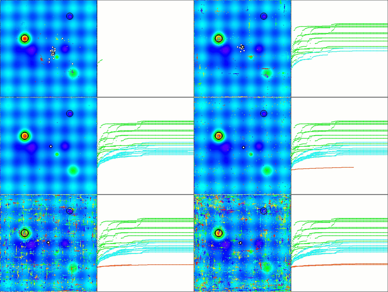
CSA on the Hilly test function

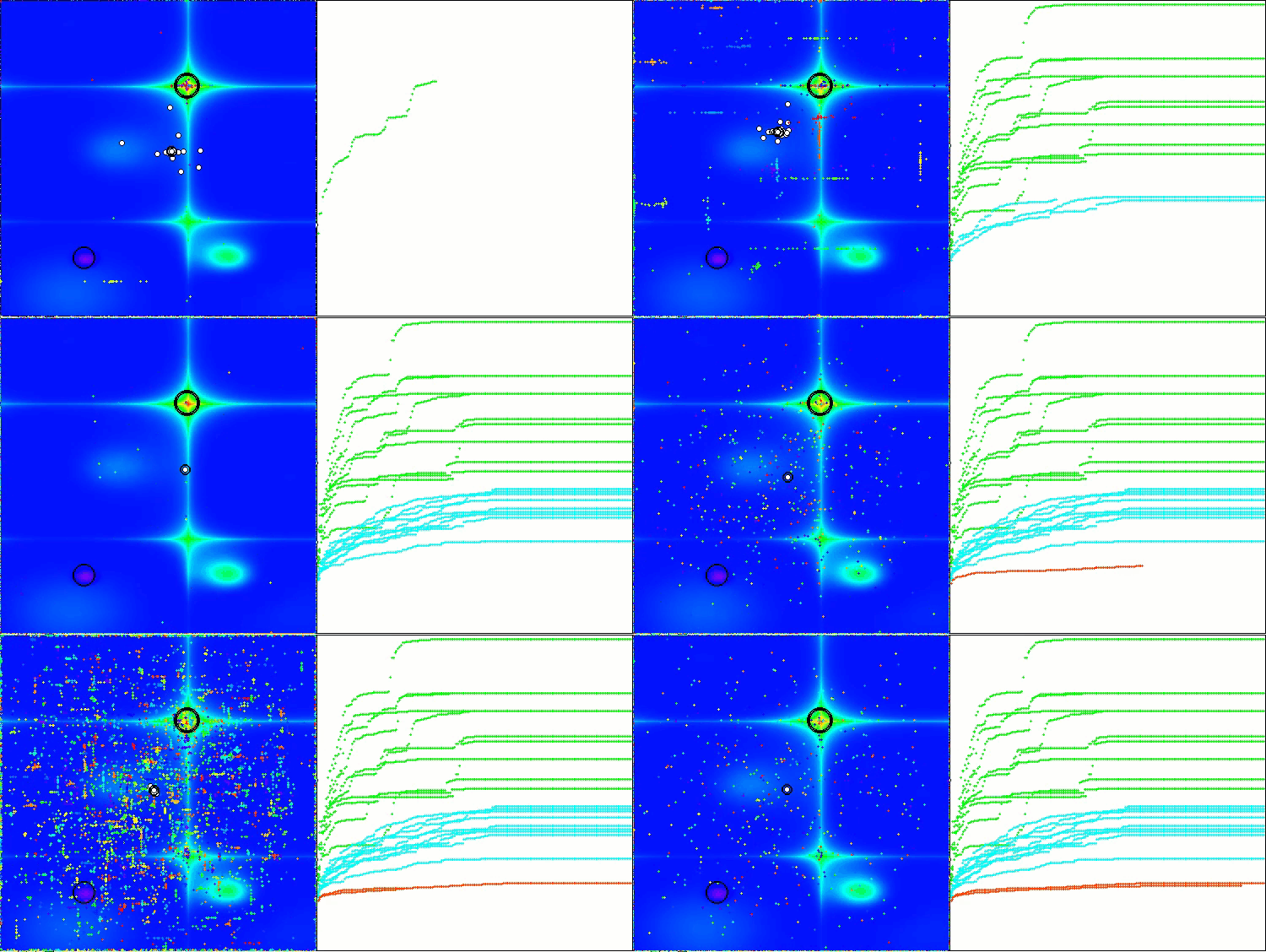
CSA on the Forest test function

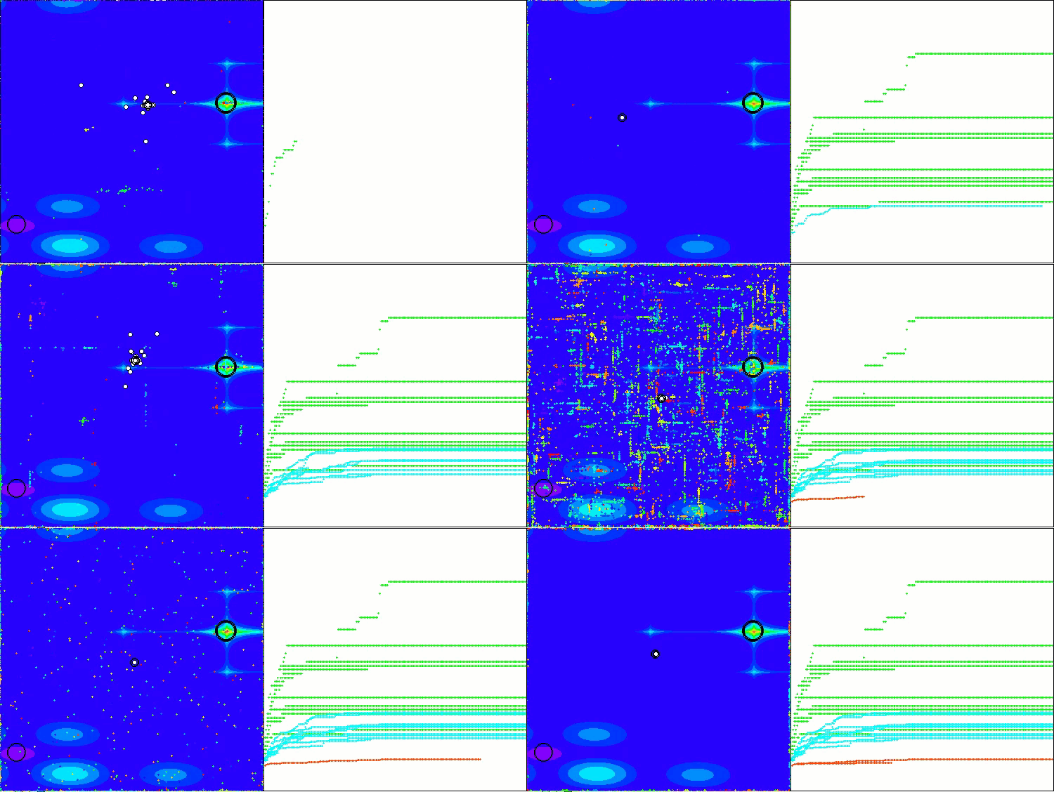
CSA on the Megacity test function

Based on the results of the algorithm testing, CSA ranks 41st in the ranking table.

#	AO	Description	Hilly			Hilly final	Forest			Forest final	Megacity (discrete)			Megacity final	Final result	% of MAX
			10 p (5 F)	50 p (25 F)	1000 p (500 F)		10 p (5 F)	50 p (25 F)	1000 p (500 F)		10 p (5 F)	50 p (25 F)	1000 p (500 F)
1	ANS	across neighbourhood search	0.94948	0.84776	0.43857	2.23581	1.00000	0.92334	0.39988	2.32323	0.70923	0.63477	0.23091	1.57491	6.134	68.15
2	CLA	code lock algorithm (joo)	0.95345	0.87107	0.37590	2.20042	0.98942	0.91709	0.31642	2.22294	0.79692	0.69385	0.19303	1.68380	6.107	67.86
3	AMOm	animal migration ptimization M	0.90358	0.84317	0.46284	2.20959	0.99001	0.92436	0.46598	2.38034	0.56769	0.59132	0.23773	1.39675	5.987	66.52
4	(P+O)ES	(P+O) evolution strategies	0.92256	0.88101	0.40021	2.20379	0.97750	0.87490	0.31945	2.17185	0.67385	0.62985	0.18634	1.49003	5.866	65.17
5	CTA	comet tail algorithm (joo)	0.95346	0.86319	0.27770	2.09435	0.99794	0.85740	0.33949	2.19484	0.88769	0.56431	0.10512	1.55712	5.846	64.96
6	TETA	time evolution travel algorithm (joo)	0.91362	0.82349	0.31990	2.05701	0.97096	0.89532	0.29324	2.15952	0.73462	0.68569	0.16021	1.58052	5.797	64.41
7	SDSm	stochastic diffusion search M	0.93066	0.85445	0.39476	2.17988	0.99983	0.89244	0.19619	2.08846	0.72333	0.61100	0.10670	1.44103	5.709	63.44
8	AAm	archery algorithm M	0.91744	0.70876	0.42160	2.04780	0.92527	0.75802	0.35328	2.03657	0.67385	0.55200	0.23738	1.46323	5.548	61.64
9	ESG	evolution of social groups (joo)	0.99906	0.79654	0.35056	2.14616	1.00000	0.82863	0.13102	1.95965	0.82333	0.55300	0.04725	1.42358	5.529	61.44
10	SIA	simulated isotropic annealing (joo)	0.95784	0.84264	0.41465	2.21513	0.98239	0.79586	0.20507	1.98332	0.68667	0.49300	0.09053	1.27020	5.469	60.76
11	ACS	artificial cooperative search	0.75547	0.74744	0.30407	1.80698	1.00000	0.88861	0.22413	2.11274	0.69077	0.48185	0.13322	1.30583	5.226	58.06
12	DA	dialectical algorithm	0.86183	0.70033	0.33724	1.89940	0.98163	0.72772	0.28718	1.99653	0.70308	0.45292	0.16367	1.31967	5.216	57.95
13	BHAm	black hole algorithm M	0.75236	0.76675	0.34583	1.86493	0.93593	0.80152	0.27177	2.00923	0.65077	0.51646	0.15472	1.32195	5.196	57.73
14	ASO	anarchy society optimization	0.84872	0.74646	0.31465	1.90983	0.96148	0.79150	0.23803	1.99101	0.57077	0.54062	0.16614	1.27752	5.178	57.54
15	RFO	royal flush optimization (joo)	0.83361	0.73742	0.34629	1.91733	0.89424	0.73824	0.24098	1.87346	0.63154	0.50292	0.16421	1.29867	5.089	56.55
16	AOSm	atomic orbital search M	0.80232	0.70449	0.31021	1.81702	0.85660	0.69451	0.21996	1.77107	0.74615	0.52862	0.14358	1.41835	5.006	55.63
17	TSEA	turtle shell evolution algorithm (joo)	0.96798	0.64480	0.29672	1.90949	0.99449	0.61981	0.22708	1.84139	0.69077	0.42646	0.13598	1.25322	5.004	55.60
18	DE	differential evolution	0.95044	0.61674	0.30308	1.87026	0.95317	0.78896	0.16652	1.90865	0.78667	0.36033	0.02953	1.17653	4.955	55.06
19	CRO	chemical reaction optimization	0.94629	0.66112	0.29853	1.90593	0.87906	0.58422	0.21146	1.67473	0.75846	0.42646	0.12686	1.31178	4.892	54.36
20	BSA	bird swarm algorithm	0.89306	0.64900	0.26250	1.80455	0.92420	0.71121	0.24939	1.88479	0.69385	0.32615	0.10012	1.12012	4.809	53.44
21	HS	harmony search	0.86509	0.68782	0.32527	1.87818	0.99999	0.68002	0.09590	1.77592	0.62000	0.42267	0.05458	1.09725	4.751	52.79
22	SSG	saplings sowing and growing	0.77839	0.64925	0.39543	1.82308	0.85973	0.62467	0.17429	1.65869	0.64667	0.44133	0.10598	1.19398	4.676	51.95
23	BCOm	bacterial chemotaxis optimization M	0.75953	0.62268	0.31483	1.69704	0.89378	0.61339	0.22542	1.73259	0.65385	0.42092	0.14435	1.21912	4.649	51.65
24	ABO	african buffalo optimization	0.83337	0.62247	0.29964	1.75548	0.92170	0.58618	0.19723	1.70511	0.61000	0.43154	0.13225	1.17378	4.634	51.49
25	(PO)ES	(PO) evolution strategies	0.79025	0.62647	0.42935	1.84606	0.87616	0.60943	0.19591	1.68151	0.59000	0.37933	0.11322	1.08255	4.610	51.22
26	TSm	tabu search M	0.87795	0.61431	0.29104	1.78330	0.92885	0.51844	0.19054	1.63783	0.61077	0.38215	0.12157	1.11449	4.536	50.40
27	BSO	brain storm optimization	0.93736	0.57616	0.29688	1.81041	0.93131	0.55866	0.23537	1.72534	0.55231	0.29077	0.11914	0.96222	4.498	49.98
28	WOAm	wale optimization algorithm M	0.84521	0.56298	0.26263	1.67081	0.93100	0.52278	0.16365	1.61743	0.66308	0.41138	0.11357	1.18803	4.476	49.74
29	AEFA	artificial electric field algorithm	0.87700	0.61753	0.25235	1.74688	0.92729	0.72698	0.18064	1.83490	0.66615	0.11631	0.09508	0.87754	4.459	49.55
30	AEO	artificial ecosystem-based optimization algorithm	0.91380	0.46713	0.26470	1.64563	0.90223	0.43705	0.21400	1.55327	0.66154	0.30800	0.28563	1.25517	4.454	49.49
31	ACOm	ant colony optimization M	0.88190	0.66127	0.30377	1.84693	0.85873	0.58680	0.15051	1.59604	0.59667	0.37333	0.02472	0.99472	4.438	49.31
32	BFO-GA	bacterial foraging optimization - ga	0.89150	0.55111	0.31529	1.75790	0.96982	0.39612	0.06305	1.42899	0.72667	0.27500	0.03525	1.03692	4.224	46.93
33	SOA	simple optimization algorithm	0.91520	0.46976	0.27089	1.65585	0.89675	0.37401	0.16984	1.44060	0.69538	0.28031	0.10852	1.08422	4.181	46.45
34	ABHA	artificial bee hive algorithm	0.84131	0.54227	0.26304	1.64663	0.87858	0.47779	0.17181	1.52818	0.50923	0.33877	0.10397	0.95197	4.127	45.85
35	ACMO	atmospheric cloud model optimization	0.90321	0.48546	0.30403	1.69270	0.80268	0.37857	0.19178	1.37303	0.62308	0.24400	0.10795	0.97503	4.041	44.90
36	ADAMm	adaptive moment estimation M	0.88635	0.44766	0.26613	1.60014	0.84497	0.38493	0.16889	1.39880	0.66154	0.27046	0.10594	1.03794	4.037	44.85
37	ATAm	artificial tribe algorithm M	0.71771	0.55304	0.25235	1.52310	0.82491	0.55904	0.20473	1.58867	0.44000	0.18615	0.09411	0.72026	3.832	42.58
38	ASHA	artificial showering algorithm	0.89686	0.40433	0.25617	1.55737	0.80360	0.35526	0.19160	1.35046	0.47692	0.18123	0.09774	0.75589	3.664	40.71
39	ASBO	adaptive social behavior optimization	0.76331	0.49253	0.32619	1.58202	0.79546	0.40035	0.26097	1.45677	0.26462	0.17169	0.18200	0.61831	3.657	40.63
40	MEC	mind evolutionary computation	0.69533	0.53376	0.32661	1.55569	0.72464	0.33036	0.07198	1.12698	0.52500	0.22000	0.04198	0.78698	3.470	38.55
41	CSA	circle search algorithm	0.66560	0.45317	0.29126	1.41003	0.68797	0.41397	0.20525	1.30719	0.37538	0.23631	0.10646	0.71815	3.435	38.17
42	IWO	invasive weed optimization	0.72679	0.52256	0.33123	1.58058	0.70756	0.33955	0.07484	1.12196	0.42333	0.23067	0.04617	0.70017	3.403	37.81
43	Micro-AIS	micro artificial immune system	0.79547	0.51922	0.30861	1.62330	0.72956	0.36879	0.09398	1.19233	0.37667	0.15867	0.02802	0.56335	3.379	37.54
44	COAm	cuckoo optimization algorithm M	0.75820	0.48652	0.31369	1.55841	0.74054	0.28051	0.05599	1.07704	0.50500	0.17467	0.03380	0.71347	3.349	37.21
45	SDOm	spiral dynamics optimization M	0.74601	0.44623	0.29687	1.48912	0.70204	0.34678	0.10944	1.15826	0.42833	0.16767	0.03663	0.63263	3.280	36.44
	RW	random walk	0.48754	0.32159	0.25781	1.06694	0.37554	0.21944	0.15877	0.75375	0.27969	0.14917	0.09847	0.52734	2.348	26.09

Summary

Based on the results of testing and analyzing the performance of the Circle Search Algorithm (CSA), the following conclusions can be drawn: despite the elegance of the geometric concept and the intuitive search mechanism based on movement along tangents to a circle, the algorithm demonstrates relatively weak results in comparative analysis, occupying 41st place out of 45 in the optimization algorithms rating table. This situation indicates significant limitations in its current implementation.

The main problems of the algorithm are related to its tendency to get stuck in local extrema, which is especially noticeable when working on simple problems of small dimension. This may be due to several factors: firstly, the corner search mechanism, although it seems promising, in practice turns out to be insufficient in overcoming local optima. Secondly, the balance between the exploration and exploitation phases, regulated by the constC parameter, does not provide sufficient diversification of the search. The entire population collapses to pseudo-good solutions, that is, to a single point, and even attempts to "shake" the population with a random component in the main equation for updating the position of agents in the solution space did not help.

An attempt to improve the algorithm by adding a random multiplier to the equation for updating the agents' positions, although it led to more predictable behavior of the algorithm, failed to significantly increase its efficiency. This may indicate that the basic idea of the algorithm, based on the geometric properties of a circle, is either not fully realized by the authors in the current implementation, or has fundamental limitations in the context of global optimization.

However, the algorithm demonstrates certain search capabilities and may be effective for some specific problems, especially those where the objective function landscape is relatively simple. To improve the efficiency of the algorithm, I can recommend further research in the direction of improving the mechanism for exiting local optima, possibly by introducing additional mechanisms for search diversification or hybridization with other optimization methods (as a priority, the use of this search strategy in other optimization algorithms as a component).

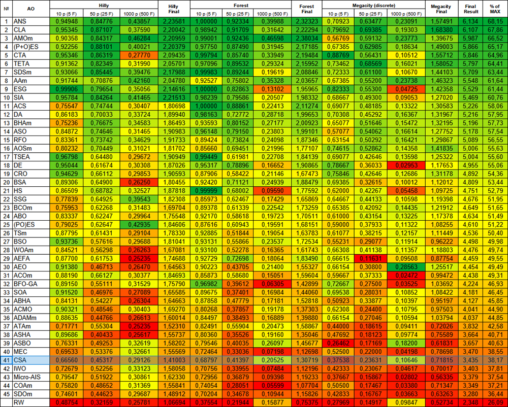
Figure 3. Color gradation of algorithms according to the corresponding tests

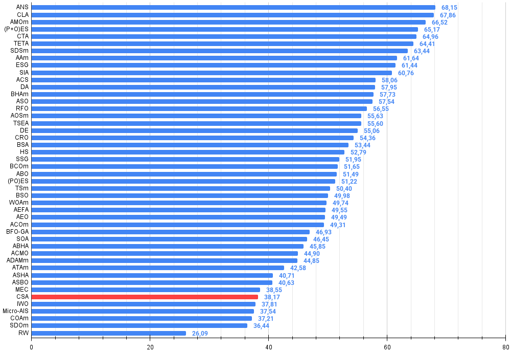
Figure 4. Histogram of algorithm testing results (scale from 0 to 100, the higher the better, where 100 is the maximum possible theoretical result, in the archive there is a script for calculating the rating table)

CSA pros and cons:

Pros:

1. Very few external parameters
   
2. Simple implementation
3. An interesting idea using the geometric properties of a circle
   

Disadvantages:

1. Low convergence accuracy
   
2. Gets stuck in local extremes

The article is accompanied by an archive with the current versions of the algorithm codes. The author of the article is not responsible for the absolute accuracy in the description of canonical algorithms. Changes have been made to many of them to improve search capabilities. The conclusions and judgments presented in the articles are based on the results of the experiments.

• github: https://github.com/JQSakaJoo/Population-optimization-algorithms-MQL5

Programs used in the article

#	Name	Type	Description
1	#C_AO.mqh	Include	Parent class of population optimization algorithms
2	#C_AO_enum.mqh	Include	Enumeration of population optimization algorithms
3	TestFunctions.mqh	Include	Library of test functions
4	TestStandFunctions.mqh	Include	Test stand function library
5	Utilities.mqh	Include	Library of auxiliary functions
6	CalculationTestResults.mqh	Include	Script for calculating results in the comparison table
7	Testing AOs.mq5	Script	The unified test stand for all population optimization algorithms
8	Simple use of population optimization algorithms.mq5	Script	A simple example of using population optimization algorithms without visualization
9	Test_AO_CSA.mq5	Script	CSA test stand