
Neural Networks in Trading: Two-Dimensional Connection Space Models (Chimera)

Introduction
Time series modeling represents a complex task with broad applications across various domains, including medicine, financial markets, and energy systems. The main challenges in developing universal time series models are associated with:
- Accounting for multi-scale dependencies, including short-term autocorrelations, seasonality, and long-term trends. This requires the use of flexible and powerful architectures.
- Adaptive handling of multivariate time series, where relationships between variables can be dynamic and nonlinear. This requires mechanisms that considers context-dependent interactions.
- Minimizing the need for manual data preprocessing, ensuring automatic identification of structural patterns without extensive parameter tuning.
- Computational efficiency, especially when processing long sequences, which requires model architecture optimization for efficient use of computational resources and reduced training costs.
Classical statistical methods require significant preprocessing of raw data and often fail to adequately capture complex nonlinear dependencies. Deep neural network architectures have demonstrated high expressiveness, but the quadratic computational complexity of Transformer-based models makes them difficult to apply to multivariate time series with a large number of features. Furthermore, such models often fail to distinguish seasonal and long-term components or rely on rigid a priori assumptions, limiting their adaptability in various practical scenarios.
One approach addressing these issues was proposed in the paper "Chimera: Effectively Modeling Multivariate Time Series with 2-Dimensional State Space Models". The Chimera framework is a two-dimensional state space model (2D-SSM) that applies linear transformations both along the temporal axis and along the variable axis. Chimera comprises three primary components: state space models along the time dimension, along the variables dimension, and cross-dimensional transitions. Its parameterization is based on compact diagonal matrices, enabling it to replicate both classical statistical methods and modern SSM architectures.
Additionally, Chimera incorporates adaptive discretization to account for seasonal patterns and characteristics of dynamic systems.
The authors of Chimera evaluated the framework performance across various multivariate time series tasks, including classification, forecasting, and anomaly detection. Experimental results demonstrate that Chimera achieves accuracy comparable to, or exceeding, state-of-the-art methods while reducing overall computational costs.
The Chimera Algorithm
State space models (SSMs) play an important role in time series analysis due to their simplicity and expressive power in modeling complex dependencies, including autoregressive relationships. These models represent systems in which the current state depends on the previous state of the observed environment. Traditionally, however, SSMs describe systems where the state depends on a single variable (e.g., time). This limits their applicability to multivariate time series, where dependencies must be captured both temporally and across variables.
Multivariate time series are inherently more complex, requiring methods capable of modeling interdependencies between multiple variables simultaneously. Classical two-dimensional state space models (2D-SSMs) used for such tasks face several limitations compared to modern deep learning methods. The following can be highlighted here:
- Restriction to linear dependencies. Traditional 2D-SSMs can only model linear relationships, which limits their ability to represent the complex, nonlinear dependencies characteristic of real multivariate time series.
- Discrete model resolution. These models often have predefined resolutions and cannot automatically adapt to changes in data characteristics, reducing their effectiveness for modeling seasonal or variable-resolution patterns.
- Difficulty with large datasets. In practice, 2D-SSMs are often inefficient for handling large volumes of data, limiting their practical utility.
- Static parameter updates. Classical update mechanisms are fixed, failing to account for dynamic dependencies that evolve over time. This is a significant limitation in applications where data evolve and require adaptive approaches.
In contrast, deep learning methods, which have developed rapidly in recent years, offer the potential to overcome many of these limitations. They enable modeling of complex nonlinear dependencies and temporal dynamics, making them promising for multivariate time series analysis.
In Chimera, 2D-SSMs are used to model multivariate time series, where the first axis corresponds to time, and the second axis corresponds to variables. Each state depends on both time and variables. The first step is to transform the continuous 2D-SSM into a discrete form, considering step sizes Δ1 and Δ2, representing the signal resolution along each axis. Using the Zero-Order Hold (ZOH) method, the original data can be discretized as:
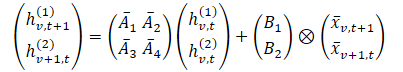
where t and v indicate indices along the temporal and variable dimensions, respectively. This expression can be represented in a simpler form.
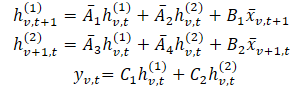
In this formulation: hv,t(1) — is a hidden state carrying temporal information (each state depends on the previous time step for the same variable), with A1 and A2 controlling the emphasis on past cross-time and cross-variable information, respectively. Then hv,t(2) is a hidden state carrying cross-variable information (each state depends on other variables at the same time step).
Time series data are often sampled from an underlying continuous process. In such cases, Δ1 can be interpreted as the temporal resolution or sampling frequency. Discretization along the variable axis, which is inherently discrete, is less intuitive but essential. In 1D-SSMs, discretization is closely linked to RNN gate mechanisms, providing model normalization and desired properties like resolution invariance.
A 2D discrete SSM with parameters ({Ai}, {Bi}, {Ci}, kΔ1, ℓΔ2) evolves k times faster along time than a 2D discrete SSM with parameters ({Ai}, {Bi}, {Ci}, Δ1ℓΔ2), and ℓ times faster ({Ai}, {Bi}, {Ci}, kΔ1, Δ2). Hence, Δ1 can me thorught of as a controller of the dependency length captured by the model. Based on the above description, we see discretization along the time axis as setting the resolution or sampling frequency. Smaller Δ1 captures long-term progression, while larger Δ1 captures seasonal patterns.
Discretization along the variable axis is analogous to RNN gates, where Δ2 controls the model's context length. Larger Δ2 values result in smaller context windows, reducing variable interactions, while smaller Δ2 values emphasize inter-variable dependencies.
To enhance expressiveness and enable autoregressive recovery, hidden states hv,t(1) carry past temporal information. The authors restrict matrices A1 and A2, to structured forms. And even simple diagonal matrices for A3 and A4 effectively merge cross-variable information.
Because 2D-SSMs are causal along the variable dimension (which lacks intrinsic order), Chimera uses separate forward and backward modules along the feature dimension to address information flow limitations.
Similar to effective 1D-SSMs, a data-independent formulation can be interpreted as a convolution with kernel K. This enables faster training through parallelization and connects Chimera with recent convolution-based architectures for time series.
As discussed earlier, parametersA1 and A2 control the emphasis on past cross-temporal and cross-variation information. Similarly, Δ1 and B1 govern emphasis on current and historical input. These data-independent parameters represent global system features. But in complex systems, emphasis depends on the current input. Therefore, it is necessary that these parameters be a function of the original data. The analyzed parameter dependency provides a mechanism analogous to Transformers for adaptive selection of relevant and filtering of irrelevant information for each input set. In addition, depending on the data, the model should adaptively learn to mix information across variations. Making the parameters dependent on the input data further addresses this issue and allows the model to mix relevant and filter out irrelevant parameters to model the variable of interest. One of the technical contributions of Chimera is the construction of Bi, Ci and Δi by a function of input 𝐱v,t.
Chimera stacks 2D-SSMs with nonlinearities between layers. To enhance the expressiveness and possibilities of the above mentioned 2D-SSMs, similar to deep SSM models, all parameters can be trained, and several 2D-SSMs are used in each layer, each of which has its own responsibility.
Chimera follows standard time series decomposition and separates trends and seasonal patterns. It also uses the unique properties of 2D-SSMs to capture these components effectively.
The original visualization of the Chimera framework is provided below.

Implementation Into MQL5
After reviewing the theoretical aspects of the Chimera framework, we move to the practical implementation of our own interpretation of the proposed approaches. In this section, we examine the interpretation of Chimera concept using the capabilities of the MQL5 programming language. However, before proceeding with coding, we need to carefully design the model architecture to ensure its flexibility, efficiency, and adaptability to various types of data.
Architectural Solutions
One of the key components of the Chimera framework is the set of hidden state attention matrices A{1,…,4}. The authors proposed using diagonal matrices with augmentation, which reduces the number of learnable parameters and lowers computational complexity. This approach significantly decreases resource consumption and accelerates model training.
However, this solution has limitations. Using diagonal matrices imposes constraints on the model, as it can only analyze local dependencies between successive elements of the sequence. This restricts its expressiveness and ability to capture complex patterns. Therefore, in our interpretation, we use fully trainable matrices. While this increases the number of parameters, it substantially enhances model adaptability, enabling it to capture more complex dependencies in the data.
At the same time, our matrix approach preserves the key concept of the original design — the matrices are trainable but not directly dependent on input data. This allows the model to remain more universal, which is particularly important for multivariate time series analysis tasks.
Another critical aspect is the integration of these matrices into the computational process. As discussed in the theoretical section, attention matrices are multiplied by the model’s hidden states, following principles similar to neural layers. We propose implementing them as a convolutional neural network layer, where each attention matrix is represented as a trainable tensor of parameters. Integration into standard neural architectures allows leveraging pre-existing optimization algorithms.
Moreover, to enable parallel computation of all four attention matrices simultaneously, we merge them into a single concatenated tensor, which also requires combining two hidden state matrices into a single tensor.
Despite the advantages, this approach is not universally applicable to other parametric matrices in 2D-SSM. A limitation is the fixed matrix structure, which reduces flexibility when processing complex multivariate data. To increase model expressiveness, we use context-dependent matrices Bi, Ci and Δi, which dynamically adapt to the input data, allowing deeper analysis of temporal dependencies.
Context-dependent matrices are generated from the input data, enabling the model to account for data structure and adjust parameters according to sequence characteristics. This approach allows the model to analyze not only local dependencies but also global trends, which is crucial for forecasting and time series tasks.
Following the framework authors' recommendations, these matrices are implemented using specialized neural layers responsible for adapting parameters based on context.
The next step is organizing complex data interactions within the 2D-SSM model. Efficient resource management is required since multivariate data structures need optimized processing. To meet computational efficiency and performance requirements, we decided to implement this operation as a separate OpenCL kernel.
This approach provides several advantages. First, parallel execution on the GPU significantly accelerates data processing and reduces latency. This is critical for large datasets where sequential computation would be slow. Second, due to hardware acceleration, OpenCL allows efficient parallelization, enabling real-time processing of complex time series.
Extending the OpenCL Program
After designing the architecture, the next step is implementing it in code. First, we need to modify the OpenCL program to optimize computational operations and ensure effective interaction with model components. We create a kernel, SSM2D_FeedForward, that handles complex interactions between trainable 2D-SSM parameters and input data.
The method receives pointers to data buffers containing all model parameters and input projections in the context of time and variables.
__kernel void SSM2D_FeedForward(__global const float *ah,
                                __global const float *b_time,
                                __global const float *b_var,
                                __global const float *px_time,
                                __global const float *px_var,
                                __global const float *c_time,
                                __global const float *c_var,
                                __global const float *delta_time,
                                __global const float *delta_var,
                                __global       float *hidden,
                                __global       float *y
                               )
  {
   const size_t n = get_local_id(0);
   const size_t d = get_global_id(1);
   const size_t n_total = get_local_size(0);
   const size_t d_total = get_global_size(1);
Inside the kernel, we first identify the current thread in a two-dimensional task space. The first dimension corresponds to sequence length and the second to feature dimensionality. All sequence elements for a single feature are grouped into workgroups.
It is important that the projections of trainable parameters and input data are aligned during data preparation before passing them to the kernel.
Next, we compute the hidden state in both contexts using the updated information. WE save the results in the corresponding data buffer.
//--- Hidden state
   for(int h = 0; h < 2; h++)
     {
      float new_h = ah[(2 * n + h) * d_total + d] + ah[(2 * n_total + 2 * n + h) * d_total + d];
      if(h == 0)
         new_h += b_time[n] * px_time[n * d_total + d];
      else
         new_h += b_var[n] * px_var[n * d_total + d];
      hidden[(h * n_total + n)*d_total + d] = IsNaNOrInf(new_h, 0);
     }
   barrier(CLK_LOCAL_MEM_FENCE);
Afterward, we synchronize workgroup threads, as subsequent operations require results from the entire group.
We then calculate the model output. For this, we multiply context and discretization matrices with the computed hidden state. In order to perform this operation, we organize a loop, where we multiply the corresponding elements of the matrices in the time and variable contexts. Then we sum results from both contexts.
//--- Output
   uint shift_c = n;
   uint shift_h1 = d;
   uint shift_h2 = shift_h1 + n_total * d_total;
   float value = 0;
   for(int i = 0; i < n_total; i++)
     {
      value += IsNaNOrInf(c_time[shift_c] * delta_time[shift_c] * hidden[shift_h1], 0);
      value += IsNaNOrInf(c_var[shift_c] * delta_var[shift_c] * hidden[shift_h2], 0);
      shift_c += n_total;
      shift_h1 += d_total;
      shift_h2 += d_total;
     }
Now we just have to save the received value into the corresponding element of the results buffer.
//---
   y[n * d_total + d] = IsNaNOrInf(value, 0);
  }
Next, we need to arrange the backpropagation process. We will optimize the parameters using the corresponding neural layers. Then, to distribute the error gradient between them, we will create the SSM2D_CalcHiddenGradient kernel - in its body, we will implement an algorithm inverse to the one described above.
The kernel parameters include pointers to the same set of matrices, supplemented with error gradient buffers. To avoid confusion among the large number of buffers, we use the prefix grad_ for buffers corresponding to error gradients.
__kernel void SSM2D_CalcHiddenGradient(__global const float *ah,
                                       __global       float *grad_ah,
                                       __global const float *b_time,
                                       __global       float *grad_b_time,
                                       __global const float *b_var,
                                       __global       float *grad_b_var,
                                       __global const float *px_time,
                                       __global       float *grad_px_time,
                                       __global const float *px_var,
                                       __global       float *grad_px_var,
                                       __global const float *c_time,
                                       __global       float *grad_c_time,
                                       __global const float *c_var,
                                       __global       float *grad_c_var,
                                       __global const float *delta_time,
                                       __global       float *grad_delta_time,
                                       __global const float *delta_var,
                                       __global       float *grad_delta_var,
                                       __global const float *hidden,
                                       __global const float *grad_y
                                      )
  {
//---
   const size_t n = get_global_id(0);
   const size_t d = get_local_id(1);
   const size_t n_total = get_global_size(0);
   const size_t d_total = get_local_size(1);
This kernel is executed in the same task space as the forward pass kernel. However, in this case, threads are grouped into workgroups along the feature dimension.
Before starting computation, we initialize several local variables to store intermediate values and offsets in the data buffers.
//--- Initialize indices for data access
   uint shift_c = n;
   uint shift_h1 = d;
   uint shift_h2 = shift_h1 + n_total * d_total;
   float grad_hidden1 = 0;
   float grad_hidden2 = 0;
Next, we organize a loop to distribute the error gradient from the output buffer to the hidden state, as well as to the context and discretization matrices, according to their contribution to the model's final output. Simultaneously, the error gradient is distributed across time and variable contexts.
//--- Backpropagation: compute hidden gradients from y
   for(int i = 0; i < n_total; i++)
     {
      float grad = grad_y[i * d_total + d];
      float c_t = c_time[shift_c];
      float c_v = c_var[shift_c];
      float delta_t = delta_time[shift_c];
      float delta_v = delta_var[shift_c];
      float h1 = hidden[shift_h1];
      float h2 = hidden[shift_h2];
      //-- Accumulate gradients for hidden states
      grad_hidden1 += IsNaNOrInf(grad * c_t * delta_t, 0);
      grad_hidden2 += IsNaNOrInf(grad * c_v * delta_v, 0);
      //--- Compute gradients for c_time, c_var, delta_time, delta_var
      grad_c_time[shift_c] += grad * delta_t * h1;
      grad_c_var[shift_c]  += grad * delta_v * h2;
      grad_delta_time[shift_c] += grad * c_t * h1;
      grad_delta_var[shift_c]  += grad * c_v * h2;
      //--- Update indices for the next element
      shift_c += n_total;
      shift_h1 += d_total;
      shift_h2 += d_total;
     }
Then, we distribute the error gradient to the attention matrices.
//--- Backpropagate through hidden -> ah, b_time, px_time
   for(int h = 0; h < 2; h++)
     {
      float grad_h = (h == 0) ? grad_hidden1 : grad_hidden2;
      //--- Store gradients in ah (considering its influence on two elements)
      grad_ah[(2 * n + h) * d_total + d] = grad_h;
      grad_ah[(2 * (n_total + n) + h) * d_total + d] = grad_h;
     }
And pass it onto the input data projections.
//--- Backpropagate through px_time and px_var (influenced by b_time and b_var)
   grad_px_time[n * d_total + d] = grad_hidden1 * b_time[n];
   grad_px_var[n * d_total + d] = grad_hidden2 * b_var[n];
The error gradient for the matrix Bi needs to be aggregated across all dimensions. Therefore, we first zero the corresponding error gradient buffer and synchronize the threads of the workgroup.
   if(d == 0)
     {
      grad_b_time[n] = 0;
      grad_b_var[n] = 0;
     }
   barrier(CLK_LOCAL_MEM_FENCE);
Then, we sum the values from the individual threads of the workgroup.
//--- Sum gradients over all d for b_time and b_var
   grad_b_time[n] += grad_hidden1 * px_time[n * d_total + d];
   grad_b_var[n] += grad_hidden2 * px_var[n * d_total + d];
  }
The results of these operations are written to the corresponding global data buffers, completing the kernel execution.
This concludes our work on the OpenCL-side implementation. The complete source code is provided in the attachment.
2D-SSM Object
After completing the OpenCL-side operations, the next step is to construct the 2D-SSM structure in the main program. We create the class CNeuron2DSSMOCL, within which the necessary algorithms are implemented. The structure of the new class is shown below.
class CNeuron2DSSMOCL  :  public CNeuronBaseOCL
  {
protected:
   uint                 iWindowOut;
   uint                 iUnitsOut;
   CNeuronBaseOCL       cHiddenStates;
   CLayer               cProjectionX_Time;
   CLayer               cProjectionX_Variable;
   CNeuronConvOCL       cA;
   CNeuronConvOCL       cB_Time;
   CNeuronConvOCL       cB_Variable;
   CNeuronConvOCL       cC_Time;
   CNeuronConvOCL       cC_Variable;
   CNeuronConvOCL       cDelta_Time;
   CNeuronConvOCL       cDelta_Variable;
   //---
   virtual bool      feedForward(CNeuronBaseOCL *NeuronOCL) override;
   virtual bool      feedForwardSSM2D(void);
   //---
   virtual bool      calcInputGradients(CNeuronBaseOCL *NeuronOCL) override;
   virtual bool      calcInputGradientsSSM2D(void);
   virtual bool      updateInputWeights(CNeuronBaseOCL *NeuronOCL) override;

public:
                     CNeuron2DSSMOCL(void)  {};
                    ~CNeuron2DSSMOCL(void)  {};
   //---
   virtual bool      Init(uint numOutputs, uint myIndex, COpenCLMy *open_cl,
                          uint window_in, uint window_out, uint units_in, uint units_out,
                          ENUM_OPTIMIZATION optimization_type, uint batch);
   //---
   virtual int       Type(void)   const   {  return defNeuron2DSSMOCL; }
   //---
   virtual bool      Save(int const file_handle);
   virtual bool      Load(int const file_handle);
   //---
   virtual bool      WeightsUpdate(CNeuronBaseOCL *source, float tau);
   virtual void      SetOpenCL(COpenCLMy *obj);
   //---
   virtual bool      Clear(void) override;
  };
In this object structure, we see a familiar set of virtual override methods and a relatively large number of internal objects. The number of objects is not unexpected. It is dictated by the model architecture. In part, the purpose of the objects can be inferred from their names. A more detailed description of each object’s functionality will be provided during the implementation of the class methods.
All internal objects are declared as static, allowing us to keep the class constructor and destructor empty. The advantages of this approach have been discussed previously. The initialization of these declared and inherited objects is performed in the Init method.
bool CNeuron2DSSMOCL::Init(uint numOutputs, uint myIndex, COpenCLMy *open_cl,
                           uint window_in, uint window_out, uint units_in, uint units_out,
                           ENUM_OPTIMIZATION optimization_type, uint batch)
  {
   if(!CNeuronBaseOCL::Init(numOutputs, myIndex, open_cl, window_out * units_out,
                                                       optimization_type, batch))
      return false;
   SetActivationFunction(None);
The method receives a number of constants as parameters, which define the architecture of the created object. These include the dimensions of the input data and the expected output: {units_in, window_in} and {units_out, window_out}, respectively.
Within the method, we first call the method of the parent class with the expected output dimensions. The parent class method already implements the necessary control block and initialization algorithms for inherited objects and interfaces. After its successful execution, we store the result tensor dimensions in internal variables.
   iWindowOut = window_out;
   iUnitsOut = units_out;
As mentioned earlier, when constructing kernels on the OpenCL side, the input projections for both contexts must have a comparable shape. In our implementation, we align them with the dimensions of the result tensor. We first create the time-context input projection model.
To preserve information in the unit sequences of the multivariate time series, we perform an independent projection of the one-dimensional sequences to the target size. It is important to note that input data are received as a matrix, where rows correspond to time steps. Therefore, for convenient handling of unit sequences, we first transpose the input matrix.
//---
   int index = 0;
   CNeuronConvOCL *conv = NULL;
   CNeuronTransposeOCL *transp = NULL;
//--- Projection Time
   cProjectionX_Time.Clear();
   cProjectionX_Time.SetOpenCL(OpenCL);
   transp = new CNeuronTransposeOCL();
   if(!transp ||
      !transp.Init(0, index, OpenCL, units_in, window_in, optimization, iBatch) ||
      !cProjectionX_Time.Add(transp))
     {
      delete transp;
      return false;
     }
And only then apply the convolutional layer to adjust the dimensionality of the univariate sequences.
   index++;
   conv = new CNeuronConvOCL();
   if(!conv ||
      !conv.Init(0, index, OpenCL, units_in, units_in, iUnitsOut, window_in, 1,
                                                       optimization, iBatch) ||
      !cProjectionX_Time.Add(conv))
     {
      delete conv;
      return false;
     }
Next, we project data along the feature dimension. For this, we perform the inverse transpose
   index++;
   transp = new CNeuronTransposeOCL();
   if(!transp ||
      !transp.Init(0, index, OpenCL, window_in, iUnitsOut, optimization, iBatch) ||
      !cProjectionX_Time.Add(transp))
     {
      delete transp;
      return false;
     }
and apply a convolutional projection layer.
   index++;
   conv = new CNeuronConvOCL();
   if(!conv ||
      !conv.Init(0, index, OpenCL, window_in, window_in, iWindowOut, iUnitsOut, 1,
                                                          optimization, iBatch) ||
      !cProjectionX_Time.Add(conv))
     {
      delete conv;
      return false;
     }
Similarly, we create the feature-context input projections, first projecting along the variable axis, then transposing and projecting along the time axis.
//--- Projection Variables
   cProjectionX_Variable.Clear();
   cProjectionX_Variable.SetOpenCL(OpenCL);
   index++;
   conv = new CNeuronConvOCL();
   if(!conv ||
      !conv.Init(0, index, OpenCL, window_in, window_in, iUnitsOut, units_in, 1,
                                                        optimization, iBatch) ||
      !cProjectionX_Variable.Add(conv))
     {
      delete conv;
      return false;
     }
   index++;
   transp = new CNeuronTransposeOCL();
   if(!transp ||
      !transp.Init(0, index, OpenCL, units_in, iUnitsOut, optimization, iBatch) ||
      !cProjectionX_Variable.Add(transp))
     {
      delete transp;
      return false;
     }
   index++;
   conv = new CNeuronConvOCL();
   if(!conv ||
      !conv.Init(0, index, OpenCL, units_in, units_in, iWindowOut, iUnitsOut, 1,
                                                        optimization, iBatch) ||
      !cProjectionX_Variable.Add(conv))
     {
      delete conv;
      return false;
     }
After initializing the input projection models, we move on to other internal objects. We first initialize the hidden state object. This object serves solely as a data container and does not contain trainable parameters. However, it must be sufficiently large to store the hidden state data for both contexts.
//--- HiddenState
   index++;
   if(!cHiddenStates.Init(0, index, OpenCL, 2 * iUnitsOut * iWindowOut, optimization, iBatch))
      return false;
Next, we initialize the hidden state attention matrices. As previously mentioned, all four matrices are implemented within a single convolutional layer. This enables parallel execution.
It is important to note that the output of this layer should provide multiplications of the hidden state with four independent matrices: two operating in the time context and two in the feature context. To achieve this, we define the convolutional layer with twice the number of filters as the input window, corresponding to two attention matrices. And specify the layer to process two independent sequences, corresponding to the time and feature contexts. Recall that the convolutional layer uses separate filter matrices for independent sequences. This setup results in four attention matrices, each pair operating in different contexts.
//--- A*H
   index++;
   if(!cA.Init(0, index, OpenCL, iWindowOut, iWindowOut, 2 * iWindowOut, iUnitsOut, 2,
                                                                optimization, iBatch))
      return false;
Large attention parameters can lead to gradient explosion. So, we scale down the parameters tenfold after random initialization.
if(!SumAndNormilize(cA.GetWeightsConv(), cA.GetWeightsConv(), cA.GetWeightsConv(),
                                               iWindowOut, false, 0, 0, 0, 0.05f))
   return false;
The next step is the generation of adaptive context-dependent matrices Bi, Ci and Δi, which in our implementation are functions of the input data. These matrices are generated using convolutional layers, which take the input projections for the corresponding context and output the required matrix.
//--- B
   index++;
   if(!cB_Time.Init(0, index, OpenCL, iWindowOut, iWindowOut, 1, iUnitsOut, 1,
                                                         optimization, iBatch))
      return false;
   cB_Time.SetActivationFunction(TANH);
   index++;
   if(!cB_Variable.Init(0, index, OpenCL, iWindowOut, iWindowOut, 1, iUnitsOut, 1,
                                                            optimization, iBatch))
      return false;
   cB_Variable.SetActivationFunction(TANH);
This approach is analogous to RNN gates. We use the hyperbolic tangent as the activation function for Bi and Ci, allowing for both positive and negative dependencies.
//--- C
   index++;
   if(!cC_Time.Init(0, index, OpenCL, iWindowOut, iWindowOut, iUnitsOut, iUnitsOut, 1,
                                                                optimization, iBatch))
      return false;
   cC_Time.SetActivationFunction(TANH);
   index++;
   if(!cC_Variable.Init(0, index, OpenCL, iWindowOut, iWindowOut, iUnitsOut, iUnitsOut, 1,
                                                                    optimization, iBatch))
      return false;
   cC_Variable.SetActivationFunction(TANH);
The Δi matrix implements trainable discretization and must not contain negative values. For this, we use SoftPlus as the activation function, a smooth analogue of ReLU.
//--- Delta
   index++;
   if(!cDelta_Time.Init(0, index, OpenCL, iWindowOut, iWindowOut, iUnitsOut, iUnitsOut, 1,
                                                                    optimization, iBatch))
      return false;
   cDelta_Time.SetActivationFunction(SoftPlus);
   index++;
   if(!cDelta_Variable.Init(0, index, OpenCL, iWindowOut, iWindowOut, iUnitsOut, iUnitsOut, 1,
                                                                        optimization, iBatch))
      return false;
   cDelta_Variable.SetActivationFunction(SoftPlus);
//---
   return true;
  }
After all internal objects are initialized, the method returns a logical result to the calling program.
We have made significant progress today, but our work is not yet complete. A short break is recommended before continuing in the next article, where we will finalize the construction of the necessary objects, integrate them into the model, and test the effectiveness of the implemented approaches on real historical data.
Conclusion
In this article, we explored the Chimera 2D state space model framework, which introduces new approaches for modeling multivariate time series with dependencies across both time and feature dimensions. Chimera uses two-dimensional state space models (2D-SSM), allowing it to efficiently capture long-term trends as well as seasonal patterns.
In the practical section, we began implementing our interpretation of the framework using MQL5. While progress has been made, the implementation is not yet complete. In the next article, we will continue building the proposed approaches and validate the effectiveness of the implemented solutions on real historical datasets.
References
- Chimera: Effectively Modeling Multivariate Time Series with 2-Dimensional State Space Models
- Other articles from this series
Programs used in the article
| # | Name | Type | Description |
|---|---|---|---|
| 1 | Research.mq5 | Expert Advisor | Expert Advisor for collecting samples |
| 2 | ResearchRealORL.mq5 | Expert Advisor | Expert Advisor for collecting samples using the Real-ORL method |
| 3 | Study.mq5 | Expert Advisor | Model training Expert Advisor |
| 4 | Test.mq5 | Expert Advisor | Model testing Expert Advisor |
| 5 | Trajectory.mqh | Class library | System state and model architecture description structure |
| 6 | NeuroNet.mqh | Class library | A library of classes for creating a neural network |
| 7 | NeuroNet.cl | Code Base | OpenCL program code |
Translated from Russian by MetaQuotes Ltd.
Original article: https://www.mql5.com/ru/articles/17210
Warning: All rights to these materials are reserved by MetaQuotes Ltd. Copying or reprinting of these materials in whole or in part is prohibited.
This article was written by a user of the site and reflects their personal views. MetaQuotes Ltd is not responsible for the accuracy of the information presented, nor for any consequences resulting from the use of the solutions, strategies or recommendations described.

- Free trading apps
- Over 8,000 signals for copying
- Economic news for exploring financial markets
You agree to website policy and terms of use