

Dingo Optimization Algorithm (DOA)
 1 759
1 759
 0
0

Contents
Introduction
In this article, we will introduce the Dingo Optimization Algorithm (DOA) developed in 2021 by an international team of researchers led by Hernán Peraza-Vázquez. Their work was published in the journal Mathematical Problems in Engineering (DOI: 10.1155/2021/9107547).
The algorithm is inspired by the hunting behavior of Australian dingoes (Canis lupus dingo), Australia's largest predatory land mammal. Dingoes exhibit complex social behavior and use different hunting strategies depending on the size and type of prey.
Implementation of the algorithm
DOA models three main hunting strategies of dingoes:
- Group attack — dingoes surround their prey and attack together, which is especially effective when hunting large game such as kangaroos;
- Chase — individual pursuit of small prey, when the dingo pursues the victim until exhaustion;
- Scavenging — opportunistic behavior when exploring new territories and searching for dead prey.
Additionally, the algorithm includes a survival mechanism, which updates the positions of weak individuals in the population, simulating natural selection. The algorithm balances between exploration and exploitation of the search space through two probabilistic parameters: P — probability of choosing between hunting and scavenging, and Q — probability of choosing between a group attack and a chase during a hunt.
Imagine you have a pack of 50 dingoes searching for the optimal hunting spot over a large area. Each dingo represents a potential solution to the optimization problem, and the territory is the search space.
1. Group attack (35% chance). Dance of the predators
In the Australian savannah, a pack of dingoes surrounds a herd of kangaroos. This is not a chaotic chase, but a coordinated operation. Several individuals — from two brave souls to half the pack — move forward, forming an invisible network of positions.
Each attacking dingo shares its experience with the group — where it is, what it sees. Their collective knowledge merges into a shared estimate - the pack’s averaged judgment. However, the paradox of hunting occurs: a new position is determined by moving away from the alpha, away from the leader. Why? Because if everyone blindly follows the leader, the pack will turn into a predictable crowd. The coefficient β₁ acts as a wind force — sometimes tailwind (positive), sometimes headwind (negative), creating unpredictable maneuvers for the pack. The result is chaos controlled by logic. The dingoes fan out across the territory, exploring those corners of the hunting grounds that the leader might have overlooked. For now, these are just assumptions that need to be confirmed in practice.
When dingoes hunt in a group, between 2 and 25 individuals are randomly selected for attack. The new dingo position is calculated as:
New_position = β₁ × (Average_position_of_attackers) - Leader_position
Example: If 5 dingoes are at points [10, 20, 30, 40, 50], their average position = 30. For β₁ = 1.5 and leader position = 45:
New position = 1.5 × 30 - 45 = 0
Dingo moves away from the leader, exploring new areas.
2. Chase (35% chance). Lone hunter
A young dingo separates from the pack. In front of him is a hare, fast and nimble. This is a personal hunt, where the strength of the group is not important, but individual skill. The dingo keeps two points in his field of view: the position of the alpha (the accumulated wisdom of the best hunter) and a random packmate nearby. The distance to the neighbor determines the range of the leap - the further the neighbor, the bolder the jump. The exponential function e^β₂ works like adrenaline in the blood: when β₂ is positive, there is a surge of energy and a longer jump; when it is negative, there is caution and short, precise movements.
The trajectory of the chase is tortuous: the dingo moves towards the leader's position, but its path is distorted by the presence of a neighbor, creating a chase spiral that gradually tightens around the target. A solitary hunt, where the dingo moves relative to the pack leader and a random neighbor:
Example: Leader at point 100, current dingo at point 60, neighbor at point 80:
If β₁ = 1.5, β₂ = 0.5: New position = 100 + 1.5 × e^0.5 × |80 - 60| = 100 + 1.5 × 1.65 × 20 ≈ 149.5
Dingo follows the leader, but takes into account the distance to its neighbor.
3. Scavenging (30% chance). Opportunist's wanderings
The midday sun burns the red earth. Some dingoes switch to scavenger mode — this is not a sign of weakness, but evolutionary wisdom. Why waste energy on chasing when you can find easy food?
The scavenging dingo chooses a random neighbor as a reference point, but then a quantum trick occurs: with a 50% probability, its own position is "reflected" through zero (multiplied by -1), as if it were seeing its own mirror image in a watering hole. This creates a large effective distance used in the calculation - the distance between the real neighbor and the ghostly "anti-self".
The new position is defined as a fraction of the phantom distance adjusted for the exponential influence of mood (e^β₂). The result is unpredictable jumps across the territory, exploration of the most unexpected places. This is how hidden oases and forgotten carcasses are found.
Exploratory behavior to find new areas:
Example: Current position = 40, neighbor = 70, β₂ = 0.3, with the sign chosen so that the expression becomes |70 - 40|:
New position = 0.5 × e^0.3 × |70 - 40| = 0.5 × 1.35 × 30 ≈ 20.25
This creates a more random movement for exploring the space.
4. Survival mechanism: A second chance for the underdogs
In every pack there are outsiders. Their survival rate drops below the critical 0.3 level - they are at a disadvantage, their hunting attempts are unsuccessful. Nature gives them a chance for rebirth. A weak dingo receives a "genetic injection" from two random relatives. Their positions, possibly with an inversion of one of them (natural mutation), create a vector of change. This vector, halved for safety, is added to the alpha position.
The metaphor is simple: the weak follows the strong, but with a touch of randomness from the pack's gene pool. This is not just copying the leader - it is a guided evolution, where weaker individuals are given direction but retain their individuality. After each iteration, a "survival rate" is calculated for each dingo:
Survival = (Worst_result - Current_result) / (Worst - Best)
If survival < 0.3 (weak individual), the position is updated:
Example:
Weak dingo: position [5, 5], fitness = 90 (bad)
Leader: [45, 50]
Dingo r₁: [30, 35]
Dingo r₂: [25, 20]
σ = 0 (positive sign)
Difference vector = |[30, 35] - [25, 20]| = |[5, 15]| = [5, 15]; New position = [45, 50] + 0.5 × [5, 15] = [45, 50] + [2.5, 7.5] = [47.5, 57.5]
We move weak solutions closer to the leader with a small random variation. Now we can summarize all the information into a step-by-step algorithm:
- Initialization: Place 50 dingoes randomly in the search space
- Main loop (500 iterations):
- For each dingo, generate β₁ ∈ [-2, 2] and β₂ ∈ [-1, 1]
- Toss a "coin" with probability P = 0.5:
- If it is hunt, throw again with Q = 0.7:
- 70% chance → group attack
- 30% chance → chase
- If it is scavenging, use the scavenging strategy.
- If it is hunt, throw again with Q = 0.7:
- Check for survivability and, if necessary, apply the survival procedure
- Update: Remember the best solution found
The illustration below visualizes all four strategies of the DOA algorithm: group attack — shows how several dingoes form an average position and move away from the leader, chase — demonstrates movement towards the leader taking into account the distance to the neighbor, scavenging — illustrates a random exploration with possible inversion of position and survival — shows the movement of weak individuals towards the leader with the addition of a random vector. Each strategy includes a mathematical formula and a visual representation of the motion vectors.
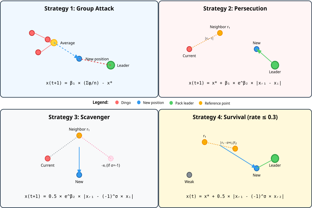
Figure 1. Mathematical modeling of dingo hunting strategies
After a detailed analysis, let's move on to writing the code. The C_AO_DOA_dingo class is an implementation of the DOA optimization algorithm and is derived from the more general C_AO class, implying the presence of inherited functionality to support optimization algorithms. The key characteristics of the class are as follows:
Algorithm parameters:- popSize — population size (number of "dingoes").
- P — probability of choosing between two dingo behavior strategies: hunting or scavenging.
- Q — probability of a group attack or chase.
Initialization: the Init() method is the entry point for initializing the algorithm, accepting ranges of acceptable parameter values, steps for changing them, and the number of epochs (algorithm cycles).
Main loop:
- Moving() — main phase of "movement" or search for a solution by the algorithm, where agents (dingoes) interact and move in the search space.
- Revision () — method is responsible for "revising" decisions made, evaluating results, and adjusting the behavior of agents.
- survival — array storing the "survival" indicators of each agent.
- attackVector — array used to record the indices of agents participating in the attack.
- UpdateSurvivalRates () — update the survival rates of agents.
- GroupAttack () — implement a group attack strategy.
- Persecution () — chasing a prey.
- Scavenger () — scavenging behavior.
- SurvivalProcedure () — execute a procedure related to the agent survival.
Overall, the C_AO_DOA_dingo class models the behavior of a group of dingoes, using their natural instincts of hunting, scavenging, and group interaction to solve optimization problems. It has a flexible parameter system that allows us to customize its behavior, and uses a number of internal methods to simulate the processes that lead to the search for an optimal solution.
//————————————————————————————————————————————————————————————————————
class C_AO_DOA_dingo : public C_AO
{
  public: //----------------------------------------------------------
  ~C_AO_DOA_dingo () { }
  C_AO_DOA_dingo ()
  {
    ao_name = "DOA";
    ao_desc = "Dingo Optimization Algorithm";
    ao_link = "https://www.mql5.com/en/articles/19458";

    popSize = 50;     // population size (number of dingoes)
    P       = 0.5;    // hunting or scavenging probability
    Q       = 0.7;    // group attack or chase probability

    ArrayResize (params, 3);

    params [0].name = "popSize"; params [0].val = popSize;
    params [1].name = "P";       params [1].val = P;
    params [2].name = "Q";       params [2].val = Q;
  }

  void SetParams ()
  {
    popSize = (int)params [0].val;
    P       = params [1].val;
    Q       = params [2].val;
  }

  bool Init (const double &rangeMinP  [],
             const double &rangeMaxP  [],
             const double &rangeStepP [],
             const int     epochsP = 0);

  void Moving   ();
  void Revision ();

  //------------------------------------------------------------------
  double P;          // hunting or scavenging probability
  double Q;          // group attack or chase probability

  private: //---------------------------------------------------------
  double survival []; // array of survival indicators
  int    attackVector []; // array for storing attacker indices

  // Auxiliary methods
  void UpdateSurvivalRates ();
  void GroupAttack         (int agentIdx, int na, double beta1);
  void Persecution         (int agentIdx, double beta1, double beta2);
  void Scavenger           (int agentIdx, double beta2);
  void SurvivalProcedure   (int agentIdx);
};
//————————————————————————————————————————————————————————————————————
The Init method is the entry point for initializing the DOA algorithm. It performs the following key tasks:
Standard initialization:
- The first line calls another method, StandardInit, which performs actions common to all optimization algorithms to configure the parameter search ranges (rangeMinP, rangeMaxP) and the steps for changing them (rangeStepP).
- If the standard initialization fails (returns "false"), the method also terminates.
//————————————————————————————————————————————————————————————————————
//--- Initialization
bool C_AO_DOA_dingo::Init (const double &rangeMinP  [],
                           const double &rangeMaxP  [],
                           const double &rangeStepP [],
                           const int     epochsP = 0)
{
  if (!StandardInit (rangeMinP, rangeMaxP, rangeStepP)) return false;

  ArrayResize     (survival, popSize);
  ArrayInitialize (survival, 1.0);

  // Reserve the maximum size for the attackers' vector
  ArrayResize (attackVector, popSize / 2);

  return true;
}
//————————————————————————————————————————————————————————————————————
The Moving method is the main function that performs one iterative step of the algorithm. It models the behavior of a population of "dingoes" aimed at finding an optimal solution.
First initialization: on the first call, when the "revision" flag is set to 'false', the method randomly distributes values for all parameters (coordinates) of each individual in the population. The ranges and steps for these parameters are specified in advance. After initialization, the "revision" flag is set to 'true' and the method terminates at this step.
Survival assessment: If initialization has already been performed, the method first calls a subroutine to update the "survival" rates of all individuals in the population. This indicator reflects how well the current solution (the individual's position) corresponds to the set goal or how "fit" it is. The method then iterates over each individual in the population.
Two random parameters are generated for the current individual. These parameters influence the specifics of the chosen behavior strategy. Based on probability relationships, an individual chooses one of the strategies:- P probability: if the random number is less than P, the individual switches to the "hunting" strategy.
- Q probability (within the hunt): If an individual chooses "hunting", then with the probability of Q it will use "group attack". During a group attack, an individual moves taking into account the positions of several other individuals in the population. The number of other individuals participating is determined randomly within a certain range.
- Chase (within the hunt): If an individual chooses "hunting" but not "group attack" (with the probability of 1-Q), it will use "chase". When chasing, the individual moves, focusing on the best solutions, attacking the "prey".
- Scavenging (an alternative to hunting): If the random number is greater than or equal to P, the individual chooses the "scavenging" strategy. This strategy simulates the search for remaining prey or random exploration of the solution space.
- Survival testing and adjustment: After applying the main selected strategy (hunting/chase/scavenging), the method checks the survival rate of the current individual. If the survival rate is below a certain threshold (in this case 0.3), a special "survival procedure" is applied. This procedure is aimed at helping a weak individual improve its performance or survive by changing its position.
In this way, the Moving method controls the evolution of the population, allowing each individual to make decisions about its behavior, interact with others, and adapt to conditions, imitating the natural behavior of dingoes.
//————————————————————————————————————————————————————————————————————
//--- Main step of the algorithm
void C_AO_DOA_dingo::Moving ()
{
  // Starting initialization of the population
  if (!revision)
  {
    for (int i = 0; i < popSize; i++)
    {
      for (int j = 0; j < coords; j++)
      {
        a [i].c [j] = u.RNDfromCI (rangeMin [j], rangeMax [j]);
        a [i].c [j] = u.SeInDiSp (a [i].c [j], rangeMin [j], rangeMax [j], rangeStep [j]);
      }
    }
    revision = true;
    return;
  }

  //------------------------------------------------------------------
  // Update survival rates for the entire population
  UpdateSurvivalRates ();

  // Main loop for all dingoes
  for (int i = 0; i < popSize; i++)
  {
    // Generate beta for each agent
    double beta1 = u.RNDfromCI (-2.0, 2.0);
    double beta2 = u.RNDfromCI (-1.0, 1.0);

    // First, choose a strategy
    if (u.RNDprobab () < P)  // Hunt
    {
      if (u.RNDprobab () < Q)  // Group attack
      {
        // Strategy 1: Group attack (Eq. 2)
        int na = 2 + (int)((popSize / 2 - 2) * u.RNDprobab ());
        GroupAttack (i, na, beta1);
      }
      else  // Chase
      {
        // Strategy 2: Chase (Eq. 3)
        Persecution (i, beta1, beta2);
      }
    }
    else  // Scavenging
    {
      // Strategy 3: Scavenging (Eq. 4)
      Scavenger (i, beta2);
    }

    // After the main strategy, check survivability
    if (survival [i] <= 0.3)
    {
      // Strategy 4: Survival procedure for weak individuals (Eq. 6)
      SurvivalProcedure (i);
    }
  }
}
//————————————————————————————————————————————————————————————————————
The following method "GroupAttack" implements one of the main behavior strategies in the algorithm – Strategy 1: Group attack. It simulates a situation where a group of dingoes band together to attack.
Selecting attack participants. The method first determines how many other individuals (dynamic number "na") will participate in the attack together with the current agentIdx individual. It then randomly selects "na" unique index individuals from the entire population. These selected individuals will form the "attack group". It is important that the individuals selected are different to avoid reusing the same individual.
Applying the attack formula. . The method goes through each coordinate (parameter) of the 'c' solution. For each coordinate, it calculates the average value of that coordinate among all individuals included in the attacking group. Then, using this average value, the beta1 parameter (which was generated previously), and the cB[c] value (which represents the current best known solution), a new value is calculated for the current agentIdx individual's coordinate. The position update formula is based on subtracting the product of beta1 and the average coordinate value of the individuals from the best solution.
After calculating a new value for a coordinate, it is brought into line with the permissible boundaries and sampling step, similar to how this was done during initialization.
//————————————————————————————————————————————————————————————————————
//--- Strategy 1: Group attack (Equation 2)
void C_AO_DOA_dingo::GroupAttack (int agentIdx, int na, double beta1)
{
  // x_i(t+1) = beta1 * [sum(phi_k(t))/na] - x*(t)

  // Form a subset of attacking dingoes
  ArrayResize (attackVector, na);
  int count = 0;

  while (count < na)
  {
    int idx = u.RNDintInRange (0, popSize - 1);

    bool unique = true;
    for (int j = 0; j < count; j++)
    {
      if (attackVector [j] == idx)
      {
        unique = false;
        break;
      }
    }

    if (unique)
    {
      attackVector [count++] = idx;
    }
  }

  // Apply the formula
  for (int c = 0; c < coords; c++)
  {
    double sum = 0.0;

    for (int j = 0; j < na; j++)
    {
      sum += a [attackVector [j]].c [c];
    }

    //a [agentIdx].c [c] = beta1 * (sum / na) - cB [c];
    a [agentIdx].c [c] = cB [c] - beta1 * (sum / na);
    a [agentIdx].c [c] = u.SeInDiSp (a [agentIdx].c [c], rangeMin [c], rangeMax [c], rangeStep [c]);
  }
}
//————————————————————————————————————————————————————————————————————
The Persecution method implements Strategy 2 based on chasing ("persecuting") some target object. The strategy is designed to update the position of one specific individual in the population. The method first selects a random other individual from the population. This individual will be called the "attacker" (r1). It is important that the attacking individual is not the same individual we are updating (that is, agentIdx should not match r1).
The "chase" strategy attempts to move the target individual (agentIdx) in the direction determined by the combination of the best solution found (cB) and the difference between a random other individual and the target individual itself.
- cB (best solution) ensures that the movement is directed towards the best known solution.
- beta1 and exp (beta2), these parameters control the "strength" or "range" of the chase step. A larger "beta1" or "beta2" will result in larger shifts.
- |x_r1 (t) - x_i (t)| (difference) determines how far away another individual is. The greater the difference, the stronger the chase effect.
Thus, this strategy models the behavior when one individual (or, more correctly, its actions) tries to "catch up" or get closer to another equally random individual, but all this dynamics are shifted towards the best solution found in the population.
//————————————————————————————————————————————————————————————————————
//--- Strategy 2: Chase (Equation 3)
void C_AO_DOA_dingo::Persecution (int agentIdx, double beta1, double beta2)
{
  // x_i(t+1) = x*(t) + beta1 * exp(beta2) * |x_r1(t) - x_i(t)|

  int r1;
  do
  {
    r1 = u.RNDintInRange (0, popSize - 1);
  }
  while (r1 == agentIdx);

  double expBeta2 = MathExp (beta2);

  for (int c = 0; c < coords; c++)
  {
    double diff = MathAbs (a [r1].c [c] - a [agentIdx].c [c]);
    a [agentIdx].c [c] = cB [c] + beta1 * expBeta2 * diff;
    a [agentIdx].c [c] = u.SeInDiSp (a [agentIdx].c [c], rangeMin [c], rangeMax [c], rangeStep [c]);
  }
}
//————————————————————————————————————————————————————————————————————
The Scavenger method describes Strategy 3: Scavenging, imitating the behavior of a scavenging individual (dingo). First, the method randomly selects another individual (r1) from the entire population. This individual becomes an "object of interest" for the search. The selected individual cannot be the same as the current individual performing the search. A random "sigma" character is used to determine the search direction. This sign can be either +1 or -1, chosen randomly. This adds an element of unpredictability to the search direction.
Next, for each characteristic (coordinate) of the solution: the difference between the value of this characteristic in another individual and in the current individual is calculated, multiplied by a randomly selected "sigma" sign. This means that the current position of an individual is either added to or subtracted from the position of another individual. From this difference, the absolute value (MathAbs) is taken to obtain the distance value.
This absolute difference is multiplied by half the exponent of "beta2", this parameter, raised to a power, determines how much the position will change. A multiplier of 0.5 scales this influence. The resulting value from the multiplication becomes the new coordinate for the current individual. As with other methods, the new coordinate value is then constrained to the acceptable limits defined by "rangeMin", "rangeMax" and "rangeStep".
The "Scavenging" strategy encourages an individual to move a distance depending on the difference between its own position and the position of another individual, and this direction can be either "ahead" or "behind" the current individual, determined by the random "sigma" sign. The strength of this movement is also adjusted via the beta2 parameter. This strategy adds an element of more random and perhaps less targeted searching, simulating behavior where an individual might follow prey trails or search for carcasses.
//————————————————————————————————————————————————————————————————————
//--- Strategy 3: Scavenging (Equation 4)
void C_AO_DOA_dingo::Scavenger (int agentIdx, double beta2)
{
  // x_i(t+1) = 0.5 * exp(beta2) * |x_r1(t) - (-1)^sigma * x_i(t)|

  int r1;
  do
  {
    r1 = u.RNDintInRange (0, popSize - 1);
  }
  while (r1 == agentIdx);

  double sigma = u.RNDbool () ? 1.0 : -1.0;
  double halfExpBeta2 = 0.5 * MathExp (beta2);

  for (int c = 0; c < coords; c++)
  {
    double diff = MathAbs (a [r1].c [c] - sigma * a [agentIdx].c [c]);
    a [agentIdx].c [c] = halfExpBeta2 * diff;
    a [agentIdx].c [c] = u.SeInDiSp (a [agentIdx].c [c], rangeMin [c], rangeMax [c], rangeStep [c]);
  }
}
//————————————————————————————————————————————————————————————————————
The SurvivalProcedure describes Strategy 4: Survival procedure. It simulates a scenario in which an individual (dingo) updates its position in an attempt to survive or improve its chances based on the position of other individuals.
The method selects two different individuals (r1 and r2) from the population, each of which is necessarily different from the current individual performing the survival procedure (agentIdx). Also, these two selected individuals should be different from each other.
For each characteristic (coordinate) a random change of sign (sigma) is performed. This sign can be either +1 or -1, chosen randomly. This determines whether the second individual (r2) is included in the calculation directly or with an inverted value. For each coordinate:
- the difference between the corresponding characteristics of the selected first individual (a [r1].c [c]) and the second individual (a [r2].c [c]) is calculated, to which the random sign "sigma" is applied;
- the absolute value of this difference (diff) is taken;
- the obtained absolute difference is multiplied by 0.5;
- half of this difference is added to the current best known solution (cB [c]). This means that the individual's new position shifts away from the best solution in the direction determined by the difference between the other two individuals. The calculated new value becomes the new coordinate for the current individual;
- as in the previous methods, the obtained coordinate value is then adjusted to stay within acceptable limits.
The "Survival" strategy is a mechanism where an individual updates its position using information from two other individuals. The position update occurs as a shift from the current best solution (cB), where the magnitude and direction of this shift depend on the difference in positions of the two random individuals. This can be interpreted as searching for a "niche" or "resource" that is somewhere in between two other individuals, but with some randomness in determining exactly where to move.
//————————————————————————————————————————————————————————————————————
//--- Strategy 4: Survival procedure (Equation 6)
void C_AO_DOA_dingo::SurvivalProcedure (int agentIdx)
{
  // x_i(t) = x*(t) + 0.5 * |x_r1(t) - (-1)^sigma * x_r2(t)|

  int r1, r2;

  r1 = u.RNDintInRange (0, popSize - 1);
  while (r1 == agentIdx)
  {
    r1 = u.RNDintInRange (0, popSize - 1);
  }

  r2 = u.RNDintInRange (0, popSize - 1);
  while (r2 == agentIdx || r2 == r1)
  {
    r2 = u.RNDintInRange (0, popSize - 1);
  }

  double sigma = u.RNDbool () ? 1.0 : -1.0;

  for (int c = 0; c < coords; c++)
  {
    double diff = MathAbs (a [r1].c [c] - sigma * a [r2].c [c]);
    a [agentIdx].c [c] = cB [c] + 0.5 * diff;
    a [agentIdx].c [c] = u.SeInDiSp (a [agentIdx].c [c], rangeMin [c], rangeMax [c], rangeStep [c]);
  }
}
//————————————————————————————————————————————————————————————————————
The UpdateSurvivalRates method is responsible for updating survival metrics for each individual in the population. This is an important step that helps determine how likely it is that each individual will be able to "survive" and maintain its position (or, conversely, be discarded) in the process of evolution.
The method first runs through all individuals in the population to determine two extreme values: the minimum fitness (minFitness) and the maximum fitness (maxFitness). In this case, the first individual is taken as an initial guess for these values. The range between the maximum and minimum fitness is then calculated. This range reflects the variability of solution quality in the current population.
If the fitness range is zero (meaning that all individuals have the same fitness), then the survival rate for each individual is set to 0.5. In this case, the assumption is made that all individuals have an equal chance of survival, since there is no clear leader or outsider.
If the fitness range is not equal to zero, then for each individual its survival rate (survival [i]) is calculated using the formula: (maximum fitness - fitness of the current individual) / fitness range.
The method normalizes each individual's fitness to the best and worst in the population, converting it into a score that will then be used by other parts of the algorithm to make decisions about which individuals should change their positions more actively and which should be preserved.
//————————————————————————————————————————————————————————————————————
//--- Update survival stats (Equation 5)
void C_AO_DOA_dingo::UpdateSurvivalRates ()
{
  // survival(i) = (fitness_max - fitness(i)) / (fitness_max - fitness_min)

  double minFitness = a [0].f;
  double maxFitness = a [0].f;

  for (int i = 1; i < popSize; i++)
  {
    if (a [i].f < minFitness) minFitness = a [i].f;
    if (a [i].f > maxFitness) maxFitness = a [i].f;
  }

  double range = maxFitness - minFitness;

  if (range < DBL_EPSILON)
  {
    ArrayInitialize (survival, 0.5);
  }
  else
  {
    for (int i = 0; i < popSize; i++)
    {
      survival [i] = (maxFitness - a [i].f) / range;
    }
  }
}
//————————————————————————————————————————————————————————————————————
The Revision method is critical to most heuristic optimization algorithms. Its task is to save the best solution found at a given (or any previous) point in time. This ensures that the algorithm will not "forget" a good solution, even if other individuals evolve and perhaps find solutions that temporarily appear less successful. Thus, fB and cB always store the best fitness configuration found and its corresponding coordinates.
//————————————————————————————————————————————————————————————————————
//--- Update the best solution
void C_AO_DOA_dingo::Revision ()
{
  for (int i = 0; i < popSize; i++)
  {
    if (a [i].f > fB)
    {
      fB = a [i].f;
      ArrayCopy (cB, a [i].c, 0, 0, WHOLE_ARRAY);
    }
  }
}
//————————————————————————————————————————————————————————————————————
After implementing such a promising and multifaceted optimization method, we can finally begin testing.
Test results
According to the test results, the algorithm scored 35% of the possible 100%. Unfortunately, expectations were not entirely met.
=============================
5 Hilly's; Func runs: 10000; result: 0.49066480903390775
25 Hilly's; Func runs: 10000; result: 0.399914179876301
500 Hilly's; Func runs: 10000; result: 0.35798310869836164
=============================
5 Forest's; Func runs: 10000; result: 0.29643143556801427
25 Forest's; Func runs: 10000; result: 0.20458050042664944
500 Forest's; Func runs: 10000; result: 0.17091405461356773
=============================
5 Megacity's; Func runs: 10000; result: 0.36615384615384616
25 Megacity's; Func runs: 10000; result: 0.4489230769230771
500 Megacity's; Func runs: 10000; result: 0.45393846153845924
=============================
All score: 3.18950 (35.44%)
The visualization shows how the algorithm's strategies change based on the complex pattern of agent movements. Overall, the strange distribution of agent individuals along the "diagonal" of the search space indicates a possible error in the internal logic of the algorithm, made by the authors.
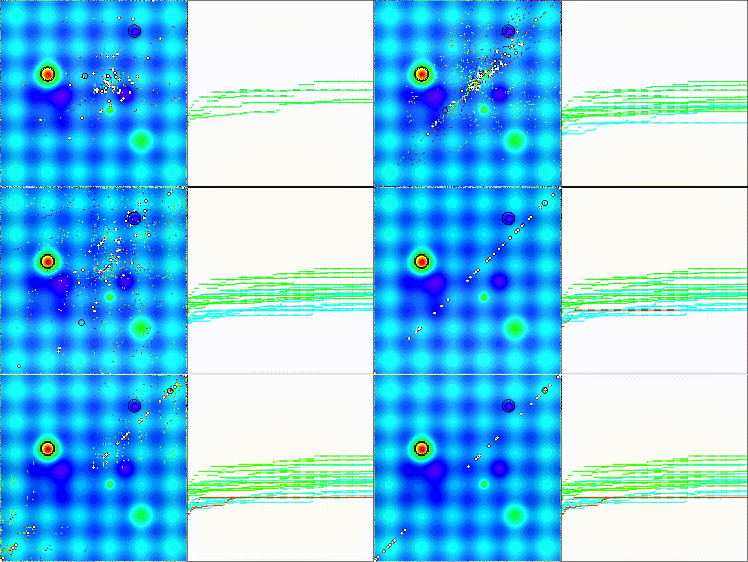
DOA_dingo on the Hilly test function
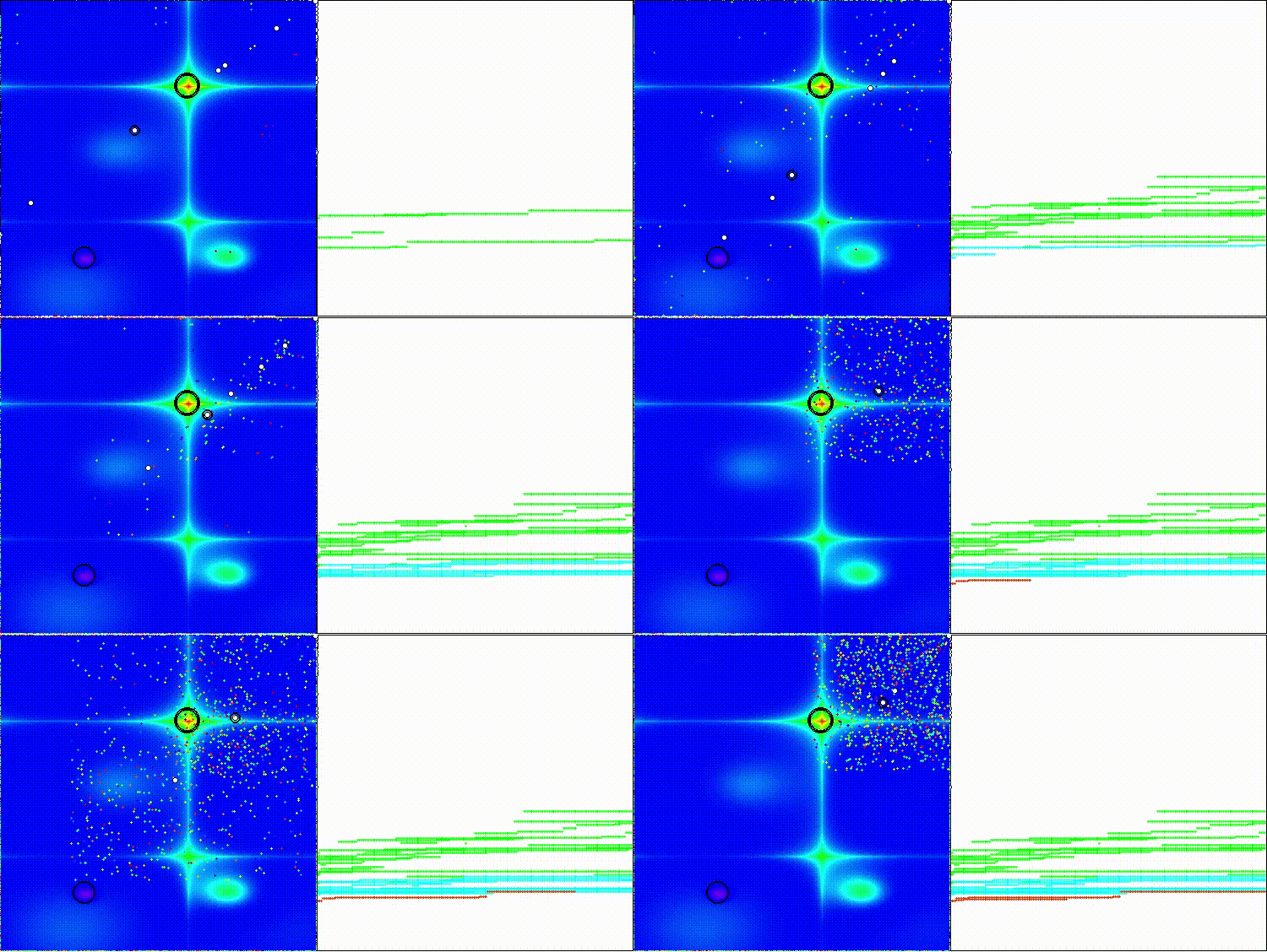
DOA_dingo on the Forest test function
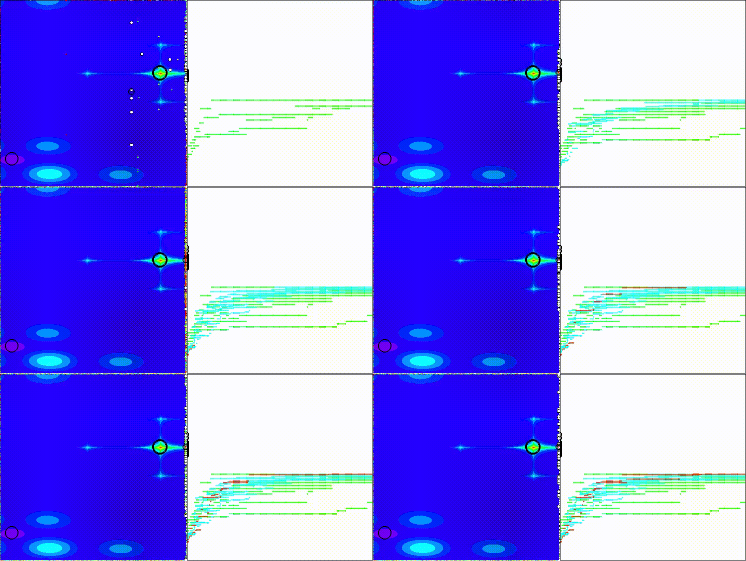
DOA_dingo on the Megacity test function
The DOA_dingo algorithm is presented in the rating table for informational purposes after the test.
| # | AO | Description | Hilly | Hilly Final | Forest | Forest Final | Megacity (discrete) | Megacity Final | Final Result | % of MAX | ||||||
| 10 p (5 F) | 50 p (25 F) | 1000 p (500 F) | 10 p (5 F) | 50 p (25 F) | 1000 p (500 F) | 10 p (5 F) | 50 p (25 F) | 1000 p (500 F) | ||||||||
| 1 | ANS | across neighbourhood search | 0.94948 | 0.84776 | 0.43857 | 2.23581 | 1.00000 | 0.92334 | 0.39988 | 2.32323 | 0.70923 | 0.63477 | 0.23091 | 1.57491 | 6.134 | 68.15 |
| 2 | CLA | code lock algorithm (joo) | 0.95345 | 0.87107 | 0.37590 | 2.20042 | 0.98942 | 0.91709 | 0.31642 | 2.22294 | 0.79692 | 0.69385 | 0.19303 | 1.68380 | 6.107 | 67.86 |
| 3 | AMOm | animal migration ptimization M | 0.90358 | 0.84317 | 0.46284 | 2.20959 | 0.99001 | 0.92436 | 0.46598 | 2.38034 | 0.56769 | 0.59132 | 0.23773 | 1.39675 | 5.987 | 66.52 |
| 4 | (P+O)ES | (P+O) evolution strategies | 0.92256 | 0.88101 | 0.40021 | 2.20379 | 0.97750 | 0.87490 | 0.31945 | 2.17185 | 0.67385 | 0.62985 | 0.18634 | 1.49003 | 5.866 | 65.17 |
| 5 | CTA | comet tail algorithm (joo) | 0.95346 | 0.86319 | 0.27770 | 2.09435 | 0.99794 | 0.85740 | 0.33949 | 2.19484 | 0.88769 | 0.56431 | 0.10512 | 1.55712 | 5.846 | 64.96 |
| 6 | TETA | time evolution travel algorithm (joo) | 0.91362 | 0.82349 | 0.31990 | 2.05701 | 0.97096 | 0.89532 | 0.29324 | 2.15952 | 0.73462 | 0.68569 | 0.16021 | 1.58052 | 5.797 | 64.41 |
| 7 | SDSm | stochastic diffusion search M | 0.93066 | 0.85445 | 0.39476 | 2.17988 | 0.99983 | 0.89244 | 0.19619 | 2.08846 | 0.72333 | 0.61100 | 0.10670 | 1.44103 | 5.709 | 63.44 |
| 8 | BOAm | billiards optimization algorithm M | 0.95757 | 0.82599 | 0.25235 | 2.03590 | 1.00000 | 0.90036 | 0.30502 | 2.20538 | 0.73538 | 0.52523 | 0.09563 | 1.35625 | 5.598 | 62.19 |
| 9 | AAm | archery algorithm M | 0.91744 | 0.70876 | 0.42160 | 2.04780 | 0.92527 | 0.75802 | 0.35328 | 2.03657 | 0.67385 | 0.55200 | 0.23738 | 1.46323 | 5.548 | 61.64 |
| 10 | ESG | evolution of social groups (joo) | 0.99906 | 0.79654 | 0.35056 | 2.14616 | 1.00000 | 0.82863 | 0.13102 | 1.95965 | 0.82333 | 0.55300 | 0.04725 | 1.42358 | 5.529 | 61.44 |
| 11 | SIA | simulated isotropic annealing (joo) | 0.95784 | 0.84264 | 0.41465 | 2.21513 | 0.98239 | 0.79586 | 0.20507 | 1.98332 | 0.68667 | 0.49300 | 0.09053 | 1.27020 | 5.469 | 60.76 |
| 12 | EOm | extremal_optimization_M | 0.76166 | 0.77242 | 0.31747 | 1.85155 | 0.99999 | 0.76751 | 0.23527 | 2.00277 | 0.74769 | 0.53969 | 0.14249 | 1.42987 | 5.284 | 58.71 |
| 13 | BBO | biogeography based optimization | 0.94912 | 0.69456 | 0.35031 | 1.99399 | 0.93820 | 0.67365 | 0.25682 | 1.86867 | 0.74615 | 0.48277 | 0.17369 | 1.40261 | 5.265 | 58.50 |
| 14 | ACS | artificial cooperative search | 0.75547 | 0.74744 | 0.30407 | 1.80698 | 1.00000 | 0.88861 | 0.22413 | 2.11274 | 0.69077 | 0.48185 | 0.13322 | 1.30583 | 5.226 | 58.06 |
| 15 | DA | dialectical algorithm | 0.86183 | 0.70033 | 0.33724 | 1.89940 | 0.98163 | 0.72772 | 0.28718 | 1.99653 | 0.70308 | 0.45292 | 0.16367 | 1.31967 | 5.216 | 57.95 |
| 16 | BHAm | black hole algorithm M | 0.75236 | 0.76675 | 0.34583 | 1.86493 | 0.93593 | 0.80152 | 0.27177 | 2.00923 | 0.65077 | 0.51646 | 0.15472 | 1.32195 | 5.196 | 57.73 |
| 17 | ASO | anarchy society optimization | 0.84872 | 0.74646 | 0.31465 | 1.90983 | 0.96148 | 0.79150 | 0.23803 | 1.99101 | 0.57077 | 0.54062 | 0.16614 | 1.27752 | 5.178 | 57.54 |
| 18 | RFO | royal flush optimization (joo) | 0.83361 | 0.73742 | 0.34629 | 1.91733 | 0.89424 | 0.73824 | 0.24098 | 1.87346 | 0.63154 | 0.50292 | 0.16421 | 1.29867 | 5.089 | 56.55 |
| 19 | AOSm | atomic orbital search M | 0.80232 | 0.70449 | 0.31021 | 1.81702 | 0.85660 | 0.69451 | 0.21996 | 1.77107 | 0.74615 | 0.52862 | 0.14358 | 1.41835 | 5.006 | 55.63 |
| 20 | TSEA | turtle shell evolution algorithm (joo) | 0.96798 | 0.64480 | 0.29672 | 1.90949 | 0.99449 | 0.61981 | 0.22708 | 1.84139 | 0.69077 | 0.42646 | 0.13598 | 1.25322 | 5.004 | 55.60 |
| 21 | BSA | backtracking_search_algorithm | 0.97309 | 0.54534 | 0.29098 | 1.80941 | 0.99999 | 0.58543 | 0.21747 | 1.80289 | 0.84769 | 0.36953 | 0.12978 | 1.34700 | 4.959 | 55.10 |
| 22 | DE | differential evolution | 0.95044 | 0.61674 | 0.30308 | 1.87026 | 0.95317 | 0.78896 | 0.16652 | 1.90865 | 0.78667 | 0.36033 | 0.02953 | 1.17653 | 4.955 | 55.06 |
| 23 | SRA | successful restaurateur algorithm (joo) | 0.96883 | 0.63455 | 0.29217 | 1.89555 | 0.94637 | 0.55506 | 0.19124 | 1.69267 | 0.74923 | 0.44031 | 0.12526 | 1.31480 | 4.903 | 54.48 |
| 24 | CRO | chemical reaction optimization | 0.94629 | 0.66112 | 0.29853 | 1.90593 | 0.87906 | 0.58422 | 0.21146 | 1.67473 | 0.75846 | 0.42646 | 0.12686 | 1.31178 | 4.892 | 54.36 |
| 25 | BIO | blood inheritance optimization (joo) | 0.81568 | 0.65336 | 0.30877 | 1.77781 | 0.89937 | 0.65319 | 0.21760 | 1.77016 | 0.67846 | 0.47631 | 0.13902 | 1.29378 | 4.842 | 53.80 |
| 26 | DOA | dream_optimization_algorithm | 0.85556 | 0.70085 | 0.37280 | 1.92921 | 0.73421 | 0.48905 | 0.24147 | 1.46473 | 0.77231 | 0.47354 | 0.18561 | 1.43146 | 4.825 | 53.62 |
| 27 | BSA | bird swarm algorithm | 0.89306 | 0.64900 | 0.26250 | 1.80455 | 0.92420 | 0.71121 | 0.24939 | 1.88479 | 0.69385 | 0.32615 | 0.10012 | 1.12012 | 4.809 | 53.44 |
| 28 | DEA | dolphin_echolocation_algorithm | 0.75995 | 0.67572 | 0.34171 | 1.77738 | 0.89582 | 0.64223 | 0.23941 | 1.77746 | 0.61538 | 0.44031 | 0.15115 | 1.20684 | 4.762 | 52.91 |
| 29 | HS | harmony search | 0.86509 | 0.68782 | 0.32527 | 1.87818 | 0.99999 | 0.68002 | 0.09590 | 1.77592 | 0.62000 | 0.42267 | 0.05458 | 1.09725 | 4.751 | 52.79 |
| 30 | SSG | saplings sowing and growing | 0.77839 | 0.64925 | 0.39543 | 1.82308 | 0.85973 | 0.62467 | 0.17429 | 1.65869 | 0.64667 | 0.44133 | 0.10598 | 1.19398 | 4.676 | 51.95 |
| 31 | BCOm | bacterial chemotaxis optimization M | 0.75953 | 0.62268 | 0.31483 | 1.69704 | 0.89378 | 0.61339 | 0.22542 | 1.73259 | 0.65385 | 0.42092 | 0.14435 | 1.21912 | 4.649 | 51.65 |
| 32 | ABO | african buffalo optimization | 0.83337 | 0.62247 | 0.29964 | 1.75548 | 0.92170 | 0.58618 | 0.19723 | 1.70511 | 0.61000 | 0.43154 | 0.13225 | 1.17378 | 4.634 | 51.49 |
| 33 | (PO)ES | (PO) evolution strategies | 0.79025 | 0.62647 | 0.42935 | 1.84606 | 0.87616 | 0.60943 | 0.19591 | 1.68151 | 0.59000 | 0.37933 | 0.11322 | 1.08255 | 4.610 | 51.22 |
| 34 | FBA | fractal-based Algorithm | 0.79000 | 0.65134 | 0.28965 | 1.73099 | 0.87158 | 0.56823 | 0.18877 | 1.62858 | 0.61077 | 0.46062 | 0.12398 | 1.19537 | 4.555 | 50.61 |
| 35 | TSm | tabu search M | 0.87795 | 0.61431 | 0.29104 | 1.78330 | 0.92885 | 0.51844 | 0.19054 | 1.63783 | 0.61077 | 0.38215 | 0.12157 | 1.11449 | 4.536 | 50.40 |
| 36 | BSO | brain storm optimization | 0.93736 | 0.57616 | 0.29688 | 1.81041 | 0.93131 | 0.55866 | 0.23537 | 1.72534 | 0.55231 | 0.29077 | 0.11914 | 0.96222 | 4.498 | 49.98 |
| 37 | WOAm | wale optimization algorithm M | 0.84521 | 0.56298 | 0.26263 | 1.67081 | 0.93100 | 0.52278 | 0.16365 | 1.61743 | 0.66308 | 0.41138 | 0.11357 | 1.18803 | 4.476 | 49.74 |
| 38 | AEFA | artificial electric field algorithm | 0.87700 | 0.61753 | 0.25235 | 1.74688 | 0.92729 | 0.72698 | 0.18064 | 1.83490 | 0.66615 | 0.11631 | 0.09508 | 0.87754 | 4.459 | 49.55 |
| 39 | AEO | artificial ecosystem-based optimization algorithm | 0.91380 | 0.46713 | 0.26470 | 1.64563 | 0.90223 | 0.43705 | 0.21400 | 1.55327 | 0.66154 | 0.30800 | 0.28563 | 1.25517 | 4.454 | 49.49 |
| 40 | CAm | camel algorithm M | 0.78684 | 0.56042 | 0.35133 | 1.69859 | 0.82772 | 0.56041 | 0.24336 | 1.63149 | 0.64846 | 0.33092 | 0.13418 | 1.11356 | 4.444 | 49.37 |
| 41 | ACOm | ant colony optimization M | 0.88190 | 0.66127 | 0.30377 | 1.84693 | 0.85873 | 0.58680 | 0.15051 | 1.59604 | 0.59667 | 0.37333 | 0.02472 | 0.99472 | 4.438 | 49.31 |
| 42 | CMAES | covariance_matrix_adaptation_evolution_strategy | 0.76258 | 0.72089 | 0.00000 | 1.48347 | 0.82056 | 0.79616 | 0.00000 | 1.61672 | 0.75846 | 0.49077 | 0.00000 | 1.24923 | 4.349 | 48.33 |
| 43 | DA_duelist | duelist_algorithm | 0.92782 | 0.53778 | 0.27792 | 1.74352 | 0.86957 | 0.47536 | 0.18193 | 1.52686 | 0.62153 | 0.33569 | 0.11715 | 1.07437 | 4.345 | 48.28 |
| 44 | BFO-GA | bacterial foraging optimization - ga | 0.89150 | 0.55111 | 0.31529 | 1.75790 | 0.96982 | 0.39612 | 0.06305 | 1.42899 | 0.72667 | 0.27500 | 0.03525 | 1.03692 | 4.224 | 46.93 |
| 45 | SOA | simple optimization algorithm | 0.91520 | 0.46976 | 0.27089 | 1.65585 | 0.89675 | 0.37401 | 0.16984 | 1.44060 | 0.69538 | 0.28031 | 0.10852 | 1.08422 | 4.181 | 46.45 |
| DOA_dingo | dingo_optimization_algorithm | 0.49066 | 0.39991 | 0.35798 | 1.24855 | 0.29643 | 0.20458 | 0.17091 | 0.67192 | 0.36615 | 0.44892 | 0.45394 | 1.26901 | 3.189 | 35.44 | |
| RW | random walk | 0.48754 | 0.32159 | 0.25781 | 1.06694 | 0.37554 | 0.21944 | 0.15877 | 0.75375 | 0.27969 | 0.14917 | 0.09847 | 0.52734 | 2.348 | 26.09 | |
Summary
In this article, we have considered an interesting optimization algorithm, noteworthy in terms of the approaches used. At first glance, the algorithm may not seem like the best way to find the optimal solution. However, during numerous experiments, an unexpected potential emerged: with proper refinement of the ideas embedded in DOA, the algorithm is capable of demonstrating very respectable results — at the level of the best population-based methods.
We will discuss exactly what was discovered in the next article. Additionally, a small gift awaits the most attentive optimization enthusiasts: a small modification to the algorithm code may be found in the file, which has already significantly impacted the results. Please share your thoughts in the comments.
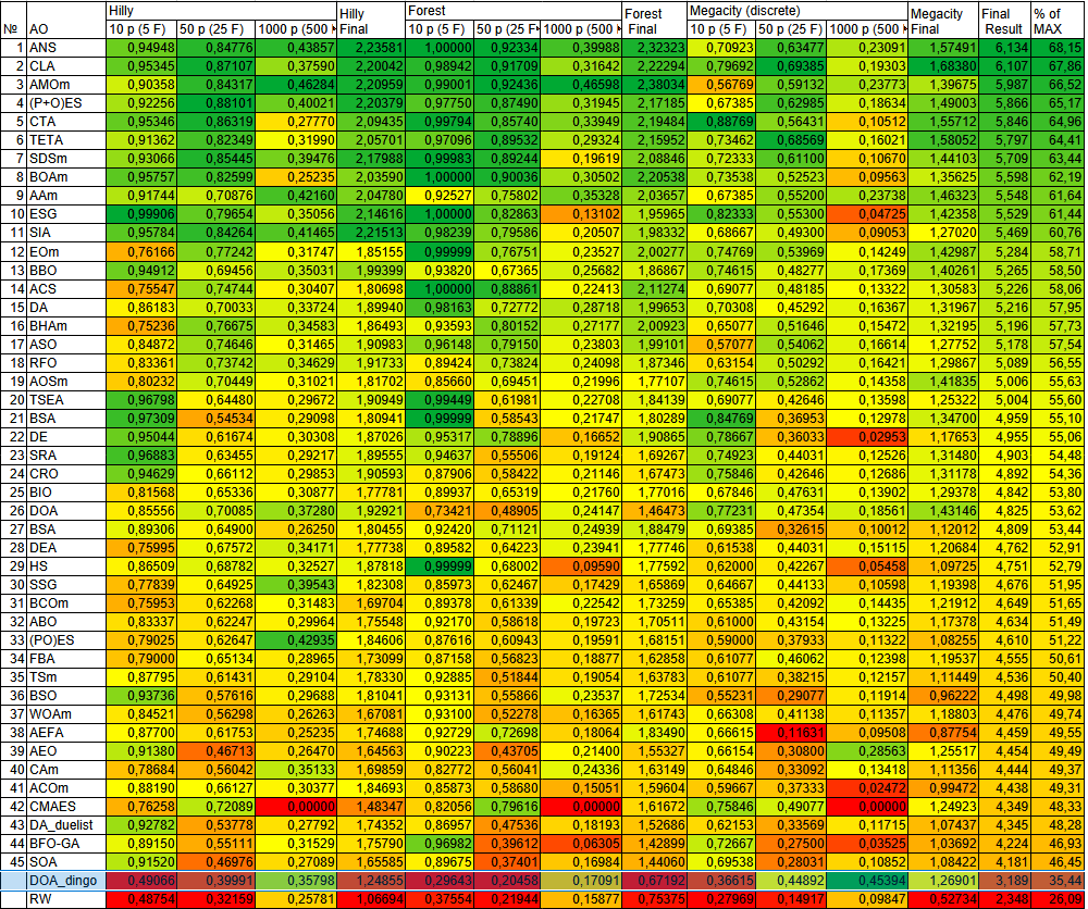
Figure 2. Color-coded comparison of algorithms across the corresponding tests
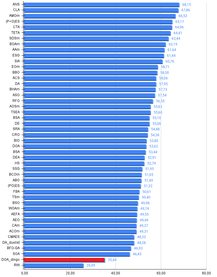
Figure 3. Histogram of algorithm testing results (scale from 0 to 100, the higher the better, where 100 is the maximum possible theoretical result, in the archive there is a script for calculating the rating table)
DOA_dingo pros and cons:
Pros:
- Fast.
Disadvantages:
- High variance in results.
- Weak exploration of the search space.
The article is accompanied by an archive with the current versions of the algorithm codes. The author of the article is not responsible for the absolute accuracy in the description of canonical algorithms. Changes have been made to many of them to improve search capabilities. The conclusions and judgments presented in the articles are based on the results of the experiments.
Programs used in the article
| # | Name | Type | Description |
|---|---|---|---|
| 1 | #C_AO.mqh | Include | Parent class of population optimization algorithms |
| 2 | #C_AO_enum.mqh | Include | Enumeration of population optimization algorithms |
| 3 | TestFunctions.mqh | Include | Library of test functions |
| 4 | TestStandFunctions.mqh | Include | Test stand function library |
| 5 | Utilities.mqh | Include | Library of auxiliary functions |
| 6 | CalculationTestResults.mqh | Include | Script for calculating results in the comparison table |
| 7 | Testing AOs.mq5 | Script | The unified test stand for all population optimization algorithms |
| 8 | Simple use of population optimization algorithms.mq5 | Script | A simple example of using population optimization algorithms without visualization |
| 9 | Test_AO_DOA_dingo.mq5 | Script | DOA_dingo test stand |
Translated from Russian by MetaQuotes Ltd.
Original article: https://www.mql5.com/ru/articles/19458
Warning: All rights to these materials are reserved by MetaQuotes Ltd. Copying or reprinting of these materials in whole or in part is prohibited.
This article was written by a user of the site and reflects their personal views. MetaQuotes Ltd is not responsible for the accuracy of the information presented, nor for any consequences resulting from the use of the solutions, strategies or recommendations described.

 Constructing a Trade Replay Engine in MQL5: Stepping Through Historical Trades Bar by Bar for Manual Review
 Online Linear Regression with Recursive Least Squares in MQL5: A Parameter-Free Adaptive Trend Estimator
 Mapping Dealer Gamma Exposure (GEX) in MetaTrader 5: Walls, the Zero-Gamma Flip, and a Chart Overlay
 How To Profile MQL5 Code in MetaEditor

- Free trading apps
- Over 8,000 signals for copying
- Economic news for exploring financial markets
You agree to website policy and terms of use