

Bonobo Optimizer (BO)
 1 268
1 268
 0
0

Contents
Introduction
Let us examine another interesting and promising optimization method known as the Bonobo Optimizer. The BO algorithm was published in 2021; its authors are Amit Kumar Das and Dilip Kumar Pratihar. The method is based on the social behavior of bonobos, which lead complex social lives with several unique characteristics. Imagine a population in which each bonobo represents one possible solution to an optimization problem.
Implementation of the Algorithm
The main idea behind the BO algorithm is the dynamic "fission-fusion" social structure, which means that individuals do not always act as a single group; instead, they form temporary subgroups for different activities. The best bonobo in the population is called the alpha bonobo; it is the current best solution found, which all the others strive to reach.
The BO algorithm implements three different mating strategies that mimic the actual behavior of bonobos. The first strategy is a randomized choice, in which a bonobo produces an offspring by moving simultaneously toward the alpha bonobo (the best solution) and toward a random partner from the subgroup. For example, if the current bonobo is at point X=5, the alpha is at X=10, and a random partner is at X=7, then the offspring may end up roughly at X=7.5, taking a step toward the best solution while incorporating a bit of diversity from the partner. The coefficients scab=1.25 and scsb=1.3 control the size of these steps; they can be greater than one, which sometimes allows the algorithm to jump over the best solution in order to explore the region beyond it.
The second strategy is “extra-group mating,” which occurs with low probability and mimics a situation in which a bonobo seeks a mate from another group. In this case, an offspring is created using information about the population boundaries — the locations of the most extreme bonobos for each coordinate. The algorithm examines the position of the alpha bonobo relative to the current individual and decides whether to move toward the upper or lower bound of the range, using exponential "beta" coefficients that create nonlinear jumps in the solution space. For example, if the alpha bonobo is to the right of the current bonobo, the offspring jumps to the right toward the upper bound; if the alpha bonobo is to the left, it jumps to the left toward the lower bound. This helps explore the outer regions of the search space.
The third strategy is "consortship mating," in which two bonobos form a temporary pair and an offspring is created as a combination of their positions through directed movement. The "direction" flag plays an important role here; it is determined by comparing the fitness of the current bonobo and its partner. If the current bonobo is better than its partner, then direction=1 and the movement is away from the partner; if it is worse, then direction=-1 and the movement is toward the partner. For example, if two bonobos are at points X=5 and X=8, and the first is better, then the offspring is created approximately at X=4 or X=6, moving away from the worse partner; and if the first is worse, then the offspring will be closer to X=8, moving toward the better of the two solutions. The "exp(-random)" coefficient creates decaying steps that decrease over time.
A critically important mechanism in the algorithm is the "acceptance criterion" for a new solution. Bonobos do not always accept an offspring they have created — a new solution is accepted only if it is better than the current one, or, with a small probability, it is accepted by chance even if it is worse. This prevents the population from deteriorating and ensures that poor solutions do not crowd out good ones. For example, if a bonobo has a fitness of 0.8 and its offspring has a fitness of 0.7, then in 97 percent of cases the offspring is rejected and the bonobo remains in its current position; only in 3 percent of cases is the offspring accepted to maintain population diversity. If the offspring is better (fitness 0.9), it is always accepted.
The algorithm uses an adaptive system of positive and negative phases that automatically adjusts the parameters based on the progress of the optimization. When a new, better solution is found, the "positive phase" begins: the "ppc" counter increases, the randomized mating probability rises, making this strategy more aggressive (it can reach 1.0), the subgroup size increases for a broader search, and the probability of extra-group mating returns to its minimum of 3 percent. This is a period of intensive exploitation of the promising area that has been identified.
When several iterations pass without improvement, a "negative phase" begins: the "npc" counter increases, the probability of randomized partner selection decreases (it may drop to 0), the subgroup size decreases for a more cautious search, and the probability of extra-group mating increases to 50 percent. This is a period of intensified "exploration," during which the algorithm attempts to find new promising areas within the search space. The rate of these changes is controlled by the "rcpp" parameter, which is typically around 0.0035; this means that the parameters change gradually rather than in sudden jumps.
For example, imagine finding the maximum of a function on a plane, where the optimum lies at the top of a hill. At the beginning, 30 bonobos are scattered randomly across the entire plane. At each iteration, every bonobo forms a subgroup of 3–5 neighbors, selects the best partner from the subgroup, creates an offspring using one of three mating strategies, and, if the offspring is better, moves to its position.
The alpha bonobo is continually updated whenever any bonobo finds a better point. Suppose one bonobo happens to be near the top of the hill, and its fitness improves — it becomes the alpha, a positive phase begins, and all the other bonobos start actively moving toward it, producing offspring in the direction of the alpha; subgroups grow larger, encompassing a larger portion of the population, the probability of randomized mating rises to 70–80 percent, and the population rapidly converges toward the area around the summit.
If no improvements are observed after 50 iterations, a negative phase begins: randomized mating drops to 30–40 percent, while extra-group mating increases to 20–30 percent, and bonobos begin making longer jumps, exploring other parts of the landscape in case there is another, higher peak. The “acceptance criteria” ensure that even during periods of active jumping, bonobos do not abandon good positions they have found without good reason — they try new points, but return if the new point is worse.
An important detail is the use of normalized weights that sum to one; this creates a convex combination of positions and ensures that the offspring does not stray too far from its parents. In addition, boundary handling via “clipping” strictly clips the coordinates if they exceed the allowable limits. The exponential “beta” coefficients are calculated using the formula: exp(r^2 + r - 2/r), where “r” is a random number. The formula is specifically designed to generate coefficients in the range from 0.1 to 3 with a heavy-tailed distribution, which allows occasional very large jumps to escape local optima. This is very reminiscent of price behavior when a sharp spike occurs and the movement pushes us to a new level. The “direction” parameter, multiplied by “exp(-random),” creates directed movement with exponentially decreasing strength, which mimics the time-dependent decay of activity observed in real bonobos.
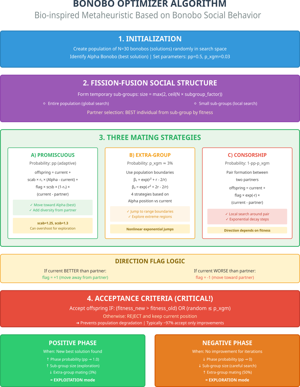
Figure 1. Flowchart of the BO algorithm
The diagram includes: Initialization — initial population and parameters; Fission-Fusion — dynamic subgroups; Three Mating Strategies — all three types of mating with formulas; Direction Flag Logic — direction flag logic; Acceptance Criteria — critical selection mechanism (in red); and Positive/Negative Phases — adaptive modes. Let's move on to writing the pseudocode for the BO algorithm.
INITIALIZATION
Create a population of thirty bonobos with random positions within the allowed
bounds and calculate their fitness. The best individual becomes the alpha bonobo.
Set the initial parameters: the randomized mating probability is
one half, the extra-group mating probability is three percent, the phase counters are set to zero, and the subgroup
size factor is set to a medium level.
MAIN LOOP
Calculate the maximum subgroup size as at least two, but no greater than
the population size × the current factor.
FOR EACH BONOBO:
Form a list of the other bonobos. Select a random number of bonobos, from two
up to the maximum, for the temporary subgroup. From the subgroup, select the individual with the best
fitness as the partner.
Set the direction flag: if the current individual is better than the partner, the partner
is reassigned to a random individual from the subgroup and the flag is set to +1; otherwise, the flag is set to -1.
CREATING AN OFFSPRING:
Generate a random number and compare it with the phase probability.
IF it is less than the phase probability — RANDOMIZED MATING:
For each coordinate:
new position = current + 1.25 × random weight × (alpha - current) +
flag × 1.3 × (1 - random weight) × (current - partner)
OTHERWISE, generate a random number for each coordinate:
IF it is less than the extra-group mating probability — EXTRA-GROUP MATING:
Calculate the exponential beta coefficients using the formulas
with squares and reciprocals of the random number.
Check the alpha bonobo's position relative to the current one. Based on this
and the directed movement probability, we either jump to the upper bound —
new position = current + beta × (maximum - current),
or to the lower bound — new position = current - beta × (current - minimum).
The four possible strategies produce nonlinear jumps to the edges of the population.
OTHERWISE — CONSORTSHIP MATING:
If flag = +1 or the random number is less than the directed movement probability, then
new position = current + flag × exp(-random number) × (current - partner),
otherwise, copy the partner's position.
Clip the offspring's coordinates to the bounds. Calculate its fitness.
ACCEPTANCE CRITERION:
If the offspring's fitness is better than the current individual's, OR if the random number is less than
the extra-group mating probability, replace the current individual with the offspring; and if
the offspring is better than the global best, update the alpha bonobo. Otherwise, the current
bonobo remains unchanged.
PARAMETER ADAPTATION:
IF the global best has improved — POSITIVE PHASE:
Reset the negative phase counter to zero and increment the positive phase counter. The probability of
extra-group mating returns to three percent. The probability of
randomized mating increases toward one. The subgroup size factor
increases. Aggressive exploitation mode for the found region.
OTHERWISE — NEGATIVE PHASE:
Increment the negative phase counter; reset the positive phase counter to zero. The probability of
extra-group mating increases toward one half. The probability of randomized mating decreases
toward zero. The subgroup size factor decreases. Intensive
exploration mode for new regions.
RESULT
Return the best value found, the position of the alpha bonobo, and the history of
convergence.
Let's move on to writing the algorithm code. The class C_AO_BO is a specific implementation of an optimization algorithm based on bonobo behavior. It inherits from the base class C_AO, which means it includes common mechanisms for managing the optimization process.
When the C_AO_BO object is created, certain initial settings are automatically configured, and key parameters are initialized, such as population size (popSize), initial extra-group mating probability (xgmProbInit), the separation coefficients (scab, scsb), the probability of phase change (rcpp), and the maximum subgroup size factor (subgroupFactorMax). These parameters are also stored in a structured format within the object for ease of management.
SetParams() — this method allows the internal parameters of the C_AO_BO object to be updated based on the values stored in its parameter structure. This makes it easy to configure the algorithm before running it.
The public methods (Init, Moving, Revision), declared in the base class, are as follows: Init is responsible for initializing the algorithm, "Moving" for the main phase of searching and moving individuals in the solution space, and Revision for the procedure for revising and adjusting the current solution.
Public data members (parameters):
- xgmProbInit — the initial probability that a mating partner is selected from another group (extra-group mating);
- scab — a coefficient that affects the distance by which the "alpha bonobo" (the best individual) moves;
- scsb — a coefficient that affects the distance by which the "selected individual" (another individual in the population) moves;
- rcpp — the probability that an individual can switch its behavioral "phase";
- subgroupFactorMax — the maximum subgroup size factor, which limits the size of subgroups that can be formed within the overall population.
- negPhaseCount, posPhaseCount — counters that track the number of "negative" and "positive" phases;
- xgmProb — the current probability of extra-group mating, which may change as the algorithm runs;
- subgroupFactorInit and subgroupFactor — variables related to calculating and controlling the subgroup size;
- phaseProb — the probability of a transition between behavioral phases;
- directProb — the directed movement probability, which affects the search step size;
- prevBestFitness — the best fitness value from the previous step, used for comparison and decision-making;
- prevState — an array that stores the previous states (positions) of individuals; it is used to assess stability and make decisions based on previous results.
Thus, C_AO_BO is a complex optimization algorithm that simulates the social behavior of bonobos, in which decisions are made based on probabilities, coefficients, and phase transitions, while also taking into account past experience (previous states and fitness).
//————————————————————————————————————————————————————————————————————
class C_AO_BO : public C_AO
{
  public: //----------------------------------------------------------
  ~C_AO_BO () { }
  C_AO_BO ()
  {
    ao_name = "BO";
    ao_desc = "Bonobo Optimizer";
    ao_link = "https://www.mql5.com/ru/articles/20245";

    popSize           = 50;
    xgmProbInit       = 0.03;
    scab              = 1.25;
    scsb              = 1.3;
    rcpp              = 0.0035;
    subgroupFactorMax = 0.05;

    ArrayResize (params, 6);
    params [0].name = "popSize";            params [0].val = popSize;
    params [1].name = "xgmProbInit";        params [1].val = xgmProbInit;
    params [2].name = "scab";               params [2].val = scab;
    params [3].name = "scsb";               params [3].val = scsb;
    params [4].name = "rcpp";               params [4].val = rcpp;
    params [5].name = "subgroupFactorMax";  params [5].val = subgroupFactorMax;
  }

  void SetParams ()
  {
    popSize           = (int)params [0].val;
    xgmProbInit       = params      [1].val;
    scab              = params      [2].val;
    scsb              = params      [3].val;
    rcpp              = params      [4].val;
    subgroupFactorMax = params      [5].val;
  }

  bool Init (const double &rangeMinP  [],
             const double &rangeMaxP  [],
             const double &rangeStepP [],
             const int     epochsP);

  void Moving   ();
  void Revision ();

  //------------------------------------------------------------------
  double xgmProbInit;       // Initial probability of extra-group mating
  double scab;              // Separation coefficient for the alpha bonobo
  double scsb;              // Separation coefficient for the selected bonobo
  double rcpp;              // Phase change probability
  double subgroupFactorMax; // Maximum value of the temporary subgroup size factor

  private: //---------------------------------------------------------
  int    negPhaseCount;     // npc - Negative phase count
  int    posPhaseCount;     // ppc - Positive phase count
  double xgmProb;           // p_xgm - Probability of extra-group mating
  double subgroupFactorInit;// tsgs_factor_initial
  double subgroupFactor;    // tsgs_factor
  double phaseProb;         // p_p - Phase probability
  double directProb;        // p_d - Directed movement probability
  double prevBestFitness;   // pbestcost

  S_AO_Agent prevState [];  // Previous positions for acceptance criteria
};
//————————————————————————————————————————————————————————————————————
The Init method is responsible for the initial setup of the C_AO_BO optimization algorithm. It is part of the process of preparing for the main optimization cycle.
Basic initialization. The first step is to call the StandardInit method, which is part of the C_AO base class. This call performs the initialization procedures common to all C_AO algorithms, such as setting the search ranges (rangeMinP, rangeMaxP) and steps (rangeStepP), as well as the number of epochs (epochsP). If this basic initialization fails (returns 'false'), the Init method also terminates and returns 'false', indicating that it cannot continue.
Resetting internal counters and variables: Next, the method resets the internal variables associated with behavior phases and probabilities to their initial values.
Initializing agent states. This method allocates memory to store the agents' previous states (prevState). The size of this array is determined by popSize (the population size). Next, for each agent in the population, its own Init method is called, and coordinate information (coords) is passed to it. This means that for each "agent" (which is assumed to be a separate individual or solution within the population), its initial state is set.
If all previous steps were successful, the method returns 'true'; the C_AO_BO algorithm has been successfully initialized and is ready for use. Overall, the Init method performs all the necessary preparatory steps, establishing the initial conditions and data structure that will be used in the subsequent stages of the optimization algorithm's operation.
//————————————————————————————————————————————————————————————————————
bool C_AO_BO::Init (const double &rangeMinP  [],
                    const double &rangeMaxP  [],
                    const double &rangeStepP [],
                    const int     epochsP)
{
  if (!StandardInit (rangeMinP, rangeMaxP, rangeStepP)) return false;

  //------------------------------------------------------------------
  negPhaseCount      = 0;
  posPhaseCount      = 0;
  xgmProb            = xgmProbInit;
  subgroupFactorInit = 0.5 * subgroupFactorMax;
  subgroupFactor     = subgroupFactorInit;
  phaseProb          = 0.5;
  directProb         = 0.5;
  prevBestFitness    = -DBL_MAX;

  ArrayResize (prevState, popSize);
  for (int i = 0; i < popSize; i++) prevState [i].Init (coords);

  return true;
}
//————————————————————————————————————————————————————————————————————
The Moving method is the main active phase of the C_AO_BO algorithm, responsible for generating new solutions (offspring) and updating the current positions of individuals in the search space. If the "revision" flag is set to 'false' (which means this is the first call to Moving or the algorithm is in its initial phase), the entire population is generated randomly. For each agent (popSize) and each coordinate (coords), a new value is generated within the specified ranges (rangeMin, rangeMax), taking the step size (rangeStep) into account. After generating random values, the "revision" flag is set to 'true', and the method completes its execution. This ensures that the random initialization is performed only once.
The main movement loop (when revision is true). The maximum subgroup size (maxSubgroupSize) is calculated; this depends on the total population size (popSize) and the current subgroup size factor (subgroupFactor). The minimum is set to 2. The method iterates over each agent (with index i) in the population.
Saving the previous state: The agent's current position (a[i].c) and fitness value (a[i].f) are saved in "prevState" for later use.
Creating a list of available indices: a temporary array "availableIndices" is created, containing the indices of all agents except the current agent "i".
Selecting a random subgroup: The actual subgroup size (actualSubgroupSize) is chosen at random (between 2 and maxSubgroupSize). A number of unique indices equal to actualSubgroupSize is randomly selected from the available indices to form subgroupIndices. Items from availableIndices are removed as they are selected to avoid duplicates.
Selecting a partner from the subgroup: the agent with the best fitness (the highest "f" value) is found in the selected subgroupIndices subgroup.
Determining the direction: If the current agent "i" has better fitness than the selected best partner, the partner is reassigned to a random individual from the subgroup and direction is set to 1; otherwise, direction is set to -1.
Creating a new solution (offspring): the phase probability (phaseProb) is checked. If the phase probability condition is met, a new solution, "offspring", is generated based on a linear combination of the agent's current position (a[i].c), the best individual in the population (cB), a partner from the subgroup (a[partnerIdx].c), and random weights. The separation coefficients (scab and scsb) are used. If the phase probability does not trigger, the algorithm may switch to one of two subtypes:
EXTRA-GROUP MATING: if the random probability u.RNDprobab() is less than or equal to the extra-group mating probability (xgmProb), a special generation mechanism is applied. It uses the exponential function MathExp and depends on the direction of cB[c] relative to a[i].c[c] and on the directed movement probability (directProb). The coefficients betaCoef1 and betaCoef2 are calculated to shift the solution.
CONSORTSHIP MATING: otherwise (if EXTRA-GROUP MATING is not used), CONSORTSHIP MATING is applied. A new solution variant is generated based on the current position, the partner from the subgroup, and the directed movement probability (directProb). An exponential function is also used.
The generated solution "offspring" is checked against the search ranges (rangeMin, rangeMax). Values that fall outside the limits are clipped. Then, taking the step size (rangeStep) into account, it is snapped to valid step values. The adjusted "offspring" solution is assigned to the current agent a[i].c. Overall, the Moving method simulates the complex process of interaction among individuals in a population, where each solution is generated based on a combination of randomness, information about the best individuals, partners in subgroups, and phase states, allowing the search space to be explored efficiently.
//————————————————————————————————————————————————————————————————————
void C_AO_BO::Moving ()
{
  if (!revision)
  {
    for (int i = 0; i < popSize; i++)
    {
      for (int c = 0; c < coords; c++)
      {
        a [i].c [c] = u.RNDfromCI (rangeMin [c], rangeMax [c]);
        a [i].c [c] = u.SeInDiSp (a [i].c [c], rangeMin [c], rangeMax [c], rangeStep [c]);
      }
    }
    revision = true;
    return;
  }

  //------------------------------------------------------------------
  int maxSubgroupSize = (int)MathMax (2.0, MathCeil (popSize * subgroupFactor));

  //------------------------------------------------------------------
  for (int i = 0; i < popSize; i++)
  {
    // Save the old state
    ArrayCopy (prevState [i].c, a [i].c, 0, 0, coords);
    prevState [i].f = a [i].f;

    // Create a list of indices excluding the current agent
    int availableIndices [];
    ArrayResize (availableIndices, popSize - 1);
    int idx = 0;
    for (int k = 0; k < popSize; k++)
    {
      if (k != i) availableIndices [idx++] = k;
    }

    //----------------------------------------------------------------
    // Determine the actual size of the subgroup
    int actualSubgroupSize = 2 + u.RNDminusOne (maxSubgroupSize - 1);

    // Select a random subgroup
    int subgroupIndices [];
    ArrayResize (subgroupIndices, actualSubgroupSize);
    for (int k = 0; k < actualSubgroupSize; k++)
    {
      int rndIdx = u.RNDminusOne (popSize - 1 - k);
      subgroupIndices [k] = availableIndices [rndIdx];
      // Remove the selected element
      for (int m = rndIdx; m < popSize - 2 - k; m++)
      {
        availableIndices [m] = availableIndices [m + 1];
      }
    }

    //----------------------------------------------------------------
    // Select the best partner from the subgroup
    int partnerIdx = subgroupIndices [0];
    for (int k = 1; k < actualSubgroupSize; k++)
    {
      if (a [subgroupIndices [k]].f > a [partnerIdx].f)
      {
        partnerIdx = subgroupIndices [k];
      }
    }

    // Determine the direction (flag)
    int direction;
    if (a [i].f > a [partnerIdx].f)
    {
      partnerIdx = subgroupIndices [u.RNDminusOne (actualSubgroupSize)];
      direction = 1;
    }
    else
    {
      direction = -1;
    }

    //----------------------------------------------------------------
    // Create a new solution
    double offspring [];
    ArrayResize (offspring, coords);

    if (u.RNDprobab () <= phaseProb)
    {
      //--------------------------------------------------------------------------
      // RANDOMIZED MATING (promiscuous/restrictive phase in the implementation) |
      //--------------------------------------------------------------------------
      for (int c = 0; c < coords; c++)
      {
        double rndWeight = u.RNDprobab ();

        offspring [c] = a [i].c [c] +
                        scab * rndWeight * (cB [c] - a [i].c [c]) +
                        direction * scsb * (1.0 - rndWeight) * (a [i].c [c] - a [partnerIdx].c [c]);
      }
    }
    else
    {
      //--------------------------------------------------------------
      // CONSORTSHIP MATING or EXTRA-GROUP MATING
      //--------------------------------------------------------------
      for (int c = 0; c < coords; c++)
      {
        if (u.RNDprobab () <= xgmProb)
        {
          //----------------------------------------------------------
          // EXTRA-GROUP MATING
          //----------------------------------------------------------
          double rndValue = u.RNDprobab ();
          if (rndValue < 0.01) rndValue = 0.01;

          if (cB [c] >= a [i].c [c])
          {
            if (u.RNDprobab () <= directProb)
            {
              double betaCoef1 = MathExp (rndValue * rndValue + rndValue - 2.0 / rndValue);
              offspring [c] = a [i].c [c] + betaCoef1 * (rangeMax [c] - a [i].c [c]);
            }
            else
            {
              double betaCoef2 = MathExp (-rndValue * rndValue + 2.0 * rndValue - 2.0 / rndValue);
              offspring [c] = a [i].c [c] - betaCoef2 * (a [i].c [c] - rangeMin [c]);
            }
          }
          else
          {
            if (u.RNDprobab () <= directProb)
            {
              double betaCoef1 = MathExp (rndValue * rndValue + rndValue - 2.0 / rndValue);
              offspring [c] = a [i].c [c] - betaCoef1 * (a [i].c [c] - rangeMin [c]);
            }
            else
            {
              double betaCoef2 = MathExp (-rndValue * rndValue + 2.0 * rndValue - 2.0 / rndValue);
              offspring [c] = a [i].c [c] + betaCoef2 * (rangeMax [c] - a [i].c [c]);
            }
          }
        }
        else
        {
          //----------------------------------------------------------
          // CONSORTSHIP MATING
          //----------------------------------------------------------
          if (direction == 1 || u.RNDprobab () <= directProb)
          {
            offspring [c] = a [i].c [c] + direction * MathExp (-u.RNDprobab ()) * (a [i].c [c] - a [partnerIdx].c [c]);
          }
          else
          {
            offspring [c] = a [partnerIdx].c [c];
          }
        }
      }
    }

    //----------------------------------------------------------------
    // Clipping
    for (int c = 0; c < coords; c++)
    {
      if (offspring [c] > rangeMax [c]) offspring [c] = rangeMax [c];
      if (offspring [c] < rangeMin [c]) offspring [c] = rangeMin [c];
      offspring [c] = u.SeInDiSp (offspring [c], rangeMin [c], rangeMax [c], rangeStep [c]);

      a [i].c [c] = offspring [c];
    }
  }
}
//————————————————————————————————————————————————————————————————————
The Revision method performs several key functions after a new generation of solutions (offspring) has been generated by the Moving method. It is responsible for evaluating and accepting new solutions, updating the global best, and adaptively adjusting the algorithm's parameters.
Solution acceptance criterion (Acceptance Criteria): for each agent in the population, it is decided whether the agent will be replaced by its new (generated) state or whether its previous state will be retained. A new state is accepted in two cases:
- If the new fitness value (a[i].f) is better than the previous one (prevState[i].f), or if a random condition based on the probability "xgmProb" is triggered. This preserves some exploratory flexibility even when fitness worsens.
- If "acceptNew" is 'false' (that is, the new solution is worse and the random condition did not trigger), the agent returns to its previous state, copying both its coordinates (a[i].c = prevState[i].c) and its fitness value (a[i].f = prevState[i].f).
Updating the global best: after the final states of the agents are determined at the current step (after applying the acceptance criterion), the global best solution is updated. The method iterates over all individuals, and if the fitness of the current agent (a[i].f) is better than the current global best value (fB), the global best value (fB) is updated. The coordinates of the global best solution (cB) are copied from the current agent's coordinates (a[i].c).
Parameter update (adaptation): this section of the method is responsible for adapting the algorithm's parameters depending on whether the best solution found has improved.
Positive phase: If the current best value (fB) is better than the previous best value (prevBestFitness), this is considered a "positive phase". The negative phase counter is reset to zero, and the positive phase counter is incremented. The adaptive parameters are adjusted as follows:
- prevBestFitness is updated to the current fB,
- xgmProb (the probability of extra-group mating) is reset to its initial value, xgmProbInit,
- phaseProb (phase probability) increases, approaching 1.0 (which means a higher probability of selecting certain mating strategies),
- directProb (directed movement probability) is set equal to phaseProb,
- subgroupFactor (subgroup size factor) increases, allowing for the selection of larger subgroups.
Negative phase: if the current best value (fB) is not better than the previous best value, this is considered a "negative phase." The negative phase counter negPhaseCount is incremented. The posPhaseCount positive phase counter is reset to zero. The adaptive parameters are adjusted as follows:
- xgmProb increases, approaching 0.5 (which increases the chance of accepting worse solutions),
- subgroupFactor decreases, reducing the size of the subgroups,
- phaseProb decreases, approaching 0.0 (which means a lower probability of selecting certain mating strategies),
- directProb is reset to 0.5.
Thus, the Revision method dynamically adjusts the algorithm’s behavior, seeking to strike a balance between exploring new areas of the search space (exploration) and exploiting good solutions that have already been found (exploitation), based on the progress of the optimization.
//————————————————————————————————————————————————————————————————————
void C_AO_BO::Revision ()
{
  //------------------------------------------------------------------
  // ACCEPTANCE CRITERIA
  //------------------------------------------------------------------
  for (int i = 0; i < popSize; i++)
  {
    bool acceptNew = (a [i].f > prevState [i].f) || (u.RNDprobab () <= xgmProb);

    if (!acceptNew)
    {
      // Revert to the previous state
      ArrayCopy (a [i].c, prevState [i].c, 0, 0, coords);
      a [i].f = prevState [i].f;
    }
  }

  //------------------------------------------------------------------
  // Update the global best
  for (int i = 0; i < popSize; i++)
  {
    if (a [i].f > fB)
    {
      fB = a [i].f;
      ArrayCopy (cB, a [i].c, 0, 0, coords);
    }
  }

  //------------------------------------------------------------------
  // Parameter update
  //------------------------------------------------------------------
  if (fB > prevBestFitness)
  {
    // POSITIVE PHASE
    negPhaseCount = 0;
    posPhaseCount = posPhaseCount + 1;

    double changeParam = MathMin (0.5, posPhaseCount * rcpp);
    prevBestFitness = fB;
    xgmProb         = xgmProbInit;
    phaseProb       = 0.5 + changeParam;
    directProb      = phaseProb;
    subgroupFactor  = MathMin (subgroupFactorMax, subgroupFactorInit + posPhaseCount * rcpp * rcpp);
  }
  else
  {
    // NEGATIVE PHASE
    negPhaseCount = negPhaseCount + 1;
    posPhaseCount = 0;

    double changeParam = -MathMin (0.5, negPhaseCount * rcpp);
    xgmProb        = MathMin (0.5, xgmProbInit + negPhaseCount * rcpp * rcpp);
    subgroupFactor = MathMax (0.0, subgroupFactorInit - negPhaseCount * rcpp * rcpp);
    phaseProb      = 0.5 + changeParam;
    directProb     = 0.5;
  }
}
//————————————————————————————————————————————————————————————————————
Test Results
The test results were encouraging. The algorithm appears robust and effective.=============================
5 Hilly's; Func runs: 10000; result: 0.7756590260834754
25 Hilly's; Func runs: 10000; result: 0.638053360829739
500 Hilly's; Func runs: 10000; result: 0.3290817311313
=============================
5 Forest's; Func runs: 10000; result: 0.8808853768283266
25 Forest's; Func runs: 10000; result: 0.7634448901275042
500 Forest's; Func runs: 10000; result: 0.25572940087496915
=============================
5 Megacity's; Func runs: 10000; result: 0.6107692307692308
25 Megacity's; Func runs: 10000; result: 0.49846153846153846
500 Megacity's; Func runs: 10000; result: 0.14246153846153967
=============================
All score: 4.89455 (54.38%)
The visualization shows a large spread in results on low-dimensional problems, high scores on medium-dimensional problems, although with some spread as well, and good search performance on functions with the maximum number of coordinates; there simply are not enough iterations to demonstrate strong convergence.

BO on the Hilly test function

BO on the Forest test function

BO on the Megacity test function
Let's see how the algorithm performs on standard test functions. The results are also quite good, but the type of problem matters for the BO algorithm; the Shaffer function shows some difficulties in high-dimensional settings.

BO on the standard Ackley test function

BO on the standard Shaffer test function
Based on the test results, the BO algorithm ranks 25th in the ranking table of the best population-based optimization methods.
| No. | AO | Description | Hilly | Hilly Final | Forest | Forest Final | Megacity (discrete) | Megacity Final | Final Result | % of MAX | ||||||
| 10 p (5 F) | 50 p (25 F) | 1000 p (500 F) | 10 p (5 F) | 50 p (25 F) | 1000 p (500 F) | 10 p (5 F) | 50 p (25 F) | 1000 p (500 F) | ||||||||
| 1 | DOAdingom | dingo_optimization_algorithm_M | 0.47968 | 0.45367 | 0.46369 | 1.39704 | 0.94145 | 0.87909 | 0.91454 | 2.73508 | 0.78615 | 0.86061 | 0.84805 | 2.49481 | 6.627 | 73.63 |
| 2 | ANS | across neighbourhood search | 0.94948 | 0.84776 | 0.43857 | 2.23581 | 1.00000 | 0.92334 | 0.39988 | 2.32323 | 0.70923 | 0.63477 | 0.23091 | 1.57491 | 6.134 | 68.15 |
| 3 | CLA | code lock algorithm (joo) | 0.95345 | 0.87107 | 0.37590 | 2.20042 | 0.98942 | 0.91709 | 0.31642 | 2.22294 | 0.79692 | 0.69385 | 0.19303 | 1.68380 | 6.107 | 67.86 |
| 4 | AMOm | animal migration optimization M | 0.90358 | 0.84317 | 0.46284 | 2.20959 | 0.99001 | 0.92436 | 0.46598 | 2.38034 | 0.56769 | 0.59132 | 0.23773 | 1.39675 | 5.987 | 66.52 |
| 5 | (P+O)ES | (P+O) evolution strategies | 0.92256 | 0.88101 | 0.40021 | 2.20379 | 0.97750 | 0.87490 | 0.31945 | 2.17185 | 0.67385 | 0.62985 | 0.18634 | 1.49003 | 5.866 | 65.17 |
| 6 | CTA | comet tail algorithm (joo) | 0.95346 | 0.86319 | 0.27770 | 2.09435 | 0.99794 | 0.85740 | 0.33949 | 2.19484 | 0.88769 | 0.56431 | 0.10512 | 1.55712 | 5.846 | 64.96 |
| 7 | TETA | time evolution travel algorithm (joo) | 0.91362 | 0.82349 | 0.31990 | 2.05701 | 0.97096 | 0.89532 | 0.29324 | 2.15952 | 0.73462 | 0.68569 | 0.16021 | 1.58052 | 5.797 | 64.41 |
| 8 | SDSm | stochastic diffusion search M | 0.93066 | 0.85445 | 0.39476 | 2.17988 | 0.99983 | 0.89244 | 0.19619 | 2.08846 | 0.72333 | 0.61100 | 0.10670 | 1.44103 | 5.709 | 63.44 |
| 9 | BOAm | billiards optimization algorithm M | 0.95757 | 0.82599 | 0.25235 | 2.03590 | 1.00000 | 0.90036 | 0.30502 | 2.20538 | 0.73538 | 0.52523 | 0.09563 | 1.35625 | 5.598 | 62.19 |
| 10 | AAm | archery algorithm M | 0.91744 | 0.70876 | 0.42160 | 2.04780 | 0.92527 | 0.75802 | 0.35328 | 2.03657 | 0.67385 | 0.55200 | 0.23738 | 1.46323 | 5.548 | 61.64 |
| 11 | ESG | evolution of social groups (joo) | 0.99906 | 0.79654 | 0.35056 | 2.14616 | 1.00000 | 0.82863 | 0.13102 | 1.95965 | 0.82333 | 0.55300 | 0.04725 | 1.42358 | 5.529 | 61.44 |
| 12 | SIA | simulated isotropic annealing (joo) | 0.95784 | 0.84264 | 0.41465 | 2.21513 | 0.98239 | 0.79586 | 0.20507 | 1.98332 | 0.68667 | 0.49300 | 0.09053 | 1.27020 | 5.469 | 60.76 |
| 13 | EOm | extremal_optimization_M | 0.76166 | 0.77242 | 0.31747 | 1.85155 | 0.99999 | 0.76751 | 0.23527 | 2.00277 | 0.74769 | 0.53969 | 0.14249 | 1.42987 | 5.284 | 58.71 |
| 14 | BBO | biogeography based optimization | 0.94912 | 0.69456 | 0.35031 | 1.99399 | 0.93820 | 0.67365 | 0.25682 | 1.86867 | 0.74615 | 0.48277 | 0.17369 | 1.40261 | 5.265 | 58.50 |
| 15 | ACS | artificial cooperative search | 0.75547 | 0.74744 | 0.30407 | 1.80698 | 1.00000 | 0.88861 | 0.22413 | 2.11274 | 0.69077 | 0.48185 | 0.13322 | 1.30583 | 5.226 | 58.06 |
| 16 | DA | dialectical algorithm | 0.86183 | 0.70033 | 0.33724 | 1.89940 | 0.98163 | 0.72772 | 0.28718 | 1.99653 | 0.70308 | 0.45292 | 0.16367 | 1.31967 | 5.216 | 57.95 |
| 17 | BHAm | black hole algorithm M | 0.75236 | 0.76675 | 0.34583 | 1.86493 | 0.93593 | 0.80152 | 0.27177 | 2.00923 | 0.65077 | 0.51646 | 0.15472 | 1.32195 | 5.196 | 57.73 |
| 18 | ASO | anarchy society optimization | 0.84872 | 0.74646 | 0.31465 | 1.90983 | 0.96148 | 0.79150 | 0.23803 | 1.99101 | 0.57077 | 0.54062 | 0.16614 | 1.27752 | 5.178 | 57.54 |
| 19 | RFO | royal flush optimization (joo) | 0.83361 | 0.73742 | 0.34629 | 1.91733 | 0.89424 | 0.73824 | 0.24098 | 1.87346 | 0.63154 | 0.50292 | 0.16421 | 1.29867 | 5.089 | 56.55 |
| 20 | AOSm | atomic orbital search M | 0.80232 | 0.70449 | 0.31021 | 1.81702 | 0.85660 | 0.69451 | 0.21996 | 1.77107 | 0.74615 | 0.52862 | 0.14358 | 1.41835 | 5.006 | 55.63 |
| 21 | TSEA | turtle shell evolution algorithm (JOO) | 0.96798 | 0.64480 | 0.29672 | 1.90949 | 0.99449 | 0.61981 | 0.22708 | 1.84139 | 0.69077 | 0.42646 | 0.13598 | 1.25322 | 5.004 | 55.60 |
| 22 | BSA | backtracking_search_algorithm | 0.97309 | 0.54534 | 0.29098 | 1.80941 | 0.99999 | 0.58543 | 0.21747 | 1.80289 | 0.84769 | 0.36953 | 0.12978 | 1.34700 | 4.959 | 55.10 |
| 23 | DE | differential evolution | 0.95044 | 0.61674 | 0.30308 | 1.87026 | 0.95317 | 0.78896 | 0.16652 | 1.90865 | 0.78667 | 0.36033 | 0.02953 | 1.17653 | 4.955 | 55.06 |
| 24 | SRA | successful restaurateur algorithm (JOO) | 0.96883 | 0.63455 | 0.29217 | 1.89555 | 0.94637 | 0.55506 | 0.19124 | 1.69267 | 0.74923 | 0.44031 | 0.12526 | 1.31480 | 4.903 | 54.48 |
| 25 | BO | bonobo_optimizer | 0.77565 | 0.63805 | 0.32908 | 1.74278 | 0.88088 | 0.76344 | 0.25573 | 1.90005 | 0.61077 | 0.49846 | 0.14246 | 1.25169 | 4.895 | 54.38 |
| 26 | CRO | chemical reaction optimization | 0.94629 | 0.66112 | 0.29853 | 1.90593 | 0.87906 | 0.58422 | 0.21146 | 1.67473 | 0.75846 | 0.42646 | 0.12686 | 1.31178 | 4.892 | 54.36 |
| 27 | BIO | blood inheritance optimization (JOO) | 0.81568 | 0.65336 | 0.30877 | 1.77781 | 0.89937 | 0.65319 | 0.21760 | 1.77016 | 0.67846 | 0.47631 | 0.13902 | 1.29378 | 4.842 | 53.80 |
| 28 | DOA | dream_optimization_algorithm | 0.85556 | 0.70085 | 0.37280 | 1.92921 | 0.73421 | 0.48905 | 0.24147 | 1.46473 | 0.77231 | 0.47354 | 0.18561 | 1.43146 | 4.825 | 53.62 |
| 29 | BSA | bird swarm algorithm | 0.89306 | 0.64900 | 0.26250 | 1.80455 | 0.92420 | 0.71121 | 0.24939 | 1.88479 | 0.69385 | 0.32615 | 0.10012 | 1.12012 | 4.809 | 53.44 |
| 30 | DEA | dolphin_echolocation_algorithm | 0.75995 | 0.67572 | 0.34171 | 1.77738 | 0.89582 | 0.64223 | 0.23941 | 1.77746 | 0.61538 | 0.44031 | 0.15115 | 1.20684 | 4.762 | 52.91 |
| 31 | HS | harmony search | 0.86509 | 0.68782 | 0.32527 | 1.87818 | 0.99999 | 0.68002 | 0.09590 | 1.77592 | 0.62000 | 0.42267 | 0.05458 | 1.09725 | 4.751 | 52.79 |
| 32 | SSG | sowing and growing saplings | 0.77839 | 0.64925 | 0.39543 | 1.82308 | 0.85973 | 0.62467 | 0.17429 | 1.65869 | 0.64667 | 0.44133 | 0.10598 | 1.19398 | 4.676 | 51.95 |
| 33 | BCOm | bacterial chemotaxis optimization M | 0.75953 | 0.62268 | 0.31483 | 1.69704 | 0.89378 | 0.61339 | 0.22542 | 1.73259 | 0.65385 | 0.42092 | 0.14435 | 1.21912 | 4.649 | 51.65 |
| 34 | ABO | african buffalo optimization | 0.83337 | 0.62247 | 0.29964 | 1.75548 | 0.92170 | 0.58618 | 0.19723 | 1.70511 | 0.61000 | 0.43154 | 0.13225 | 1.17378 | 4.634 | 51.49 |
| 35 | (PO)ES | (PO) evolution strategies | 0.79025 | 0.62647 | 0.42935 | 1.84606 | 0.87616 | 0.60943 | 0.19591 | 1.68151 | 0.59000 | 0.37933 | 0.11322 | 1.08255 | 4.610 | 51.22 |
| 36 | FBA | fractal-based algorithm | 0.79000 | 0.65134 | 0.28965 | 1.73099 | 0.87158 | 0.56823 | 0.18877 | 1.62858 | 0.61077 | 0.46062 | 0.12398 | 1.19537 | 4.555 | 50.61 |
| 37 | TSm | tabu search M | 0.87795 | 0.61431 | 0.29104 | 1.78330 | 0.92885 | 0.51844 | 0.19054 | 1.63783 | 0.61077 | 0.38215 | 0.12157 | 1.11449 | 4.536 | 50.40 |
| 38 | BSO | brain storm optimization | 0.93736 | 0.57616 | 0.29688 | 1.81041 | 0.93131 | 0.55866 | 0.23537 | 1.72534 | 0.55231 | 0.29077 | 0.11914 | 0.96222 | 4.498 | 49.98 |
| 39 | WOAm | whale optimization algorithm M | 0.84521 | 0.56298 | 0.26263 | 1.67081 | 0.93100 | 0.52278 | 0.16365 | 1.61743 | 0.66308 | 0.41138 | 0.11357 | 1.18803 | 4.476 | 49.74 |
| 40 | AEFA | artificial electric field algorithm | 0.87700 | 0.61753 | 0.25235 | 1.74688 | 0.92729 | 0.72698 | 0.18064 | 1.83490 | 0.66615 | 0.11631 | 0.09508 | 0.87754 | 4.459 | 49.55 |
| 41 | AEO | artificial ecosystem-based optimization algorithm | 0.91380 | 0.46713 | 0.26470 | 1.64563 | 0.90223 | 0.43705 | 0.21400 | 1.55327 | 0.66154 | 0.30800 | 0.28563 | 1.25517 | 4.454 | 49.49 |
| 42 | CAm | camel algorithm M | 0.78684 | 0.56042 | 0.35133 | 1.69859 | 0.82772 | 0.56041 | 0.24336 | 1.63149 | 0.64846 | 0.33092 | 0.13418 | 1.11356 | 4.444 | 49.37 |
| 43 | ACOm | ant colony optimization M | 0.88190 | 0.66127 | 0.30377 | 1.84693 | 0.85873 | 0.58680 | 0.15051 | 1.59604 | 0.59667 | 0.37333 | 0.02472 | 0.99472 | 4.438 | 49.31 |
| 44 | CMAES | covariance_matrix_adaptation_evolution_strategy | 0.76258 | 0.72089 | 0.00000 | 1.48347 | 0.82056 | 0.79616 | 0.00000 | 1.61672 | 0.75846 | 0.49077 | 0.00000 | 1.24923 | 4.349 | 48.33 |
| 45 | DA_duelist | duelist_algorithm | 0.92782 | 0.53778 | 0.27792 | 1.74352 | 0.86957 | 0.47536 | 0.18193 | 1.52686 | 0.62153 | 0.33569 | 0.11715 | 1.07437 | 4.345 | 48.28 |
| RW | random walk | 0.48754 | 0.32159 | 0.25781 | 1.06694 | 0.37554 | 0.21944 | 0.15877 | 0.75375 | 0.27969 | 0.14917 | 0.09847 | 0.52734 | 2.348 | 26.09 | |
Conclusions
Bonobo Optimizer consistently demonstrates strong performance, scoring 54% in the test results and ranking 25th among the top 45 population-based algorithms, which characterizes it as a reliable, general-purpose optimization method.
The algorithm performs best on medium-dimensional problems, where the effectiveness of its core mechanisms, such as fission-fusion, is evident. The social structure creates temporary subgroups ranging in size from 2 up to an adaptively determined maximum; three mating strategies ensure a balance between exploitation of the solutions found by moving toward the alpha bonobo and exploration of new regions through extra-group mating with jumps to the population boundaries.
The critically important acceptance criteria mechanism accepts new solutions only if they are better than the previous ones, or randomly with a low probability; this prevents population degradation and is an absolutely essential condition for the algorithm to function properly.
The adaptive system of positive and negative phases automatically switches the algorithm between exploitation mode when an improvement is found — increasing the probability of randomized mating to one and increasing the subgroup size — and exploration mode when stagnation occurs — reducing randomized mating to zero and increasing extra-group mating to 50 percent — thereby creating a self-regulating system that does not require manual tuning of the exploration–exploitation balance.
On low-dimensional problems, increased variability in the results is observed, which is explained by the redundancy of the algorithm's mechanisms for simple problems, where a population of 30 agents with three different mating strategies creates too much variability and randomness, leading to unstable convergence, whereas on medium-dimensional problems, this same complexity becomes an advantage, allowing efficient exploration of the multidimensional search space through a combination of local search within subgroups and global jumps via extra-group mating.
Selecting the best partner by fitness from a temporary subgroup rather than choosing at random directs the search toward promising regions; using the separation coefficients scab = 1.25 and scsb = 1.3, both greater than one, allows agents to jump over the current best solutions and explore areas beyond them, which is useful for escaping local optima, while the directed flag, determined by comparing the fitness values of the current agent and the partner, creates adaptive behavior in which strong agents explore by moving away from weak partners, while weak agents exploit by moving toward strong ones.
The algorithm is well-suited for optimization problems of moderate complexity, where a balance between reliability and performance is required without the need for fine-tuning parameters, thanks to its built-in adaptation; however, for very simple, low-dimensional problems or performance-critical applications where maximum stability of results is important, more specialized algorithms with lower internal variability may be preferable.
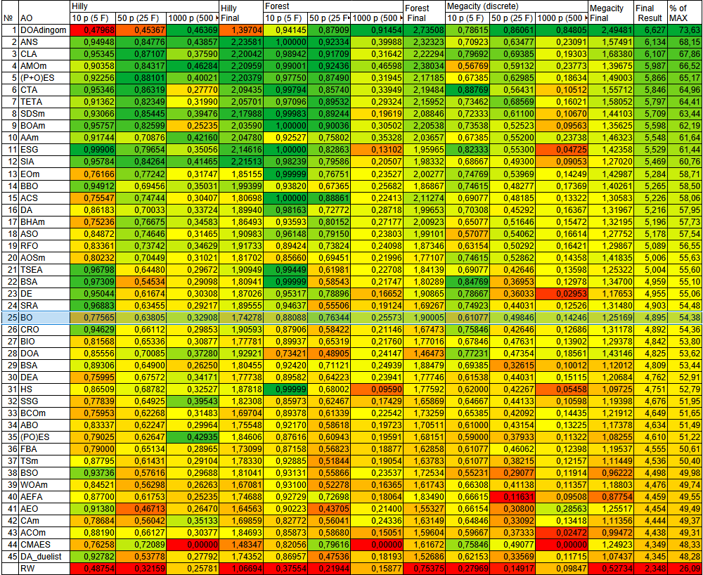
Figure 2. Color gradation of algorithms for the corresponding tests
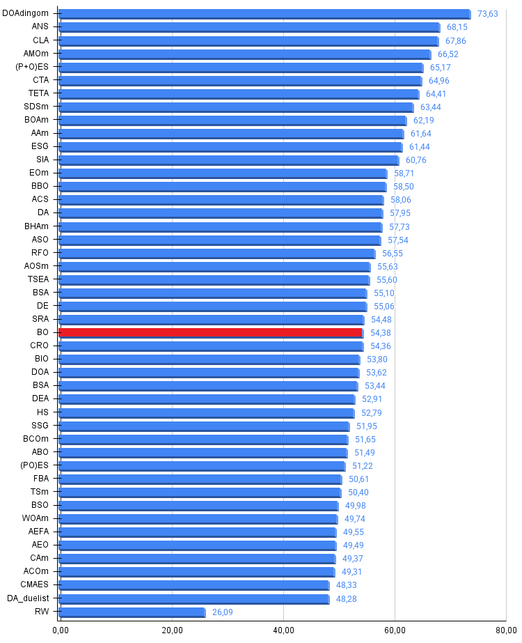
Figure 3. Histogram of the algorithm test results (on a scale from 0 to 100; the higher the score, the better, where 100 is the maximum possible theoretical result; the archive contains a script for calculating the ranking table)
Pros and cons of the BO algorithm:
Pros:
- Effective for medium- and high-dimensional problems.
Cons:
- Requires tuning of many parameters.
- May stagnate on low-dimensional functions.
An archive containing the up-to-date versions of the algorithm code is attached to the article. The author of this article is not responsible for the absolute accuracy of the descriptions of canonical algorithms; changes have been made to many of them to improve search capabilities. The conclusions and judgments presented in the articles are based on the results of the experiments conducted.
Software used in this article
| # | Name | Type | Description |
|---|---|---|---|
| 1 | #C_AO.mqh | Include file | Parent class for population-based optimization algorithms |
| 2 | #C_AO_enum.mqh | Include file | Enumeration of population-based optimization algorithms |
| 3 | TestFunctions.mqh | Include file | Test function library |
| 4 | TestStandFunctions.mqh | Include file | Test bench function library |
| 5 | Utilities.mqh | Include file | Utility function library |
| 6 | CalculationTestResults.mqh | Include file | Script for calculating results for the comparison table |
| 7 | Testing AOs.mq5 | Script | A unified test bench for all population-based optimization algorithms |
| 8 | Simple use of population optimization algorithms.mq5 | Script | A simple example of using population-based optimization algorithms without visualization |
| 9 | Test_AO_BO.mq5 | Script | Test bench for BO |
Translated from Russian by MetaQuotes Ltd.
Original article: https://www.mql5.com/ru/articles/20245
Warning: All rights to these materials are reserved by MetaQuotes Ltd. Copying or reprinting of these materials in whole or in part is prohibited.
This article was written by a user of the site and reflects their personal views. MetaQuotes Ltd is not responsible for the accuracy of the information presented, nor for any consequences resulting from the use of the solutions, strategies or recommendations described.

 Neural Networks in Trading: Adaptive Periodic Segmentation (Conclusion)
 Low-Frequency Quantitative Strategies in MetaTrader 5 (Part 5): Pre-Backtest Evaluation of Machine-Learning-Generated Signals Through Formulaic Alphas
 Feature Engineering for ML (Part 13): Trend-Scanning Features in Python
 Building a Crosshair Volume Profile Indicator in MQL5

- Free trading apps
- Over 8,000 signals for copying
- Economic news for exploring financial markets
You agree to website policy and terms of use