Dendritic Cell Algorithm (DCA)

Contents

1. Introduction
2. Algorithm Implementation
3. Test Results
4. Conclusions

Introduction

Continuing with the topic of optimization inspired by the human immune system, let’s examine the Dendritic Cell Algorithm, DCA — a metaheuristic method inspired by the mechanisms of innate immunity. The original version was developed by Greensmith, Aickelin, and Cayzer in 2005 for anomaly detection in computer systems.

In biology, dendritic cells act as the immune system’s “border guards”: they collect signals from the environment, accumulate information over a certain period of time, and then migrate to the lymph node, where they present the collected data to T lymphocytes. A key feature is that the cell does not make instantaneous decisions but instead integrates a multitude of signals over time, which ensures robustness against noise and random fluctuations.

In the context of optimization, DCA is interpreted differently: a high fitness value is treated as “danger” (a good area for exploitation), while a low fitness value is interpreted as “safety” (an area for exploration or leaving the region). Each agent in the population receives an MCAV (Mature Context Antigen Value) value, which is accumulated based on the results of dendritic cell migrations and determines the movement strategy: local mutation for promising positions and global search for unpromising ones.

Algorithm Implementation

Dendritic cells in the immune system patrol the body's tissues, gathering signals from their surroundings. Once a cell has gathered enough data, it migrates to a lymph node and “reports” what it has detected — danger or normal conditions. Accordingly, the dendritic cell perceives four types of signals:

• PAMP (Pathogen-Associated Molecular Pattern) — a clear danger signal. In biology, these are molecules found only in pathogens; in optimization, they are an indicator of a very good position.
• Danger — a potential danger signal. It indicates damage or stress, but is not an absolute indicator of a threat. In optimization, this is a position that is better than average.
• Safe — a normal-state signal. It indicates a healthy, normal situation; in optimization, it indicates a position that is worse than average.
• Inflammation — a modulatory signal. Enhances the perception of the other signals. In optimization, this refers to the spread of values within a population.

How does signal processing work? The cell converts the input signals into three output signals:

• CSM (Costimulatory Molecule) — the cell’s “life counter.” All signals increase CSM, but with different weights. When CSM reaches the threshold, the cell migrates.
• Semi-mature output — the accumulated “normal-state” signal. It increases only in response to Safe signals.
• Mature output — the accumulated “danger” signal. It increases in response to “PAMP” and “Danger,” and decreases in response to “Safe.”

Processing formula:

Output = (PAMP × Wp + Danger × Wd + Safe × Ws) × (1 + Inflammation)

Inflammation acts as a multiplier — it amplifies all signals proportionally.

Migration and Context. Each cell has its own migration threshold. This is critically important: different thresholds create time windows of varying lengths. Imagine three analysts studying the stock market. The first makes a decision after an hour of observation, the second after a day, and the third after a week. They will see different patterns and draw different conclusions. Combining their opinions is more reliable than relying on a single opinion.

When CSM reaches the threshold, the cell migrates and determines the context:

if semi > mature → context = 0 (normal)

if mature ≥ semi → context = 1 (anomaly)

In optimization, context = 1 means “good position,” and context = 0 means “bad position.”

MCAV (Mature Context Antigen Value) — collective memory. Each agent (a point in the search space) accumulates statistics based on the migration results of the cells that observed it:

MCAV = number of migrations with context 1 / total number of migrations

MCAV close to 1 → the agent is consistently rated as “good”; MCAV close to 0 → the agent is consistently rated as “bad”; MCAV around 0.5 → uncertainty; more data is needed. Consider the example of a restaurant rating based on reviews. A single review is unreliable. One hundred reviews with an average rating of 4.8 are already a strong indication of this establishment’s quality.

Exponential decay. Old data is gradually “forgotten”:

matureSum = matureSum × decay

totalSum = totalSum × decay

With decay = 0.85, two-week-old information carries about 10% of the weight of fresh information. Why is this necessary? Imagine that a restaurant has changed its chef. The old reviews are no longer relevant. The system must adapt to the new reality rather than cling to outdated data.

Movement strategy. Based on the MCAV, the agent selects a strategy:

MCAV > 0.5 (good position) → local mutation. A small random offset for fine-tuning. You have found a good restaurant. It makes sense to try visiting other nearby establishments under the same owner, rather than driving to the other side of town.

MCAV ≤ 0.5 (poor position) → two options:

• with probability (1 - explorationRate) — move toward the best-known solution,
• with probability explorationRate — full reinitialization at a random point.

The restaurant turned out to be terrible. Either you go to a tried-and-tested place (toward the best solution), or you take a risk and try something completely new (reinitialization).

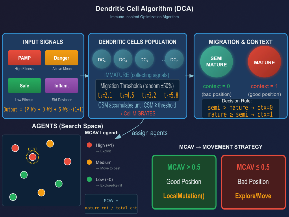
Figure 1. Process Diagram of the DCA Algorithm

The illustration shows:

• INPUT SIGNALS — four input signals (PAMP, Danger, Safe, Inflammation) with their interpretation for optimization
• DENDRITIC CELLS POPULATION — a population of immature cells with different migration thresholds
• MIGRATION & CONTEXT — the migration process and context definition (semi-mature vs. mature)
• AGENTS — agents in the search space, color-coded according to MCAV
• MCAV → MOVEMENT STRATEGY — how the MCAV value determines the movement strategy

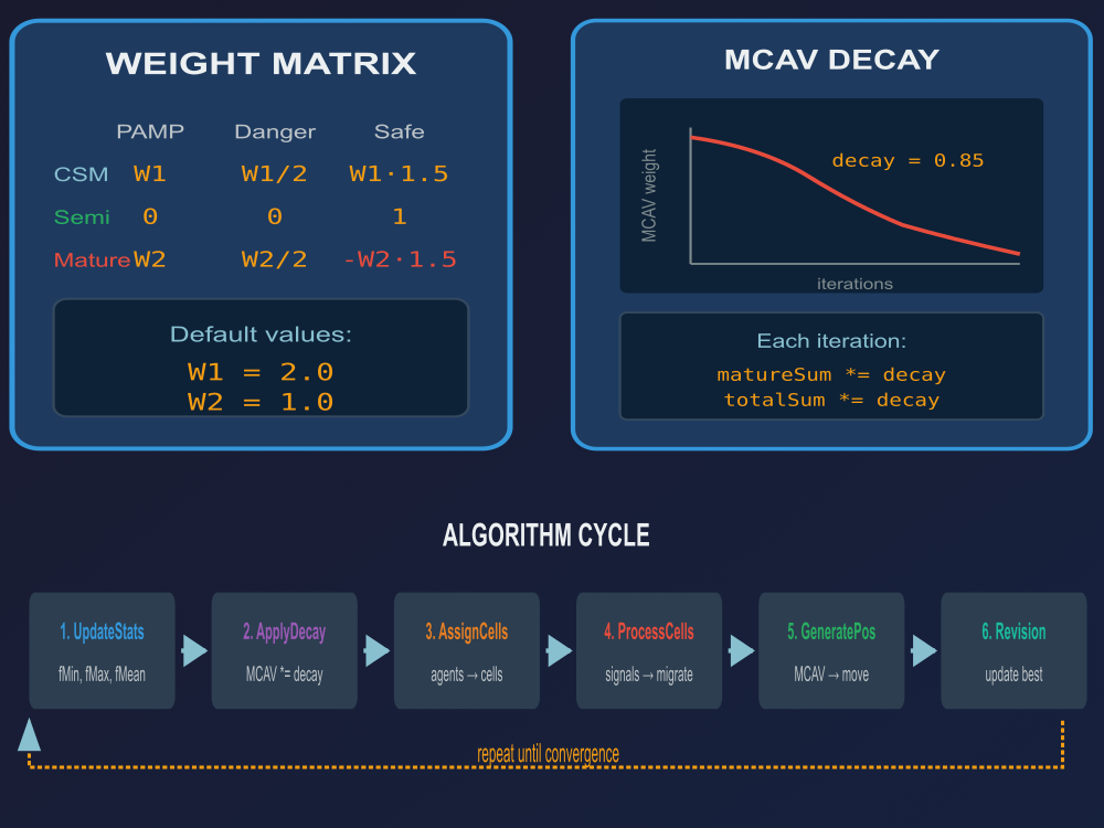
Figure 2. Weight Matrix, Exponential Decay, and the DCA Algorithm Cycle

WEIGHT MATRIX — a weight matrix for signal transformation; MCAV DECAY — exponential decay for "forgetting" old data; ALGORITHM CYCLE — the complete algorithm cycle, step by step.

Now let's move on to writing the pseudocode for the algorithm:

CREATE a population of agents:
For each agent:
- Place it at a random point in the search space
- Compute the fitness at this point
- Set MCAV = 0.5 (neutral value)
- Zero out the migration counters (matureSum = 0, totalSum = 0)

CREATE a population of dendritic cells:
For each cell:
- Set the state to "immature"
- Zero out the signal accumulators (csm = 0, semi = 0, mature = 0)
- Assign a random migration threshold in the range
from (base_threshold × 0.5) to (base_threshold × 1.5)
- Clear the list of observed agents

STORE the best solution found so far

REPEAT until the fitness evaluation limit is reached:

STEP 1. Save the current state
For each agent:
- Store the current position as the previous one
- Store the current fitness as the previous one

STEP 2. Update the population statistics
- Find the minimum fitness value among all agents
- Find the maximum fitness value among all agents
- Calculate the average fitness value of the population

STEP 3. Apply memory decay:
For each agent:
- Multiply matureSum by the decay coefficient
- Multiply totalSum by the decay coefficient
- Recalculate MCAV = matureSum / totalSum
(if totalSum is close to zero, set MCAV = 0.5)

STEP 4. Distribute agents among cells
- Shuffle the list of agents randomly
- Distribute agents evenly among cells
(each cell receives approximately the same number)

STEP 5. Process each cell:
For each dendritic cell:

IF the cell is immature:
For each assigned agent:

GET input signals:
- PAMP = how much the fitness is above the minimum
(normalized from 0 to 1)
- Safe = how much the fitness is below the maximum
(normalized from 0 to 1)
- Danger = 1 if fitness is above average, otherwise 0
- Inflammation = standard deviation of fitness values
in the population (normalized)

CALCULATE output signals:
- modifier = 1 + Inflammation
- csm += (PAMP×2 + Danger×1 + Safe×3) × modifier
- semi += (Safe×1) × modifier
- mature += (PAMP×1 + Danger×0.5 - Safe×1.5) × modifier

CHECK migration condition:
IF csm >= migration threshold:
PERFORM cell migration

STEP 6. Generate new positions
For each agent:

IF MCAV > 0.5 (good position):
- Apply local mutation:
new_position = current + random_offset
(the offset is proportional to the size of the search space
and the mutation coefficient)

ELSE (bad position):
- Generate a random number between 0 and 1

IF the number < exploration_probability:
- Move to a random point in the search space

ELSE:
- Move toward the best-known solution:
new_position = current +
random_step × (best_position - current)

STEP 7. Apply bounds
For each agent:
- If the position moves outside the bounds, reflect it back

STEP 8. Calculate the fitness
For each agent:
- Calculate the fitness at the new position

STEP 9. Update the best solution
For each agent:
IF the new fitness is better than the previous one:
- Accept the new position
ELSE:
- Revert to the previous position

IF the agent’s fitness is better than the global best fitness:
- Update the global best solution

RETURN the best solution found

Now we can proceed to the implementation. The E_DC_State enumeration defines three possible states of a dendritic cell in accordance with the biological model. During the algorithm's operation, a cell starts in the DC_IMMATURE state while accumulating signals, and when it reaches the migration threshold, it transitions to one of two final states. After migration, the cell is reset to DC_IMMATURE for the next observation cycle.

//————————————————————————————————————————————————————————————————————
enum E_DC_State
{
  DC_IMMATURE,
  DC_SEMI_MATURE,
  DC_MATURE
};

//————————————————————————————————————————————————————————————————————

The S_SignalWeights structure stores the weights used to convert the three input signals (PAMP, Danger, Safe) into a single output signal. The algorithm uses three instances of this structure — one for each output signal (CSM, Semi, Mature). This provides a compact way to represent the 3×3 weight matrix from the original article.

//————————————————————————————————————————————————————————————————————
struct S_SignalWeights
{
    double wPAMP;
    double wDanger;
    double wSafe;
};

//————————————————————————————————————————————————————————————————————

The S_DCA_Cell structure represents a single dendritic cell with all of its attributes:

• State: cells can be immature or mature (state).
• Cell metrics: the cell has metrics (csm, semi, mature) that influence whether agents will move to this cell.
• Migration threshold: defines the conditions under which agents can leave this cell (threshold).
• Capacity: each cell has a limited number of slots for agents (agentIndices, agentCount, maxAgents from Init).

The structure also provides methods for:

• Init — sets the initial state, zeroes the signal accumulators, and allocates memory for the array of agent indices.
• Reset — resets the cell and updates its threshold. The key point is that a new migration threshold is generated randomly with each reset. This creates a variety of observation time windows across cells.
• AddAgent — adds an agent to the cell's list if there is room. A simple operation with an array-bounds check. Agents are distributed evenly across the cells at each iteration.

//————————————————————————————————————————————————————————————————————
struct S_DCA_Cell
{
    E_DC_State state;
    double     csm;
    double     semi;
    double     mature;
    double     threshold;
    int        agentIndices [];
    int        agentCount;

    void Init (double migrationThreshold, int maxAgents)
    {
      state      = DC_IMMATURE;
      csm        = 0.0;
      semi       = 0.0;
      mature     = 0.0;
      threshold  = migrationThreshold;
      agentCount = 0;
      ArrayResize (agentIndices, maxAgents);
    }

    void Reset (double newThreshold)
    {
      state      = DC_IMMATURE;
      csm        = 0.0;
      semi       = 0.0;
      mature     = 0.0;
      threshold  = newThreshold;
      agentCount = 0;
    }

    void AddAgent (int idx)
    {
      if (agentCount < ArraySize (agentIndices))
      {
        agentIndices [agentCount++] = idx;
      }
    }
};

//————————————————————————————————————————————————————————————————————

The S_MCAV structure stores context statistics for a single agent. The Init method sets the initial state. An initial value of 0.5 indicates uncertainty — the agent has not yet accumulated statistics. The AddContext method adds the result of a cell migration.

The "ctx" parameter takes the value 0 (bad position) or 1 (good position). When ctx = 1, both counters are incremented; when ctx = 0, only the total counter is incremented. The ApplyDecay method applies exponential decay. When rate = 0.85, information from ten iterations ago has about 20% of the weight of fresh information. This allows the algorithm to adapt to changes in the fitness landscape.

The Update method recalculates the MCAV value. Division-by-zero protection — if there are insufficient statistics, a neutral value is returned.

//————————————————————————————————————————————————————————————————————
struct S_MCAV
{
    double matureSum;
    double totalSum;
    double value;

    void Init ()
    {
      matureSum = 0.0;
      totalSum  = 0.0;
      value     = 0.5;
    }

    void AddContext (int ctx)
    {
      totalSum += 1.0;
      if (ctx == 1) matureSum += 1.0;
    }

    void ApplyDecay (double rate)
    {
      matureSum *= rate;
      totalSum  *= rate;
    }

    void Update ()
    {
      if (totalSum > 0.01) value = matureSum / totalSum;
      else value = 0.5;
    }
};

//————————————————————————————————————————————————————————————————————

The C_AO_DCA class is an implementation of the Dendritic Cell Algorithm (DCA). It mimics the operation of the immune system by using the concept of dendritic cells to detect threats and make decisions, and inherits from the base class "C_AO".

SetParams — the method loads values from the "params" array into the corresponding class variables. After being loaded, all parameters go through a series of checks to ensure that they are within acceptable limits. These constraints prevent invalid configurations: a minimum of 4 agents, a minimum of 2 cells, and a decay value within reasonable limits. Init is the key initialization function for the DCA. The base threshold "tMedian" is calculated as half of the maximum possible "CSM" in a single iteration and is then multiplied by "lifespanMult". This ensures that, on average, cells live for several iterations before migrating.

Moving is the main method that, in a single cycle (or “step”) of the DCA, processes each agent, obtains input signals, updates cell states (ProcessCell), processes cells, handles cell migration events, applies mutations, generates new positions, updates statistics, and applies decay.

Revision is the method used to retrieve the best solution found by the algorithm.

Private methods:

• InitWeights — initializes the weights for the signals;
• GetMigrationThreshold — calculates and returns the migration threshold;
• CalcOutputSignals — calculates the output signals (outCSM, outSemi, outMature) for a cell based on the input signals (pamp, danger, safe, infl) and the weights "wCSM," "wSemi," and "wMature";
• GetInputSignals — retrieves the input signals for a specific agent (idx);
• UpdatePopStats — updates the population statistics (fMinPop, fMaxPop, fMeanPop);
• AssignAgentsToCells — distributes agents evenly among cells;
• ProcessCell — processes the state and contents of a single specific cell;
• MigrateCell — implements cell migration logic, assigns context to observed agents, and resets the cell;
• GeneratePosition — generates a new position (solution) for agent "idx";
• LocalMutation — applies a mutation to an agent, changing its position;
• MoveTowardsBest — moves the agent toward the best solution found, taking strength into account;
• GlobalReinit — performs a global reinitialization of the agent;
• ApplyBounds — ensures that the agent's position is within the valid bounds.

//————————————————————————————————————————————————————————————————————
class C_AO_DCA : public C_AO
{
  public: //----------------------------------------------------------
  ~C_AO_DCA () { }

  C_AO_DCA ()
  {
    ao_name = "DCA";
    ao_desc = "Dendritic Cell Algorithm";
    ao_link = "https://www.mql5.com/en/articles/20479";

    popSize         = 50;
    numCells        = 10;
    lifespanMult    = 5.0;
    decayRate       = 0.85;
    mutationRate    = 0.1;
    explorationRate = 0.3;

    ArrayResize (params, 6);
    params [0].name = "popSize";          params [0].val = popSize;
    params [1].name = "numCells";         params [1].val = numCells;
    params [2].name = "lifespanMult";     params [2].val = lifespanMult;
    params [3].name = "decayRate";        params [3].val = decayRate;
    params [4].name = "mutationRate";     params [4].val = mutationRate;
    params [5].name = "explorationRate";  params [5].val = explorationRate;
  }

  void SetParams ()
  {
    popSize         = (int)params [0].val;
    numCells        = (int)params [1].val;
    lifespanMult    = params      [2].val;
    decayRate       = params      [3].val;
    mutationRate    = params      [4].val;
    explorationRate = params      [5].val;

    if (popSize < 4) popSize = 4;
    if (numCells < 2) numCells = 2;
    if (numCells > popSize) numCells = popSize;
    if (lifespanMult < 1.0) lifespanMult = 1.0;
    if (decayRate < 0.5) decayRate = 0.5;
    if (decayRate > 0.99) decayRate = 0.99;
    if (mutationRate < 0.001) mutationRate = 0.001;
    if (mutationRate > 1.0) mutationRate = 1.0;
    if (explorationRate < 0.0) explorationRate = 0.0;
    if (explorationRate > 1.0) explorationRate = 1.0;
  }

  bool Init (const double &rangeMinP  [],
             const double &rangeMaxP  [],
             const double &rangeStepP [],
             const int     epochsP);

  void Moving   ();
  void Revision ();

  //------------------------------------------------------------------
  int    numCells;
  double lifespanMult;
  double decayRate;
  double mutationRate;
  double explorationRate;

  private: //---------------------------------------------------------
  S_DCA_Cell      cells [];
  S_MCAV          mcav  [];
  S_SignalWeights wCSM;
  S_SignalWeights wSemi;
  S_SignalWeights wMature;

  double tMedian;
  double fMinPop;
  double fMaxPop;
  double fMeanPop;

  void   InitWeights           ();
  double GetMigrationThreshold ();
  void   CalcOutputSignals     (double pamp, double danger, double safe, double infl,
                                double &outCSM, double &outSemi, double &outMature);
  void   GetInputSignals       (int idx, double &pamp, double &danger, double &safe, double &infl);
  void   UpdatePopStats        ();
  void   AssignAgentsToCells   ();
  void   ProcessCell           (int cellIdx);
  void   MigrateCell           (int cellIdx);
  void   GeneratePosition      (int idx);
  void   LocalMutation         (int idx);
  void   MoveTowardsBest       (int idx, double strength);
  void   GlobalReinit          (int idx);
  void   ApplyBounds           (int idx);
};
//————————————————————————————————————————————————————————————————————

The Init initialization function for the Dendritic Cell Algorithm C_AO_DCA. It performs the initial setup before running the main algorithm.

First, the standard initialization function StandardInit is called, which prepares the necessary data structures and parameters common to all algorithms by passing the input value ranges (rangeMinP, rangeMaxP, rangeStepP) and the number of epochs (epochsP). If this basic initialization fails, the Init function also terminates with an error.

The private method InitWeights is called; it sets the initial values for the weight coefficients used in the algorithm.

Calculating the median lifespan. First, the maximum value for the CSM signals is calculated (csmMax). This is done by summing all the weight coefficients associated with the corresponding input signals (PAMP, Danger, Safe) from the wCSM structure. Next, "tMedian" (the median lifespan) is calculated. This value is calculated as half of "csmMax" multiplied by "ifespanMult" (the lifespan multiplier).

Cell initialization. Memory is allocated for the "cells" array (which represents dendritic cells) based on the value of "numCells" (the number of cells). The maximum number of agents that can be placed in each cell is calculated. This is done by dividing the total number of agents by the number of cells and adding a small buffer (plus 2) as a margin for uneven distribution.

The loop iterates through each cell and calls the Init method. In this process, the cell is passed the migration threshold obtained using GetMigrationThreshold and the maximum number of agents it can accommodate.

Agent initialization. Memory is allocated for the "mcav" array. The loop iterates over each agent. The Init method is called for each agent to perform the initial setup.

The Init function prepares the environment for the Dendritic Cell Algorithm to run by configuring the dendritic cells, distributing them, initializing the agent population, and calculating certain key parameters.

//————————————————————————————————————————————————————————————————————
bool C_AO_DCA::Init (const double &rangeMinP  [],
                     const double &rangeMaxP  [],
                     const double &rangeStepP [],
                     const int     epochsP)
{
  if (!StandardInit (rangeMinP, rangeMaxP, rangeStepP)) return false;

  //------------------------------------------------------------------
  InitWeights ();

  double csmMax = wCSM.wPAMP + wCSM.wDanger + wCSM.wSafe;
  tMedian = 0.5 * csmMax * lifespanMult;

  ArrayResize (cells, numCells);
  int maxAgentsPerCell = (popSize / numCells) + 2;

  for (int i = 0; i < numCells; i++)
  {
    cells [i].Init (GetMigrationThreshold (), maxAgentsPerCell);
  }

  ArrayResize (mcav, popSize);
  for (int i = 0; i < popSize; i++)
  {
    mcav [i].Init ();
  }

  return true;
}
//————————————————————————————————————————————————————————————————————

The InitWeights function stores the weights used to convert the three input signals (PAMP, Danger, Safe) into a single output signal. The algorithm uses three instances of this structure — one for each output signal (CSM, Semi, Mature). This allows for a compact representation of a 3×3 weight matrix.

//————————————————————————————————————————————————————————————————————
void C_AO_DCA::InitWeights ()
{
  double W1 = 2.0;
  double W2 = 1.0;

  wCSM.wPAMP   = W1;
  wCSM.wDanger = W1 / 2.0;
  wCSM.wSafe   = W1 * 1.5;

  wSemi.wPAMP   = 0.0;
  wSemi.wDanger = 0.0;
  wSemi.wSafe   = 1.0;

  wMature.wPAMP   = W2;
  wMature.wDanger = W2 / 2.0;
  wMature.wSafe   = -W2 * 1.5;
}
//————————————————————————————————————————————————————————————————————

The GetMigrationThreshold method returns a random migration threshold value that ranges from 50% to 150% of the base value "tMedian". This approach introduces stochasticity (randomness) into the migration decision-making process, which is often used to model biological processes where behavior is not always deterministic.

//————————————————————————————————————————————————————————————————————
double C_AO_DCA::GetMigrationThreshold ()
{
  return u.RNDfromCI (tMedian * 0.5, tMedian * 1.5);
}
//————————————————————————————————————————————————————————————————————

The CalcOutputSignals method takes the levels of various signals and the inflammation coefficient as input, applies weights corresponding to three different states and processing paths (CSM, Semi, Mature), and then scales the result by a common factor that depends on the inflammation level. Finally, any negative results are clipped to zero.

//————————————————————————————————————————————————————————————————————
void C_AO_DCA::CalcOutputSignals (double pamp, double danger, double safe, double infl,
                                  double &outCSM, double &outSemi, double &outMature)
{
  double amp = 1.0 + infl;

  outCSM    = (pamp * wCSM.wPAMP    + danger * wCSM.wDanger    + safe * wCSM.wSafe) * amp;
  outSemi   = (pamp * wSemi.wPAMP   + danger * wSemi.wDanger   + safe * wSemi.wSafe) * amp;
  outMature = (pamp * wMature.wPAMP + danger * wMature.wDanger + safe * wMature.wSafe) * amp;

  if (outCSM < 0.0) outCSM    = 0.0;
  if (outSemi < 0.0) outSemi   = 0.0;
  if (outMature < 0.0) outMature = 0.0;
}
//————————————————————————————————————————————————————————————————————

The UpdatePopStats method iterates through the entire population, ignoring inactive elements (marked with the value -DBL_MAX), and calculates the minimum, maximum, and average values for all active elements. If there are no active elements, predefined default values (0, 0.5, 1.0) are set for these statistics. This method is likely called periodically to monitor and analyze the state of the entire population of dendritic cells.

//————————————————————————————————————————————————————————————————————
void C_AO_DCA::UpdatePopStats ()
{
  fMinPop  =  DBL_MAX;
  fMaxPop  = -DBL_MAX;
  fMeanPop =  0.0;
  int cnt  =  0;

  for (int i = 0; i < popSize; i++)
  {
    if (a [i].f != -DBL_MAX)
    {
      if (a [i].f > fMaxPop) fMaxPop = a [i].f;
      if (a [i].f < fMinPop) fMinPop = a [i].f;
      fMeanPop += a [i].f;
      cnt++;
    }
  }

  if (cnt > 0)
  {
    fMeanPop /= cnt;
  }
  else
  {
    fMaxPop  = 1.0;
    fMinPop  = 0.0;
    fMeanPop = 0.5;
  }
}
//————————————————————————————————————————————————————————————————————

The GetInputSignals method converts an individual fitness value into a set of signals (pamp, danger, safe, infl) that will be used by other parts of the model:

• pamp — reflects an element's position in the population on the "f" scale (a high f value corresponds to a high pamp value)
• danger — increases when an element's "f" value significantly exceeds the population average
• safe — has a higher value when the element's fitness is below the population average
• infl — reflects the overall "activation" or "heterogeneity" of the population, based on the dispersion of fitness values; a high spread within the population indicates high "Inflammation".

This logic allows individual cells (or agents) to obtain information not only about their own state, but also about the state of the entire population.

//————————————————————————————————————————————————————————————————————
void C_AO_DCA::GetInputSignals (int idx, double &pamp, double &danger, double &safe, double &infl)
{
  double f = a [idx].f;

  pamp   = 0.5;
  danger = 0.0;
  safe   = 0.5;
  infl   = 0.0;

  if (f == -DBL_MAX) return;

  double range = fMaxPop - fMinPop;
  if (range < 1e-10) return;

  double fNorm = (f - fMinPop) / range;
  fNorm = MathMax (0.0, MathMin (1.0, fNorm));

  pamp = fNorm;

  if (f > fMeanPop)
  {
    danger = (f - fMeanPop) / range;
    danger = MathMin (danger * 2.0, 1.0);
  }

  safe = 1.0 - fNorm;

  if (f < fMeanPop)
  {
    double belowMean = (fMeanPop - f) / range;
    safe = MathMin (safe + belowMean, 1.0);
  }

  double variance = 0.0;
  int    cnt      = 0;

  for (int i = 0; i < popSize; i++)
  {
    if (a [i].f != -DBL_MAX)
    {
      variance += (a [i].f - fMeanPop) * (a [i].f - fMeanPop);
      cnt++;
    }
  }

  if (cnt > 1)
  {
    double stdDev = MathSqrt (variance / cnt);
    infl = MathMin (stdDev / range, 1.0);
  }
}
//————————————————————————————————————————————————————————————————————

This method performs a uniform cyclic distribution of all agents in the population across a specified number of cells. With 50 agents and 10 cells, each cell receives exactly 5 agents. This ensures an even load on all cells.

//————————————————————————————————————————————————————————————————————
void C_AO_DCA::AssignAgentsToCells ()
{
  for (int c = 0; c < numCells; c++)
  {
    cells [c].agentCount = 0;
  }

  for (int i = 0; i < popSize; i++)
  {
    int cellIdx = i % numCells;
    cells [cellIdx].AddAgent (i);
  }
}
//————————————————————————————————————————————————————————————————————

The Moving method simulates the following in a single step:

1. Saves the agents' states before changes are made.
2. Updates the overall "environment" or population statistics.
3. Applies general effects (decay).
4. Organizes agents (distributes them among cells).
5. Performs local interactions and computations (cell processing).
6. Updates the auxiliary structures (mcav).
7. Determines a new location for each agent based on its state, interactions, and global factors.
8. Keeps agents within the specified bounds.

This method is the "core" of the evolutionary process, in which the population's behavior changes and adapts over time. The method implements the full iteration cycle of the algorithm. Saving the previous positions is necessary for greedy selection in the Revision method.

//————————————————————————————————————————————————————————————————————
void C_AO_DCA::Moving ()
{
  if (!revision)
  {
    for (int i = 0; i < popSize; i++)
    {
      for (int c = 0; c < coords; c++)
      {
        a [i].c [c] = u.RNDfromCI (rangeMin [c], rangeMax [c]);
        a [i].c [c] = u.SeInDiSp (a [i].c [c], rangeMin [c], rangeMax [c], rangeStep [c]);
      }
    }

    revision = true;
    return;
  }

  //------------------------------------------------------------------
  for (int i = 0; i < popSize; i++)
  {
    ArrayCopy (a [i].cP, a [i].c, 0, 0, coords);
    a [i].fP = a [i].f;
  }

  UpdatePopStats ();

  for (int i = 0; i < popSize; i++)
  {
    mcav [i].ApplyDecay (decayRate);
  }

  AssignAgentsToCells ();

  for (int c = 0; c < numCells; c++)
  {
    ProcessCell (c);
  }

  for (int i = 0; i < popSize; i++)
  {
    mcav [i].Update ();
  }

  for (int i = 0; i < popSize; i++)
  {
    GeneratePosition (i);
    ApplyBounds (i);
  }
}
//————————————————————————————————————————————————————————————————————

The ProcessCell method performs the following actions:

1. Checks that the cell is immature and contains agents.
2. Iterates through all agents in the cell.
3. Obtains input signals for each agent.
4. Computes the output signals for each agent.
5. Sums the output signals from all agents.
6. Updates the cell's aggregate values based on the sums of the agents' signals.
7. Checks whether the aggregate csm value has reached the threshold.
8. If the threshold is reached, it initiates the migration process from this cell.

This method simulates how the activity of agents within a cell can lead to the "maturation" of the cell itself, preparing it for subsequent stages of agent redistribution.

//————————————————————————————————————————————————————————————————————
void C_AO_DCA::ProcessCell (int cellIdx)
{
  if (cells [cellIdx].state != DC_IMMATURE) return;
  if (cells [cellIdx].agentCount == 0) return;

  double totalCSM    = 0.0;
  double totalSemi   = 0.0;
  double totalMature = 0.0;

  for (int i = 0; i < cells [cellIdx].agentCount; i++)
  {
    int agentIdx = cells [cellIdx].agentIndices [i];

    if (agentIdx < 0 || agentIdx >= popSize) continue;
    if (a [agentIdx].f == -DBL_MAX) continue;

    double pamp, danger, safe, infl;
    GetInputSignals (agentIdx, pamp, danger, safe, infl);

    double outCSM, outSemi, outMature;
    CalcOutputSignals (pamp, danger, safe, infl, outCSM, outSemi, outMature);

    totalCSM    += outCSM;
    totalSemi   += outSemi;
    totalMature += outMature;
  }

  cells [cellIdx].csm    += totalCSM;
  cells [cellIdx].semi   += totalSemi;
  cells [cellIdx].mature += totalMature;

  if (cells [cellIdx].csm >= cells [cellIdx].threshold)
  {
    MigrateCell (cellIdx);
  }
}
//————————————————————————————————————————————————————————————————————

The MigrateCell method performs the following functions:

• Classifies a cell, after it reaches the threshold, as either "semi-mature" or "fully mature," based on the relative contributions of "semi" and "mature."
• Passes information about the cell's new state (context "ctx") to all agents located within it. This allows the agents to adapt to the cell's new stage of development.
• Reinitializes the cell by resetting its accumulated parameters so that it can participate in subsequent "maturation" cycles.

This method is a key component of the model, in which cells can “mature” and pass this information on to their agents, influencing their subsequent behavior and development. If more Safe signals (semi > mature) have accumulated during the cell's lifetime, the positions are evaluated as “bad”. Otherwise, they are evaluated as “good.” All agents observed by this cell receive the same context.

//————————————————————————————————————————————————————————————————————
void C_AO_DCA::MigrateCell (int cellIdx)
{
  int ctx;

  if (cells [cellIdx].semi > cells [cellIdx].mature)
  {
    cells [cellIdx].state = DC_SEMI_MATURE;
    ctx = 0;
  }
  else
  {
    cells [cellIdx].state = DC_MATURE;
    ctx = 1;
  }

  for (int i = 0; i < cells [cellIdx].agentCount; i++)
  {
    int agentIdx = cells [cellIdx].agentIndices [i];
    if (agentIdx >= 0 && agentIdx < popSize)
    {
      mcav [agentIdx].AddContext (ctx);
    }
  }

  cells [cellIdx].Reset (GetMigrationThreshold ());
}
//————————————————————————————————————————————————————————————————————

The GeneratePosition method implements an agent update strategy based on its current "value" (m). For high-value agents (m > 0.5), a local mutation occurs that aims to fine-tune or improve existing good solutions. For low- or medium-value agents (m <= 0.5):

• There is a probability of global reinitialization (GlobalReinit), which depends on the global "explorationRate" and the current "m". This is a radical form of exploration when the current solution is not optimal.
• If no global reinitialization occurs, the agent moves toward the best solution (MoveTowardsBest) with a force proportional to "m". This is directed exploration or exploitation, in which the agent attempts to move toward more promising areas, but less aggressively than in the (m > 0.5) case. The lower the MCAV, the higher the probability of global reinitialization.

//————————————————————————————————————————————————————————————————————
void C_AO_DCA::GeneratePosition (int idx)
{
  double m = mcav [idx].value;

  if (m > 0.5)
  {
    LocalMutation (idx);
  }
  else
  {
    double r = u.RNDfromCI (0.0, 1.0);
    double reinitProb = explorationRate * (1.0 - m * 2.0);
    if (reinitProb < 0.0) reinitProb = 0.0;

    if (r < reinitProb)
    {
      GlobalReinit (idx);
    }
    else
    {
      double strength = 1.0 - m;
      MoveTowardsBest (idx, strength);
    }
  }
}
//————————————————————————————————————————————————————————————————————

The LocalMutation method performs the following: for each dimension (coordinate) of the agent's position, it calculates a random change (delta). This change is proportional to the specified mutation rate (mutationRate), the range of valid values for that coordinate (range), and a random direction factor (from -1 to 1). This random change is applied to the agent's current position along that coordinate.

This process results in small, random deviations from the agent's current position, which is a standard technique for locally exploring the search space. When mutationRate = 0.1, the maximum offset is ±10% of the range for each coordinate. The mutation is applied to the previous position, cP, not to the current one.

//————————————————————————————————————————————————————————————————————
void C_AO_DCA::LocalMutation (int idx)
{
  for (int c = 0; c < coords; c++)
  {
    double range = rangeMax [c] - rangeMin [c];
    double delta = mutationRate * range * u.RNDfromCI (-1.0, 1.0);
    a [idx].c [c] = a [idx].cP [c] + delta;
  }
}
//————————————————————————————————————————————————————————————————————

The MoveTowardsBest method updates the agent's position by combining two components:

1. Moving toward the best global solution: the agent moves toward cB (the best solution). The extent of this movement is controlled by a random number "r," which, in turn, depends on "strength" and randomness. The higher the "strength," the greater the likelihood of moving in the cB direction. The "strength" parameter controls the strength of the attraction: the worse the current position (the lower the MCAV), the more strongly the agent tends toward the best solution.
2. A small point mutation. Adding noise prevents premature convergence.

//————————————————————————————————————————————————————————————————————
void C_AO_DCA::MoveTowardsBest (int idx, double strength)
{
  if (fB == -DBL_MAX)
  {
    LocalMutation (idx);
    return;
  }

  for (int c = 0; c < coords; c++)
  {
    double r     = u.RNDfromCI (0.0, 1.0) * strength;
    double range = rangeMax [c] - rangeMin [c];

    a [idx].c [c] = a [idx].cP [c]
                    + r * (cB [c] - a [idx].cP [c])
                    + mutationRate * range * u.RNDfromCI (-0.5, 0.5);
  }
}
//————————————————————————————————————————————————————————————————————

The GlobalReinit method is intended to fully reinitialize the position of the agent with index "idx". This method is called when a significant event occurs that requires the agent's state to be reset. The global exploration mechanism allows the algorithm to escape from local optima.

//————————————————————————————————————————————————————————————————————
void C_AO_DCA::GlobalReinit (int idx)
{
  for (int c = 0; c < coords; c++)
  {
    a [idx].c [c] = u.RNDfromCI (rangeMin [c], rangeMax [c]);
  }
}
//————————————————————————————————————————————————————————————————————

The ApplyBounds method uses reflection instead of simple clipping — this preserves the movement's "momentum." If the position is still out of bounds after reflection (a major overshoot), random reinitialization is performed.

//————————————————————————————————————————————————————————————————————
void C_AO_DCA::ApplyBounds (int idx)
{
  for (int c = 0; c < coords; c++)
  {
    if (a [idx].c [c] < rangeMin [c])
    {
      a [idx].c [c] = rangeMin [c] + fabs (a [idx].c [c] - rangeMin [c]);
      if (a [idx].c [c] > rangeMax [c]) a [idx].c [c] = u.RNDfromCI (rangeMin [c], rangeMax [c]);
    }

    if (a [idx].c [c] > rangeMax [c])
    {
      a [idx].c [c] = rangeMax [c] - fabs (a [idx].c [c] - rangeMax [c]);
      if (a [idx].c [c] < rangeMin [c]) a [idx].c [c] = u.RNDfromCI (rangeMin [c], rangeMax [c]);
    }

    a [idx].c [c] = u.SeInDiSp (a [idx].c [c], rangeMin [c], rangeMax [c], rangeStep [c]);
  }
}
//————————————————————————————————————————————————————————————————————

The Revision method does the following:

1. Checks the agents' individual best positions: if an agent's current target turns out to be worse than its best recorded position, the agent "returns" to its best position.
2. Finds and updates the absolute global best solution in the population.

As a result, greedy selection is performed and the best solution is updated.

//————————————————————————————————————————————————————————————————————
void C_AO_DCA::Revision ()
{
  for (int i = 0; i < popSize; i++)
  {
    if (a [i].fP != -DBL_MAX && a [i].fP > a [i].f)
    {
      a [i].f = a [i].fP;
      ArrayCopy (a [i].c, a [i].cP, 0, 0, coords);
    }
  }

  for (int i = 0; i < popSize; i++)
  {
    if (a [i].f > fB)
    {
      fB = a [i].f;
      ArrayCopy (cB, a [i].c, 0, 0, coords);
    }
  }
}
//————————————————————————————————————————————————————————————————————

Test Results

DCA|Dendritic Cell Algorithm|50.0|20.0|5.0|0.5|0.01|0.8|
=============================
5 Hilly's; Func runs: 10000; result: 0.8178926955715087
25 Hilly's; Func runs: 10000; result: 0.4463156865164426
500 Hilly's; Func runs: 10000; result: 0.276079330277272
=============================
5 Forest's; Func runs: 10000; result: 0.6916302728114128
25 Forest's; Func runs: 10000; result: 0.3490153259275664
500 Forest's; Func runs: 10000; result: 0.19980310116079952
=============================
5 Megacity's; Func runs: 10000; result: 0.4492307692307693
25 Megacity's; Func runs: 10000; result: 0.22399999999999992
500 Megacity's; Func runs: 10000; result: 0.10461538461538558
=============================
Overall score: 3.55858 (39.54%)

For low-dimensional functions, convergence performance is poor, especially on the discrete Megacity function.

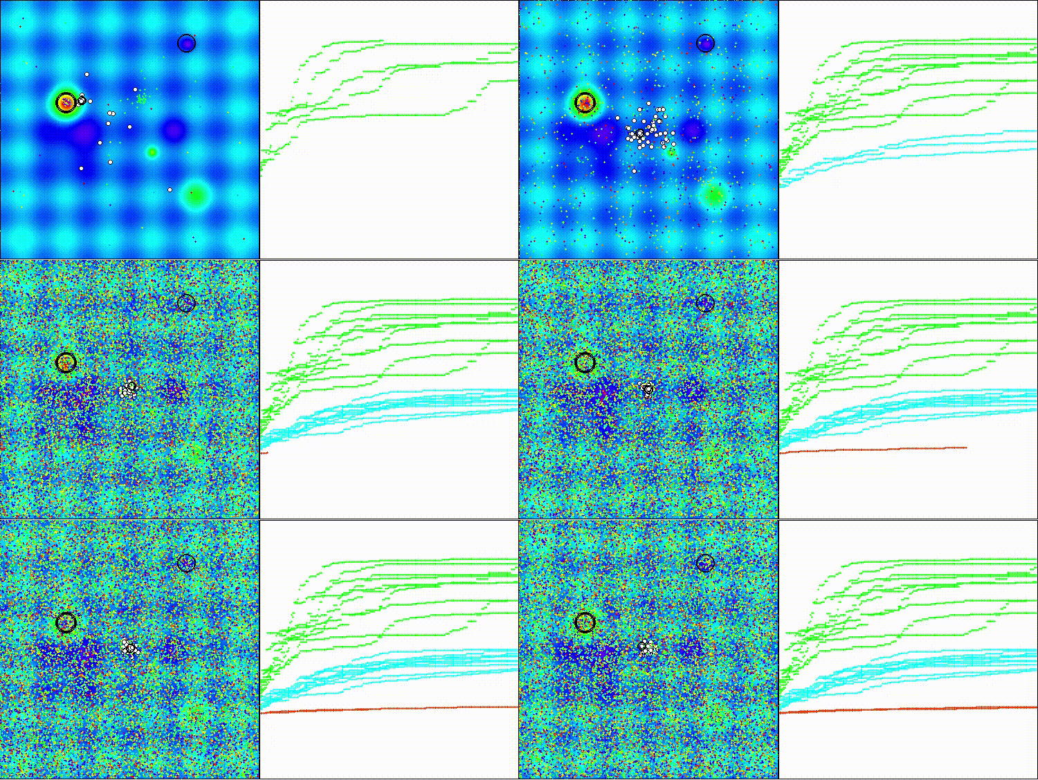
DCA on the Hilly test function

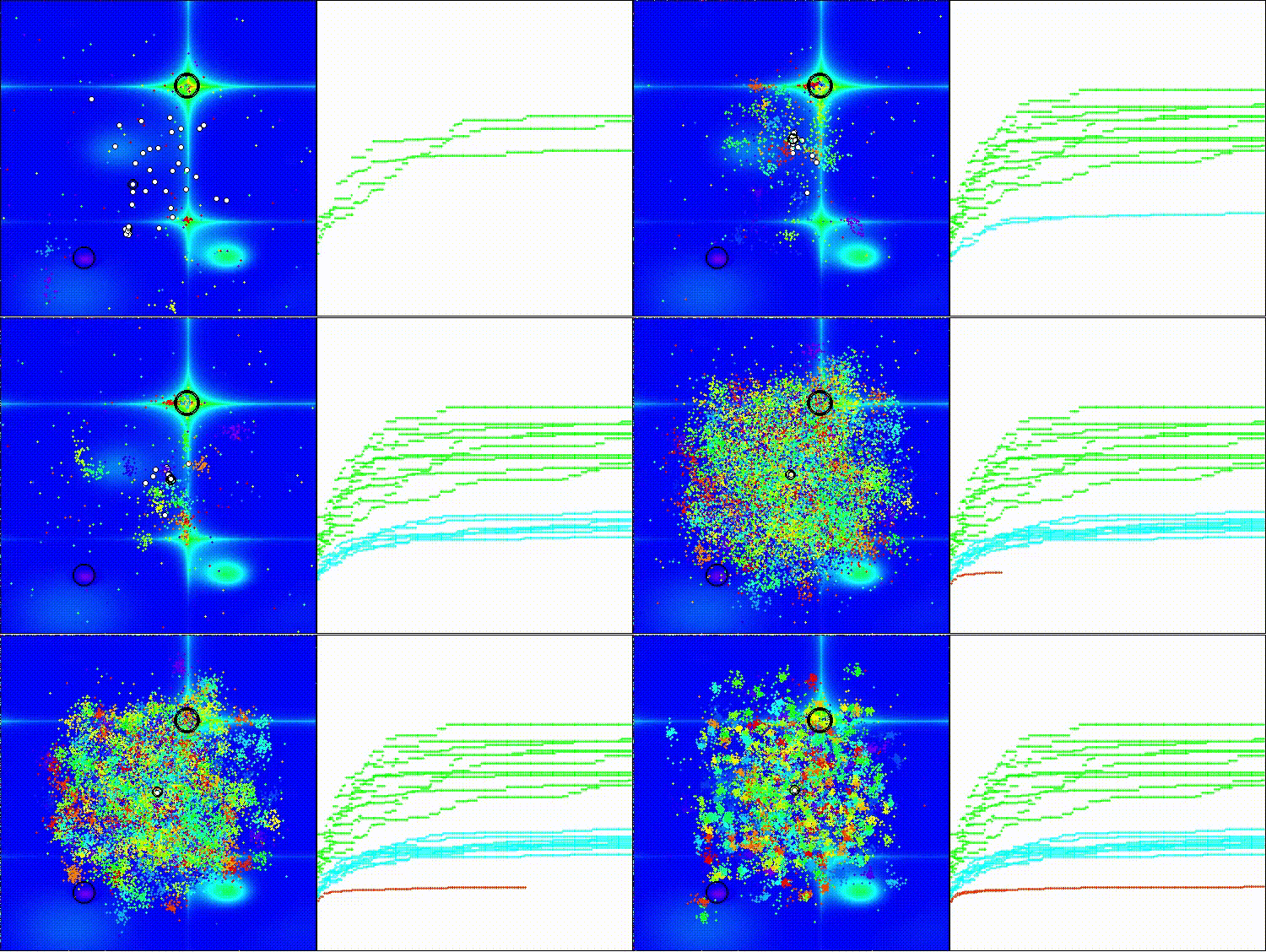
DCA on the Forest test function

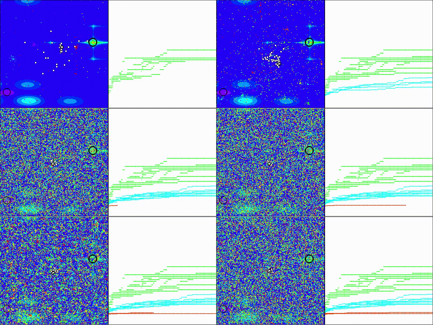
DCA on the Megacity test function

For problems involving benchmark functions, the DCA algorithm performs well; it has no trouble handling simpler functions.

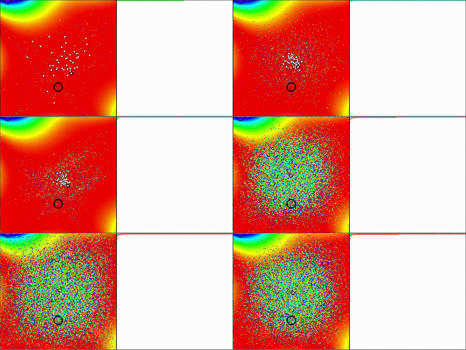
DCA on the benchmark function GoldsteinPrice

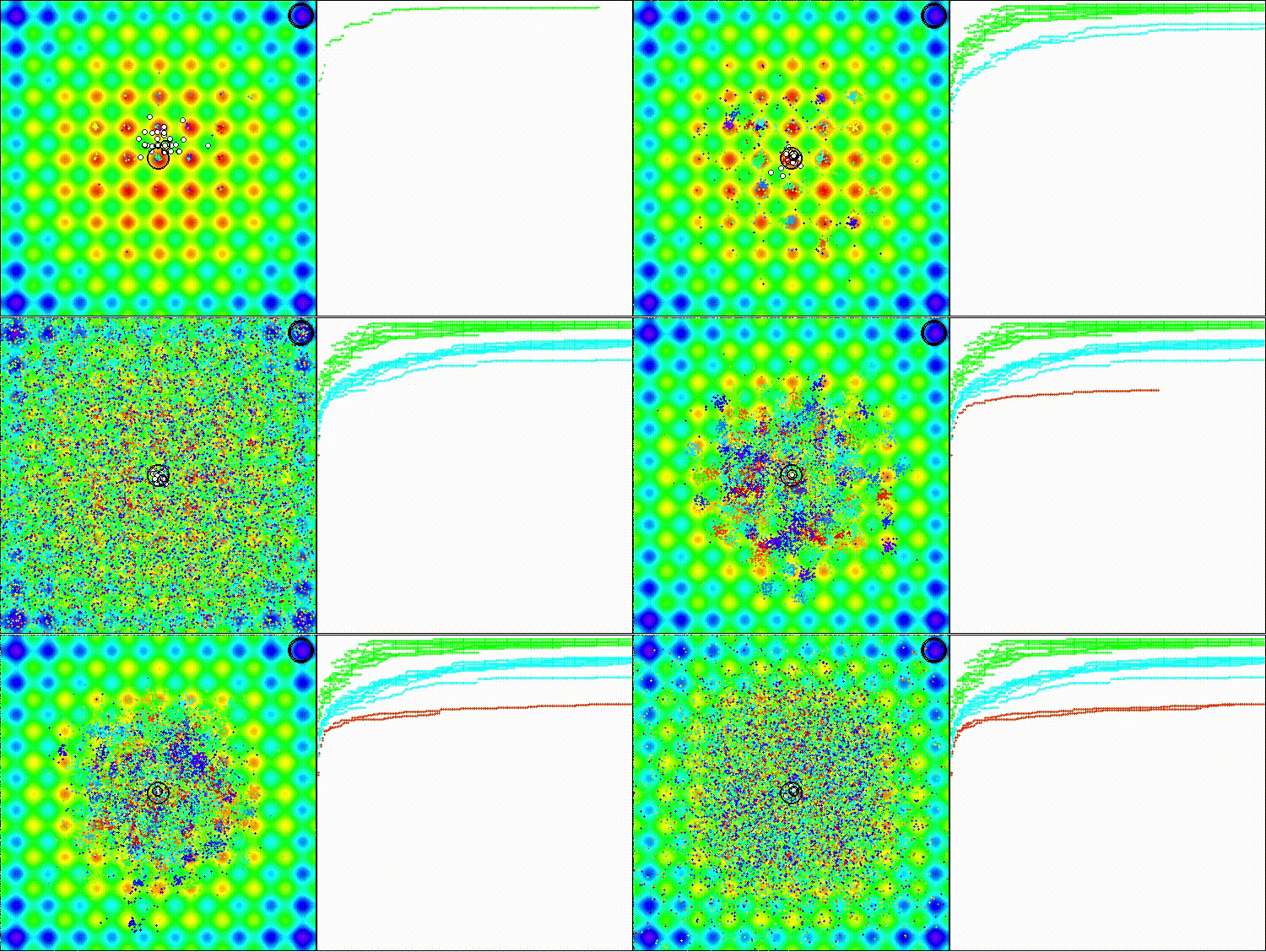
DCA on the benchmark function Rastrigin

In the ranking table of population-based optimization methods, the DCA algorithm is included for informational purposes only.

No.	AO	Description	Hilly			Hilly Final	Forest			Forest Final	Megacity (discrete)			Megacity Final	Final Result	% of MAX
			10 p (5 F)	50 p (25 F)	1000 p (500 F)		10 p (5 F)	50 p (25 F)	1000 p (500 F)		10 p (5 F)	50 p (25 F)	1000 p (500 F)
1	DOAdingom	dingo_optimization_algorithm_M	0.47968	0.45367	0.46369	1.39704	0.94145	0.87909	0.91454	2.73508	0.78615	0.86061	0.84805	2.49481	6.627	73.63
2	ANS	across neighbourhood search	0.94948	0.84776	0.43857	2.23581	1.00000	0.92334	0.39988	2.32323	0.70923	0.63477	0.23091	1.57491	6.134	68.15
3	CLA	code lock algorithm (joo)	0.95345	0.87107	0.37590	2.20042	0.98942	0.91709	0.31642	2.22294	0.79692	0.69385	0.19303	1.68380	6.107	67.86
4	AMOm	animal migration optimization M	0.90358	0.84317	0.46284	2.20959	0.99001	0.92436	0.46598	2.38034	0.56769	0.59132	0.23773	1.39675	5.987	66.52
5	(P+O)ES	(P+O) evolution strategies	0.92256	0.88101	0.40021	2.20379	0.97750	0.87490	0.31945	2.17185	0.67385	0.62985	0.18634	1.49003	5.866	65.17
6	CTA	comet tail algorithm (joo)	0.95346	0.86319	0.27770	2.09435	0.99794	0.85740	0.33949	2.19484	0.88769	0.56431	0.10512	1.55712	5.846	64.96
7	TETA	time evolution travel algorithm (joo)	0.91362	0.82349	0.31990	2.05701	0.97096	0.89532	0.29324	2.15952	0.73462	0.68569	0.16021	1.58052	5.797	64.41
8	SDSm	stochastic diffusion search M	0.93066	0.85445	0.39476	2.17988	0.99983	0.89244	0.19619	2.08846	0.72333	0.61100	0.10670	1.44103	5.709	63.44
9	BOAm	billiards optimization algorithm M	0.95757	0.82599	0.25235	2.03590	1.00000	0.90036	0.30502	2.20538	0.73538	0.52523	0.09563	1.35625	5.598	62.19
10	AAm	archery algorithm M	0.91744	0.70876	0.42160	2.04780	0.92527	0.75802	0.35328	2.03657	0.67385	0.55200	0.23738	1.46323	5.548	61.64
11	ESG	evolution of social groups (JOO)	0.99906	0.79654	0.35056	2.14616	1.00000	0.82863	0.13102	1.95965	0.82333	0.55300	0.04725	1.42358	5.529	61.44
12	SIA	simulated isotropic annealing (JOO)	0.95784	0.84264	0.41465	2.21513	0.98239	0.79586	0.20507	1.98332	0.68667	0.49300	0.09053	1.27020	5.469	60.76
13	EOm	extremal_optimization_M	0.76166	0.77242	0.31747	1.85155	0.99999	0.76751	0.23527	2.00277	0.74769	0.53969	0.14249	1.42987	5.284	58.71
14	BBO	biogeography-based optimization	0.94912	0.69456	0.35031	1.99399	0.93820	0.67365	0.25682	1.86867	0.74615	0.48277	0.17369	1.40261	5.265	58.50
15	ACS	artificial cooperative search	0.75547	0.74744	0.30407	1.80698	1.00000	0.88861	0.22413	2.11274	0.69077	0.48185	0.13322	1.30583	5.226	58.06
16	DA	dialectical algorithm	0.86183	0.70033	0.33724	1.89940	0.98163	0.72772	0.28718	1.99653	0.70308	0.45292	0.16367	1.31967	5.216	57.95
17	BHAm	black hole algorithm M	0.75236	0.76675	0.34583	1.86493	0.93593	0.80152	0.27177	2.00923	0.65077	0.51646	0.15472	1.32195	5.196	57.73
18	ASO	anarchy society optimization	0.84872	0.74646	0.31465	1.90983	0.96148	0.79150	0.23803	1.99101	0.57077	0.54062	0.16614	1.27752	5.178	57.54
19	RFO	royal flush optimization (JOO)	0.83361	0.73742	0.34629	1.91733	0.89424	0.73824	0.24098	1.87346	0.63154	0.50292	0.16421	1.29867	5.089	56.55
20	AOSm	atomic orbital search M	0.80232	0.70449	0.31021	1.81702	0.85660	0.69451	0.21996	1.77107	0.74615	0.52862	0.14358	1.41835	5.006	55.63
21	TSEA	turtle shell evolution algorithm (joo)	0.96798	0.64480	0.29672	1.90949	0.99449	0.61981	0.22708	1.84139	0.69077	0.42646	0.13598	1.25322	5.004	55.60
22	BSA	backtracking_search_algorithm	0.97309	0.54534	0.29098	1.80941	0.99999	0.58543	0.21747	1.80289	0.84769	0.36953	0.12978	1.34700	4.959	55.10
23	DE	differential evolution	0.95044	0.61674	0.30308	1.87026	0.95317	0.78896	0.16652	1.90865	0.78667	0.36033	0.02953	1.17653	4.955	55.06
24	SRA	successful restaurateur algorithm (joo)	0.96883	0.63455	0.29217	1.89555	0.94637	0.55506	0.19124	1.69267	0.74923	0.44031	0.12526	1.31480	4.903	54.48
25	BO	bonobo_optimizer	0.77565	0.63805	0.32908	1.74278	0.88088	0.76344	0.25573	1.90005	0.61077	0.49846	0.14246	1.25169	4.895	54.38
26	CRO	chemical reaction optimization	0.94629	0.66112	0.29853	1.90593	0.87906	0.58422	0.21146	1.67473	0.75846	0.42646	0.12686	1.31178	4.892	54.36
27	BIO	blood inheritance optimization (joo)	0.81568	0.65336	0.30877	1.77781	0.89937	0.65319	0.21760	1.77016	0.67846	0.47631	0.13902	1.29378	4.842	53.80
28	DOA	dream_optimization_algorithm	0.85556	0.70085	0.37280	1.92921	0.73421	0.48905	0.24147	1.46473	0.77231	0.47354	0.18561	1.43146	4.825	53.62
29	BSA	bird swarm algorithm	0.89306	0.64900	0.26250	1.80455	0.92420	0.71121	0.24939	1.88479	0.69385	0.32615	0.10012	1.12012	4.809	53.44
30	DEA	dolphin_echolocation_algorithm	0.75995	0.67572	0.34171	1.77738	0.89582	0.64223	0.23941	1.77746	0.61538	0.44031	0.15115	1.20684	4.762	52.91
31	HS	harmony search	0.86509	0.68782	0.32527	1.87818	0.99999	0.68002	0.09590	1.77592	0.62000	0.42267	0.05458	1.09725	4.751	52.79
32	SSG	saplings sowing and growing	0.77839	0.64925	0.39543	1.82308	0.85973	0.62467	0.17429	1.65869	0.64667	0.44133	0.10598	1.19398	4.676	51.95
33	BCOm	bacterial chemotaxis optimization M	0.75953	0.62268	0.31483	1.69704	0.89378	0.61339	0.22542	1.73259	0.65385	0.42092	0.14435	1.21912	4.649	51.65
34	ABO	african buffalo optimization	0.83337	0.62247	0.29964	1.75548	0.92170	0.58618	0.19723	1.70511	0.61000	0.43154	0.13225	1.17378	4.634	51.49
35	(PO)ES	(PO) evolution strategies	0.79025	0.62647	0.42935	1.84606	0.87616	0.60943	0.19591	1.68151	0.59000	0.37933	0.11322	1.08255	4.610	51.22
36	FBA	fractal-based algorithm	0.79000	0.65134	0.28965	1.73099	0.87158	0.56823	0.18877	1.62858	0.61077	0.46062	0.12398	1.19537	4.555	50.61
37	TSm	tabu search M	0.87795	0.61431	0.29104	1.78330	0.92885	0.51844	0.19054	1.63783	0.61077	0.38215	0.12157	1.11449	4.536	50.40
38	BSO	brain storm optimization	0.93736	0.57616	0.29688	1.81041	0.93131	0.55866	0.23537	1.72534	0.55231	0.29077	0.11914	0.96222	4.498	49.98
39	WOAm	whale optimization algorithm M	0.84521	0.56298	0.26263	1.67081	0.93100	0.52278	0.16365	1.61743	0.66308	0.41138	0.11357	1.18803	4.476	49.74
40	AEFA	artificial electric field algorithm	0.87700	0.61753	0.25235	1.74688	0.92729	0.72698	0.18064	1.83490	0.66615	0.11631	0.09508	0.87754	4.459	49.55
41	AEO	artificial ecosystem-based optimization algorithm	0.91380	0.46713	0.26470	1.64563	0.90223	0.43705	0.21400	1.55327	0.66154	0.30800	0.28563	1.25517	4.454	49.49
42	CAm	camel algorithm M	0.78684	0.56042	0.35133	1.69859	0.82772	0.56041	0.24336	1.63149	0.64846	0.33092	0.13418	1.11356	4.444	49.37
43	ACOm	ant colony optimization M	0.88190	0.66127	0.30377	1.84693	0.85873	0.58680	0.15051	1.59604	0.59667	0.37333	0.02472	0.99472	4.438	49.31
44	CMAES	covariance_matrix_adaptation_evolution_strategy	0.76258	0.72089	0.00000	1.48347	0.82056	0.79616	0.00000	1.61672	0.75846	0.49077	0.00000	1.24923	4.349	48.33
45	DA_duelist	duelist_algorithm	0.92782	0.53778	0.27792	1.74352	0.86957	0.47536	0.18193	1.52686	0.62153	0.33569	0.11715	1.07437	4.345	48.28
	DCA	dendritic_cell_algorithm	0.81789	0.44631	0.27607	1.54027	0.69163	0.34901	0.19980	1.24044	0.44923	0.22399	0.10461	0.77783	3.559	39.54
	RW	random walk	0.48754	0.32159	0.25781	1.06694	0.37554	0.21944	0.15877	0.75375	0.27969	0.14917	0.09847	0.52734	2.348	26.09

Conclusions

The Dendritic Cell Algorithm (DCA) is an interesting example of adapting an immunological model for optimization problems. Testing on a standard set of benchmark functions revealed both the strengths and weaknesses of this approach. DCA performs reliably on simple benchmark functions. The mechanism for accumulating context via MCAV effectively distinguishes between promising and unpromising regions of the search space, while the adaptive selection of movement strategies ensures a reasonable balance between exploitation and exploration.

However, on complex problems, especially in low-dimensional search spaces, the algorithm exhibits poor convergence. Discrete functions proved to be the most problematic, with DCA lagging significantly behind its competitors. Based on its overall results, the algorithm did not earn enough points to be included in the ranking table.

The original DCA was designed for anomaly detection tasks where the observation window spans hundreds or thousands of events. In optimization, the fitness evaluation budget is limited, and the cells do not have enough time to accumulate statistically significant information. The migration threshold must be set too low, which leads to “noisy” context estimates.

A complex system consisting of four input signals, a weight matrix, and MCAV accumulators is justified for multidimensional spaces with rich structure. For low-dimensional functions, this redundancy results in overhead without a corresponding improvement in search quality.

The local mutation mechanism generates offsets proportional to the range of the variable. On discrete functions with a coarse step size, many mutations “collapse” into the same point after rounding, which sharply reduces the effectiveness of exploitation.

Exponential decay with a typical coefficient of 0.85 means that the information is “retained” for about 10 iterations. In a rapidly changing landscape (where the population is actively moving), older estimates can be misleading. In a slowly changing landscape, the memory proves too short to provide reliable statistics.

All agents assigned to the same cell receive the same context during migration. This averaging obscures information about the individual quality of positions, especially when agents with widely varying fitness values end up in the same cell.

The Dendritic Cell Algorithm is of academic interest as an example of transferring immunological concepts to the field of optimization. The mechanism of multisensory signal fusion, temporal observation windows, and collective memory via MCAV are elegant ideas with a biological basis. However, in its current implementation, DCA does not achieve the level of performance required for practical use as a general-purpose optimizer. The algorithm can be viewed as a starting point for developing more specialized methods or as a component of hybrid schemes.

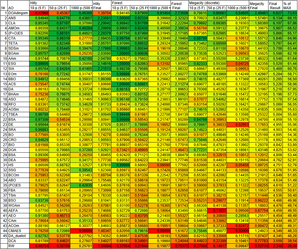
Figure 3. Color-coded ranking of algorithms based on the corresponding tests

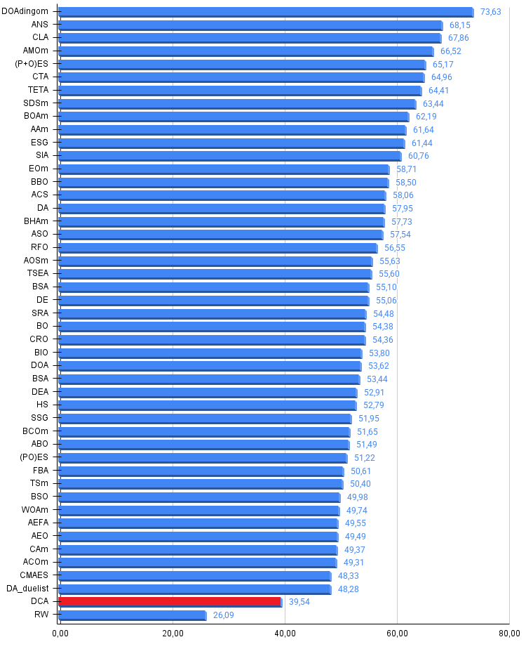
Figure 4. A histogram of the algorithm testing results (on a scale from 0 to 100; the higher the score, the better, where 100 is the maximum possible theoretical result; the archive contains a script for calculating the ranking table)

Pros and cons of the DCA algorithm:

Pros:

1. Fast.
2. Best results on medium- and high-dimensional functions.

Cons:

1. Weaker results on low-dimensional functions.

An archive containing the latest versions of the algorithm source code is attached to this article. The author of this article does not vouch for the absolute accuracy of the descriptions of the canonical algorithms; many of them have been modified to improve their search capabilities. The conclusions and judgments presented in the articles are based on the results of the experiments conducted.

• GitHub: https://github.com/JQSakaJoo/Population-optimization-algorithms-MQL5

Programs used in the article

#	Name	Type	Description
1	#C_AO.mqh	Include file	Parent class for population-based optimization algorithms
2	#C_AO_enum.mqh	Include file	Enumeration of population-based optimization algorithms
3	TestFunctions.mqh	Include file	Benchmark function library
4	TestStandFunctions.mqh	Include file	Library of test bench functions
5	Utilities.mqh	Include file	Library of utility functions
6	CalculationTestResults.mqh	Include file	Script for calculating results for a comparison table
7	Testing AOs.mq5	Script	A unified test bench for all population-based optimization algorithms
8	Simple use of population optimization algorithms.mq5	Script	A simple example of using population-based optimization algorithms without visualization
9	Test_AO_DCA.mq5	Script	Test bench for DCA