

Elite Crystal Evolution Algorithm (CEO-inspired): Practical Implementation
 1 175
1 175
 0
0

Contents
Implementation of the Algorithm
We continue our discussion of the specific methods of the ECEA optimization algorithm, the concept of which was introduced in the previous article. Let me remind you that the developed algorithm operates on a population of crystals that are dynamically divided into two groups: elite (analogous to frozen crystals) and regular (analogous to unfrozen crystals). Elite crystals perform an intensive local search with an adaptively decreasing step size, ensuring exploitation of the identified promising regions. Regular crystals use three movement strategies with probabilities of 40–30–30 percent: directed movement toward the globally best solution (exploitation), movement toward the nearest elite agent and the center of mass of the elite group (moderate exploitation), and exploratory random jumps at two scales (exploration). A periodic "wind" effect regenerates the worst non-elite crystals with a probability of ten percent, ensuring population diversification. All right, let's keep going.
The MoveTowardsEliteCluster function is designed to move a non-elite agent (crystal) toward the group of best (elite) agents.
Finding the nearest elite agent:first, the FindNearestElite(idx) function is called to find the index of the elite agent closest to the current agent (with index idx). If there are no elite agents (nearestElite < 0), the function terminates, since there is nothing to move toward.
Movement along each dimension (coordinate):the method then iterates through all dimensions (coordinates "c") of the current agent. Two direction vectors are calculated:
- toElite — the difference between the coordinate of the nearest elite agent and the agent's current coordinate; it points toward the nearest elite agent.
- toCenter — the difference between the coordinate of the "center of mass" of all elite agents and the agent's current coordinate; it points to the averaged position of the elite agents.
Two random numbers, "r1" and "r2," are generated between 0.0 and 1.0. These numbers are used to weight the influence of each of the two directions (toward the nearest elite agent and toward the center of mass of the elite agents). The agent's current coordinate is updated by adding the following:
- r1 * 0.3 * toElite — the portion of the movement directed toward the nearest elite agent. A fixed coefficient of 0.3 determines how strongly the agent will be drawn toward the nearest elite agent.
- r2 * 0.2 * toCenter — the component of motion directed toward the center of mass of the elite agents. A fixed coefficient of 0.2 determines how strongly the agent will tend toward the average position of the elite agents.
After summing these components, the new coordinate value is passed through the "u.SeInDiSp" function. As before, this function ensures that the coordinate value remains within the allowed bounds and conforms to the specified step size.
This method helps non-elite agents move closer to areas where good solutions have already been found. The agent does not simply move in one direction; instead, it combines movement toward the nearest strong solution with movement toward the common "center of attraction" of all strong solutions. The random weighting coefficients "r1"and "r2"add an element of stochasticity to help avoid getting stuck in the same place.
//————————————————————————————————————————————————————————————————————
void C_AO_ECEA::MoveTowardsEliteCluster (int idx)
{
  int nearestElite = FindNearestElite (idx);
  if (nearestElite < 0) return;

  for (int c = 0; c < coords; c++)
  {
    // Movement toward the nearest elite agent
    double toElite = a [nearestElite].c [c] - a [idx].c [c];
    // Movement toward the center of mass of elite agents
    double toCenter = centerMass [c] - a [idx].c [c];

    double r1 = u.RNDfromCI (0.0, 1.0);
    double r2 = u.RNDfromCI (0.0, 1.0);

    a [idx].c [c] = a [idx].c [c] + r1 * 0.3 * toElite + r2 * 0.2 * toCenter;
    a [idx].c [c] = u.SeInDiSp (a [idx].c [c], rangeMin [c], rangeMax [c], rangeStep [c]);
  }
}
//————————————————————————————————————————————————————————————————————
The ExploratoryMove procedure is designed to move an agent randomly in order to explore the solution space.
The agent with index "idx" will make a random move. The method iterates over all dimensions (coordinates "c") of the current agent, and for each coordinate, it calculates "range" — the full range of valid values for that coordinate, from the minimum (rangeMin[c]) to the maximum (rangeMax[c]). A random number "r" is generated in the range from 0.0 to 1.0. This number determines what type of exploration will be conducted:
- If "r" is less than 0.7 (70% of the time), the agent takes a small step that promotes local exploration of a particular region of the solution space. The magnitude of this step is determined as a random value from -1.0 to 1.0, multiplied by the full "range", by the "explorationRate" coefficient (which controls the overall exploration intensity), and by 0.1 (to keep the step relatively small).
- Otherwise (30% of the time), the agent takes a large leap, which facilitates global exploration of large regions of the solution space. The size of this step is determined in the same way, but is multiplied by 0.5 (which makes the jump significantly larger than during local exploration).
The current value of the agent's coordinate (a [idx].c [c]) is updated by adding the calculated "move", and is then passed through the u.SeInDiSp function.
This method introduces an element of randomness into the agent's behavior, allowing it to leave areas that have already been explored and find new, potentially better solutions. The procedure ensures balanced exploration: in most cases, the agent takes small steps to fine-tune solutions close to the current ones, but periodically takes large leaps to cover broader regions of the search space. The explorationRate coefficient allows controlling the overall activity of exploration moves.
//————————————————————————————————————————————————————————————————————
void C_AO_ECEA::ExploratoryMove (int idx)
{
  for (int c = 0; c < coords; c++)
  {
    double range = rangeMax [c] - rangeMin [c];

    // A simple yet effective method for exploration
    double r = u.RNDfromCI (0.0, 1.0);

    double move;
    if (r < 0.7)
    {
      // 70%: small steps (local exploration)
      move = u.RNDfromCI (-1.0, 1.0) * range * explorationRate * 0.1;
    }
    else
    {
      // 30%: large leaps (global exploration)
      move = u.RNDfromCI (-1.0, 1.0) * range * explorationRate * 0.5;
    }

    a [idx].c [c] = a [idx].c [c] + move;
    a [idx].c [c] = u.SeInDiSp (a [idx].c [c], rangeMin [c], rangeMax [c], rangeStep [c]);
  }
}
//————————————————————————————————————————————————————————————————————
The following method describes the "wind" effect, which is a mechanism for moving the worst non-elite agent (crystal) in order to update its position and potentially find a better solution.
Search for the worst non-elite agent:the variable worstNonElite is initialized to -1 (the worst agent has not yet been found), and worstFitness is initialized to the maximum possible value (DBL_MAX). The function iterates over all agents in the population of popSize. For each agent, the function checks whether it is non-elite and whether its fitness (a [i].f) is worse than the current worstFitness value. If both conditions are met, then that agent becomes the new "worst" (the worstFitness and worstNonElite values are updated).
Checking for the worst agent:if worstNonElite remains -1, this means that either there are no non-elite agents, or they all have equally "good" (or "bad," depending on the interpretation) fitness, making it impossible to identify the worst one. In this case, the function terminates.
Movement of the worst agent:a random "strategy" number is generated in the range from 0.0 to 1.0, which determines exactly how the worst agent will move.
If strategy is less than 0.5 (50% of the time),the agent moves near the best solution. For each coordinate "c":
- the range for the given coordinate is calculated,
- a small amount of random "noise" is generated within ±30% of the full range,
- the agent's new position is set to (cB [c] + noise),
- the coordinate value is forcibly restricted to the allowable minimum (rangeMin [c]) and maximum (rangeMax [c]) values,
- The final adjustment of the coordinate value is performed using u.SeInDiSp to ensure that it matches the rangeStep [c] step size and the boundaries.
Otherwise (in 50% of cases),the agent moves to a completely random location within the allowable boundaries. For each coordinate "c":
- a random number "xi" between 0.0 and 1.0 is generated,
- the new position is set as: rangeMin [c] + xi * (rangeMax [c] - rangeMin [c]) — this ensures that the value is uniformly distributed between the minimum and the maximum,
- the final correction of the coordinate value is performed using u.SeInDiSp.
The "wind" mechanism aims to "shake up" the system by removing the least successful non-elite agents and placing them in new, potentially more promising positions. This helps prevent stagnation, where the population consists mainly of similar, relatively ineffective solutions. A move can be either local, near the best solution found so far, or completely random, giving the algorithm a chance to discover an entirely new region of the search space.
//————————————————————————————————————————————————————————————————————
void C_AO_ECEA::WindEffect ()
{
  // The "wind" destroys the worst non-elite agents and moves them
  int worstNonElite = -1;
  double worstFitness = DBL_MAX;

  for (int i = 0; i < popSize; i++)
  {
    if (!crystalData [i].isElite && a [i].f < worstFitness)
    {
      worstFitness  = a [i].f;
      worstNonElite = i;
    }
  }

  if (worstNonElite < 0) return;

  // Move to a new location
  double strategy = u.RNDfromCI (0.0, 1.0);

  if (strategy < 0.5)
  {
    // Near the best solution
    for (int c = 0; c < coords; c++)
    {
      double range = rangeMax [c] - rangeMin [c];
      double noise = u.RNDfromCI (-1.0, 1.0) * range * 0.3;
      a [worstNonElite].c [c] = cB [c] + noise;

      if (a [worstNonElite].c [c] < rangeMin [c]) a [worstNonElite].c [c] = rangeMin [c];
      if (a [worstNonElite].c [c] > rangeMax [c]) a [worstNonElite].c [c] = rangeMax [c];
      a [worstNonElite].c [c] = u.SeInDiSp (a [worstNonElite].c [c], rangeMin [c], rangeMax [c], rangeStep [c]);
    }
  }
  else
  {
    // Completely randomly
    for (int c = 0; c < coords; c++)
    {
      double xi = u.RNDfromCI (0.0, 1.0);
      a [worstNonElite].c [c] = rangeMin [c] + xi * (rangeMax [c] - rangeMin [c]);
      a [worstNonElite].c [c] = u.SeInDiSp (a [worstNonElite].c [c], rangeMin [c], rangeMax [c], rangeStep [c]);
    }
  }
}
//————————————————————————————————————————————————————————————————————
The FindNearestElite function finds the index of the "elite" agent (crystal) closest to the specified agent. The agent index "idx" specifies the agent for which we are searching for the nearest elite neighbor. The following variables are initialized:
- nearest — set to -1 (which means that the nearest elite agent has not yet been found);
- minDist — initialized to the maximum possible value (DBL_MAX), so that any distance found will be smaller.
- Ignoring the agent itself: if "i" equals "idx" (that is, if this is the same agent for which we are searching for a neighbor), then this agent is skipped (continue).
- Elite check: if agent "i" is not an elite agent, it is skipped. We search only among elite agents.
If agent "i" is an elite agent and is not "idx", the Euclidean distance between agent "idx" and agent "i" is calculated. For each coordinate "c", the difference (diff) between the corresponding coordinates of the agents is calculated. The square of this difference (diff * diff) is added to the total sum of squared differences, "dist". After iterating through all coordinates, the square root operation is applied to "dist" to obtain the actual Euclidean distance.
If the calculated distance "dist" is less than the current minimum distance "minDist", then we have found a new nearest elite agent. "minDist" (the current minimum distance) and "nearest" (the index of this new nearest elite agent) are updated. After iterating through all agents, the function returns the index (nearest) of the nearest elite agent. If no elite agents are found in the population, the function returns -1.
This function is auxiliary and is used to determine which "elite" solution (the most successful agent) another agent should approach.
//————————————————————————————————————————————————————————————————————
int C_AO_ECEA::FindNearestElite (int idx)
{
  int nearest = -1;
  double minDist = DBL_MAX;

  for (int i = 0; i < popSize; i++)
  {
    if (i == idx) continue;
    if (!crystalData [i].isElite) continue;

    double dist = 0.0;
    for (int c = 0; c < coords; c++)
    {
      double diff = a [idx].c [c] - a [i].c [c];
      dist += diff * diff;
    }
    dist = MathSqrt (dist);

    if (dist < minDist)
    {
      minDist = dist;
      nearest = i;
    }
  }

  return nearest;
}
//————————————————————————————————————————————————————————————————————
The CalculateEliteRadii function calculates the radius of influence for each "elite" agent (crystal) based on the distances to other elite agents. The function iterates through all agents in the population; only those agents marked as elite are processed.
Search for the nearest other elite agent. For each elite agent "i", the variable minDistToOtherElite is initialized to the maximum possible value (DBL_MAX) in order to find the minimum distance. A nested loop begins, which again iterates through all agents "j" in the population. We check that we are not comparing an agent with itself (i == j) and that the other agent "j" is also an elite agent (crystalData[j].isElite). The Euclidean distance between elite agent "i" and another elite agent "j" is calculated across all coordinates. If the calculated distance "dist" is less than the current minimum distance minDistToOtherElite, then minDistToOtherElite is updated.
Radius calculation and storage. After the inner loop (in which the minimum distance to another elite agent was found), the radius for the current elite agent "i" is calculated as half of that minimum distance (minDistToOtherElite/2.0). This calculated radius is stored in the data structure associated with agent "i" (crystalData[i].radius).
This mechanism is designed to determine the "region of influence" of each elite solution. The radius is chosen so that it is less than half the distance to the nearest neighbor. This means that the regions of influence of different elite agents should not overlap. This can be useful for maintaining diversity in the population, ensuring that different elite solutions truly represent separate, distinct search regions.
//————————————————————————————————————————————————————————————————————
void C_AO_ECEA::CalculateEliteRadii ()
{
  // Calculate the radii of influence of elite agents based on the distances between them
  for (int i = 0; i < popSize; i++)
  {
    if (!crystalData [i].isElite) continue;

    double minDistToOtherElite = DBL_MAX;

    for (int j = 0; j < popSize; j++)
    {
      if (i == j) continue;
      if (!crystalData [j].isElite) continue;

      double dist = 0.0;
      for (int c = 0; c < coords; c++)
      {
        double diff = a [i].c [c] - a [j].c [c];
        dist += diff * diff;
      }
      dist = MathSqrt (dist);

      if (dist < minDistToOtherElite)
      {
        minDistToOtherElite = dist;
      }
    }

    crystalData [i].radius = minDistToOtherElite / 2.0;
  }
}
//————————————————————————————————————————————————————————————————————
The GetDynamicExplorationRate function dynamically adjusts the exploration rate based on the algorithm's current progress. The main purpose of this function is to reduce the exploration intensity ("exploration rate") as the algorithm runs. In the early stages of the algorithm, it is important to explore new areas, and as it gets closer to an optimal solution, the focus shifts to more precise fine-tuning of the solutions already found.
The "progress" variable (execution progress) is calculated. It is defined as the ratio of the current number of iterations (iterationCount) to a fixed maximum value (100.0). If "progress" exceeds 1.0 (that is, more than 100 iterations have been completed), it is clipped to 1.0 to ensure that the maximum reduction factor is 0.7. The return value is the result of multiplying the base exploration rate (explorationRate) by the reduction factor (1.0 - 0.7 * progress).
In the early stages, "progress" is close to 0. As "progress" increases (as "progress" approaches 1.0), the coefficient will decrease. For example, when "progress" is equal to 1.0, the coefficient will be 1.0 - 0.7 * 1.0 = 0.3. This means that the exploration rate will be reduced to 30% of its base value.
Imagine that you have a "knob" for adjusting exploration. This knob is set to its maximum value at the beginning of the algorithm. The GetDynamicExplorationRate function gradually turns this knob, reducing the exploration intensity. Thus, in the later stages, the algorithm "wanders" less and focuses more on improving the solutions it has found.
//————————————————————————————————————————————————————————————————————
double C_AO_ECEA::GetDynamicExplorationRate ()
{
  // Adaptive exploration intensity
  // Start high and gradually reduce it over time
  double progress = (double)iterationCount / 100.0;
  if (progress > 1.0) progress = 1.0;

  return explorationRate * (1.0 - 0.7 * progress);
}
//————————————————————————————————————————————————————————————————————
The Revision method updates information about the best solution found and tracks stagnation (lack of improvement). Before a possible update, the current best function value (denoted by fB) is stored in the variable prevBest. This is necessary for subsequent comparison. Another function (UpdateEliteStatus) is called, which reviews and, if necessary, changes the "elite" status of agents in the population.
Updating the best solution. The use of [0] implies that agents are sorted or processed in such a way that a [0] always contains the current best solution. The function value for the best agent (a [0].f) is assigned to fB. The coordinates of this best solution, a [0].c, are copied to cB (the variable used to store the coordinates of the best-known solution).
Monitoring stagnation. The current best function value (fB) is compared with the previously saved best value (prevBest). If the difference between them is very small (less than 1e-10, indicating no significant improvement), the stagnation counter (noImprovementCount) is incremented by one. If, however, an improvement has occurred (the difference is greater than 1e-10), the stagnation counter is reset to zero.
This function performs a periodic "revision" of the algorithm's state:
- determines which agents remain "elite";
- records the best solution found so far;
- checks whether the algorithm continues to find new, better solutions, or whether it has "stalled" (stagnation).
//————————————————————————————————————————————————————————————————————
void C_AO_ECEA::Revision ()
{
  double prevBest = fB;

  // Update the status of elite crystals
  UpdateEliteStatus ();
  fB = a [0].f;
  ArrayCopy (cB, a [0].c, 0, 0, coords);

  // Track stagnation
  if (MathAbs (fB - prevBest) < 1e-10) noImprovementCount++;
  else                                 noImprovementCount = 0;
}
//————————————————————————————————————————————————————————————————————
Test Results
The ECEA algorithm was tested on a standard benchmark comprising three types of functions (Hilly, Forest, Megacity) with different problem dimensions (five, twenty-five, and five hundred dimensions), with a budget of 10,000 objective function evaluations per run. Each test was repeated ten times to ensure statistical reliability. The overall ECEA result was 36 percent, which exceeds the baseline random search (26 percent) but falls short of the 45 percent threshold typical of top-performing optimization algorithms.ECEA|Elite Crystal Evolution Algorithm|50.0|10.0|0.5|0.1|
=============================
5 Hilly's; Func runs: 10000; result: 0.6824547309245615
25 Hilly's; Func runs: 10000; result: 0.4467067359108001
500 Hilly's; Func runs: 10000; result: 0.29066242412735266
=============================
5 Forest's; Func runs: 10000; result: 0.6110808506476546
25 Forest's; Func runs: 10000; result: 0.36838637212724284
500 Forest's; Func runs: 10000; result: 0.20596535563655824
=============================
5 Megacity's; Func runs: 10000; result: 0.36
25 Megacity's; Func runs: 10000; result: 0.2033846153846154
500 Megacity's; Func runs: 10000; result: 0.11233846153846264
=============================
All score: 3.28098 (36.46%)
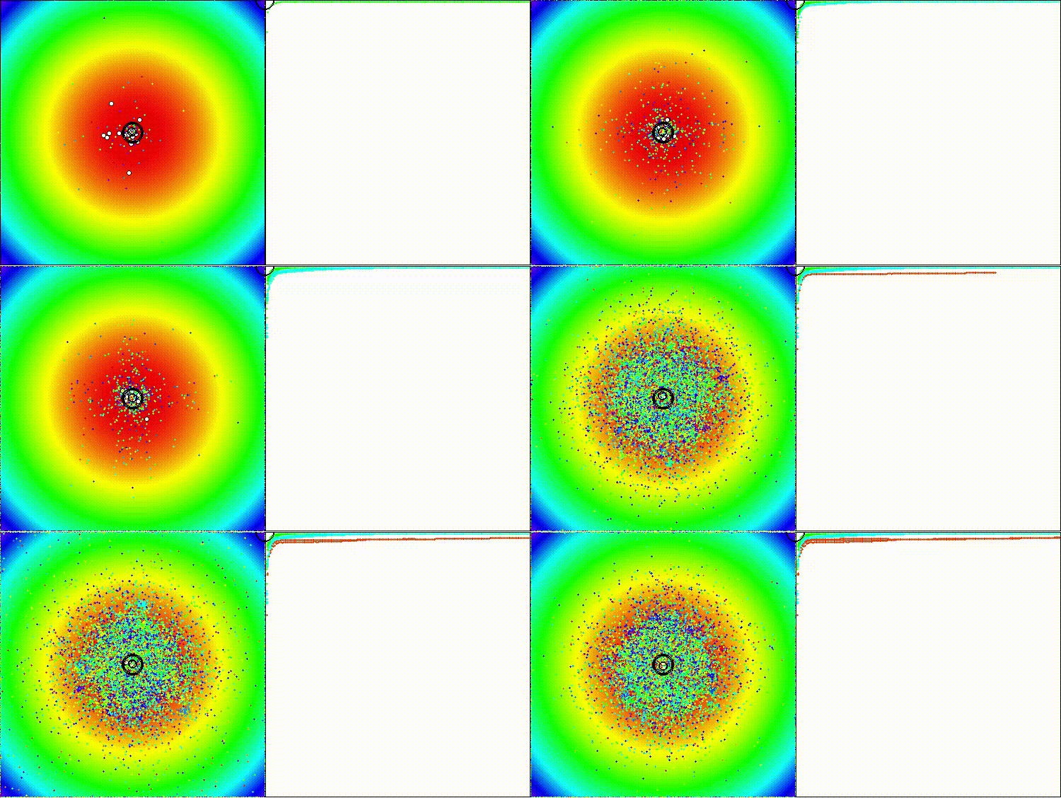
Crystallization structures are visible in the visualization; the algorithm's search capabilities are more pronounced on medium-dimensional functions.
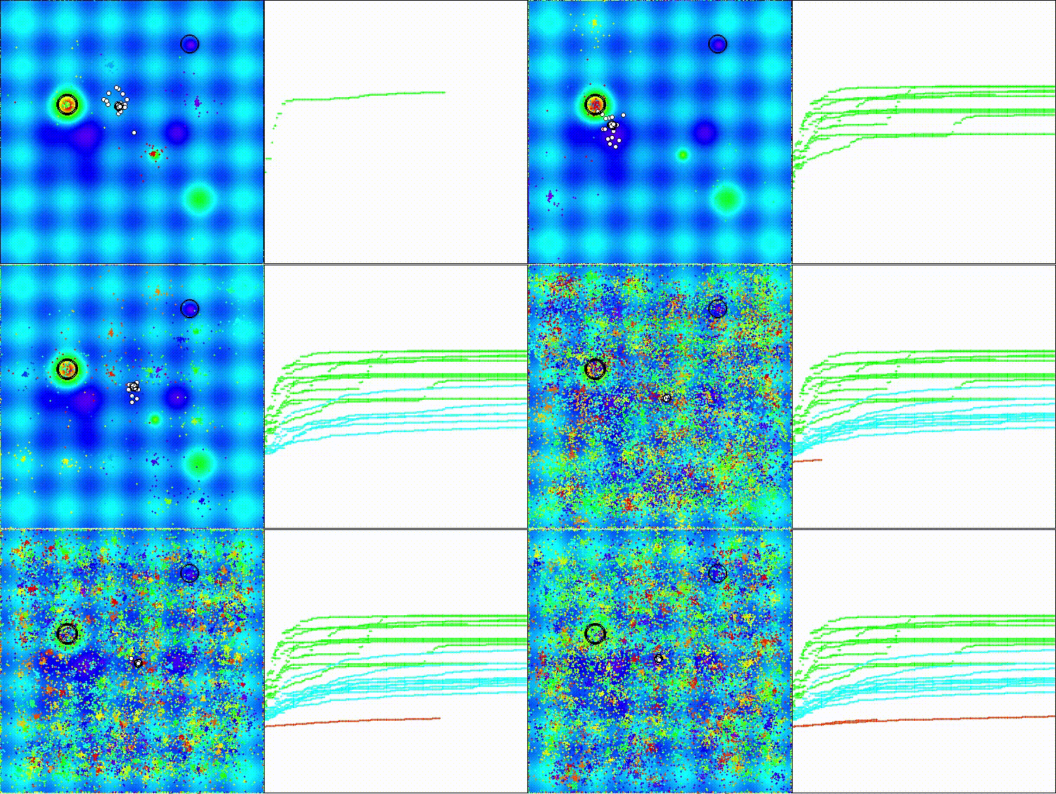
ECEA on the Hilly test function
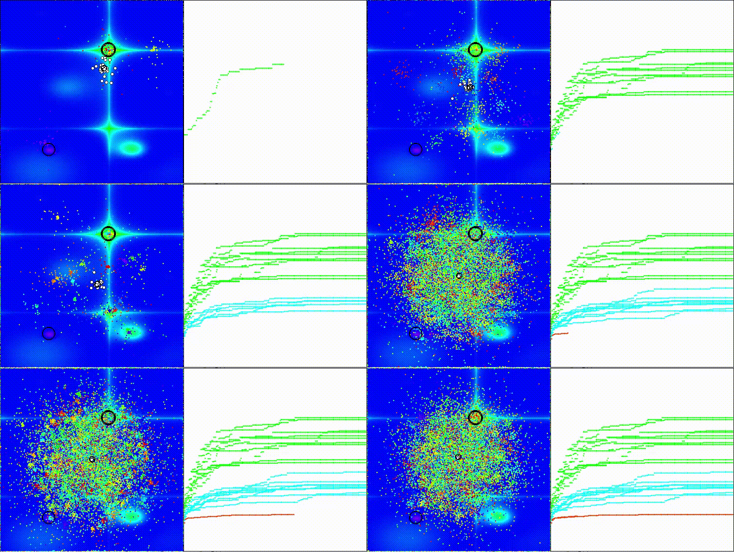
ECEA on the Forest test function
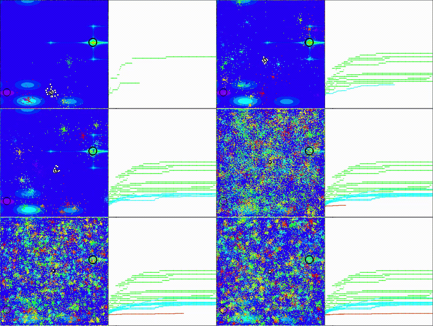
ECEA on the Megacity test function
Let's also take a look at how the ECEA algorithm performs on standard functions that are not included in our ranking of population-based algorithms but are commonly used for testing. As you can see, the algorithm shows very high convergence on these types of problems; therefore, each algorithm should be tested on various types of functions to determine the conditions under which its full potential is best realized.
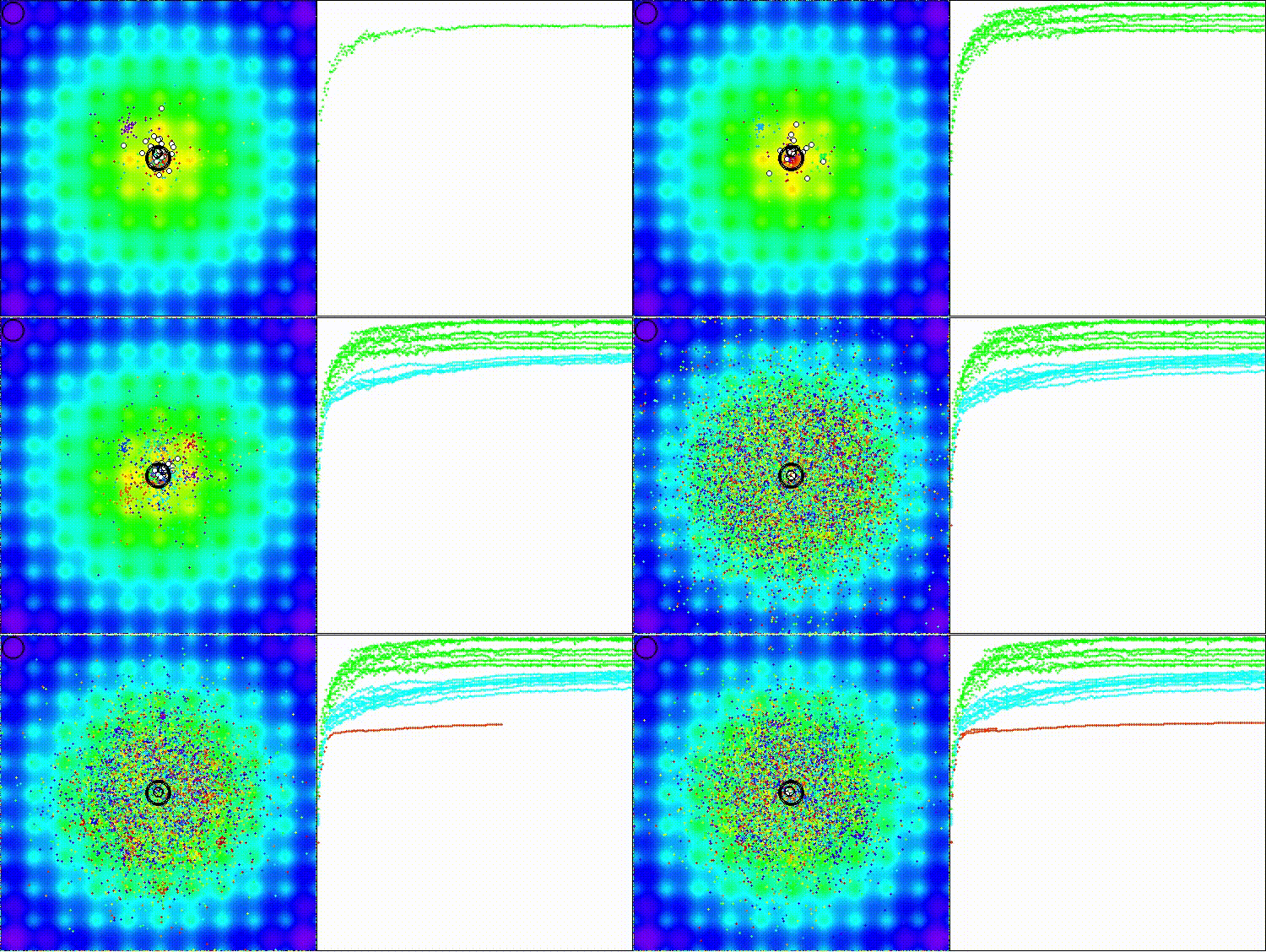
ECEA on the standard Ackley test function
ECEA on the standard Paraboloid test function
The ECEA algorithm is included in the ranking table for reference.
| No. | AO | Description | Hilly | Hilly Final | Forest | Forest Final | Megacity (discrete) | Megacity Final | Final Result | % of MAX | ||||||
| 10 p (5 F) | 50 p (25 F) | 1000 p (500 F) | 10 p (5 F) | 50 p (25 F) | 1000 p (500 F) | 10 p (5 F) | 50 p (25 F) | 1,000 p (500 F) | ||||||||
| 1 | DOAdingom | dingo_optimization_algorithm_M | 0.47968 | 0.45367 | 0.46369 | 1.39704 | 0.94145 | 0.87909 | 0.91454 | 2.73508 | 0.78615 | 0.86061 | 0.84805 | 2.49481 | 6.627 | 73.63 |
| 2 | ANS | across neighbourhood search | 0.94948 | 0.84776 | 0.43857 | 2.23581 | 1.00000 | 0.92334 | 0.39988 | 2.32323 | 0.70923 | 0.63477 | 0.23091 | 1.57491 | 6.134 | 68.15 |
| 3 | CLA | code lock algorithm (joo) | 0.95345 | 0.87107 | 0.37590 | 2.20042 | 0.98942 | 0.91709 | 0.31642 | 2.22294 | 0.79692 | 0.69385 | 0.19303 | 1.68380 | 6.107 | 67.86 |
| 4 | AMOm | animal migration optimization M | 0.90358 | 0.84317 | 0.46284 | 2.20959 | 0.99001 | 0.92436 | 0.46598 | 2.38034 | 0.56769 | 0.59132 | 0.23773 | 1.39675 | 5.987 | 66.52 |
| 5 | (P+O)ES | (P+O) evolution strategies | 0.92256 | 0.88101 | 0.40021 | 2.20379 | 0.97750 | 0.87490 | 0.31945 | 2.17185 | 0.67385 | 0.62985 | 0.18634 | 1.49003 | 5.866 | 65.17 |
| 6 | CTA | comet tail algorithm (joo) | 0.95346 | 0.86319 | 0.27770 | 2.09435 | 0.99794 | 0.85740 | 0.33949 | 2.19484 | 0.88769 | 0.56431 | 0.10512 | 1.55712 | 5.846 | 64.96 |
| 7 | TETA | time evolution travel algorithm (joo) | 0.91362 | 0.82349 | 0.31990 | 2.05701 | 0.97096 | 0.89532 | 0.29324 | 2.15952 | 0.73462 | 0.68569 | 0.16021 | 1.58052 | 5.797 | 64.41 |
| 8 | SDSm | stochastic diffusion search M | 0.93066 | 0.85445 | 0.39476 | 2.17988 | 0.99983 | 0.89244 | 0.19619 | 2.08846 | 0.72333 | 0.61100 | 0.10670 | 1.44103 | 5.709 | 63.44 |
| 9 | BOAm | billiards optimization algorithm M | 0.95757 | 0.82599 | 0.25235 | 2.03590 | 1.00000 | 0.90036 | 0.30502 | 2.20538 | 0.73538 | 0.52523 | 0.09563 | 1.35625 | 5.598 | 62.19 |
| 10 | AAm | archery algorithm M | 0.91744 | 0.70876 | 0.42160 | 2.04780 | 0.92527 | 0.75802 | 0.35328 | 2.03657 | 0.67385 | 0.55200 | 0.23738 | 1.46323 | 5.548 | 61.64 |
| 11 | ESG | evolution of social groups (joo) | 0.99906 | 0.79654 | 0.35056 | 2.14616 | 1.00000 | 0.82863 | 0.13102 | 1.95965 | 0.82333 | 0.55300 | 0.04725 | 1.42358 | 5.529 | 61.44 |
| 12 | SIA | simulated isotropic annealing (joo) | 0.95784 | 0.84264 | 0.41465 | 2.21513 | 0.98239 | 0.79586 | 0.20507 | 1.98332 | 0.68667 | 0.49300 | 0.09053 | 1.27020 | 5.469 | 60.76 |
| 13 | EOm | extremal_optimization_M | 0.76166 | 0.77242 | 0.31747 | 1.85155 | 0.99999 | 0.76751 | 0.23527 | 2.00277 | 0.74769 | 0.53969 | 0.14249 | 1.42987 | 5.284 | 58.71 |
| 14 | BBO | biogeography-based optimization | 0.94912 | 0.69456 | 0.35031 | 1.99399 | 0.93820 | 0.67365 | 0.25682 | 1.86867 | 0.74615 | 0.48277 | 0.17369 | 1.40261 | 5.265 | 58.50 |
| 15 | ACS | artificial cooperative search | 0.75547 | 0.74744 | 0.30407 | 1.80698 | 1.00000 | 0.88861 | 0.22413 | 2.11274 | 0.69077 | 0.48185 | 0.13322 | 1.30583 | 5.226 | 58.06 |
| 16 | DA | dialectical algorithm | 0.86183 | 0.70033 | 0.33724 | 1.89940 | 0.98163 | 0.72772 | 0.28718 | 1.99653 | 0.70308 | 0.45292 | 0.16367 | 1.31967 | 5.216 | 57.95 |
| 17 | BHAm | black hole algorithm M | 0.75236 | 0.76675 | 0.34583 | 1.86493 | 0.93593 | 0.80152 | 0.27177 | 2.00923 | 0.65077 | 0.51646 | 0.15472 | 1.32195 | 5.196 | 57.73 |
| 18 | ASO | anarchy society optimization | 0.84872 | 0.74646 | 0.31465 | 1.90983 | 0.96148 | 0.79150 | 0.23803 | 1.99101 | 0.57077 | 0.54062 | 0.16614 | 1.27752 | 5.178 | 57.54 |
| 19 | RFO | royal flush optimization (joo) | 0.83361 | 0.73742 | 0.34629 | 1.91733 | 0.89424 | 0.73824 | 0.24098 | 1.87346 | 0.63154 | 0.50292 | 0.16421 | 1.29867 | 5.089 | 56.55 |
| 20 | AOSm | atomic orbital search M | 0.80232 | 0.70449 | 0.31021 | 1.81702 | 0.85660 | 0.69451 | 0.21996 | 1.77107 | 0.74615 | 0.52862 | 0.14358 | 1.41835 | 5.006 | 55.63 |
| 21 | TSEA | turtle shell evolution algorithm (joo) | 0.96798 | 0.64480 | 0.29672 | 1.90949 | 0.99449 | 0.61981 | 0.22708 | 1.84139 | 0.69077 | 0.42646 | 0.13598 | 1.25322 | 5.004 | 55.60 |
| 22 | BSA | backtracking_search_algorithm | 0.97309 | 0.54534 | 0.29098 | 1.80941 | 0.99999 | 0.58543 | 0.21747 | 1.80289 | 0.84769 | 0.36953 | 0.12978 | 1.34700 | 4.959 | 55.10 |
| 23 | DE | differential evolution | 0.95044 | 0.61674 | 0.30308 | 1.87026 | 0.95317 | 0.78896 | 0.16652 | 1.90865 | 0.78667 | 0.36033 | 0.02953 | 1.17653 | 4.955 | 55.06 |
| 24 | SRA | successful restaurateur algorithm (joo) | 0.96883 | 0.63455 | 0.29217 | 1.89555 | 0.94637 | 0.55506 | 0.19124 | 1.69267 | 0.74923 | 0.44031 | 0.12526 | 1.31480 | 4.903 | 54.48 |
| 25 | CRO | chemical reaction optimization | 0.94629 | 0.66112 | 0.29853 | 1.90593 | 0.87906 | 0.58422 | 0.21146 | 1.67473 | 0.75846 | 0.42646 | 0.12686 | 1.31178 | 4.892 | 54.36 |
| 26 | BIO | blood inheritance optimization (joo) | 0.81568 | 0.65336 | 0.30877 | 1.77781 | 0.89937 | 0.65319 | 0.21760 | 1.77016 | 0.67846 | 0.47631 | 0.13902 | 1.29378 | 4.842 | 53.80 |
| 27 | DOA | dream_optimization_algorithm | 0.85556 | 0.70085 | 0.37280 | 1.92921 | 0.73421 | 0.48905 | 0.24147 | 1.46473 | 0.77231 | 0.47354 | 0.18561 | 1.43146 | 4.825 | 53.62 |
| 28 | BSA | bird swarm algorithm | 0.89306 | 0.64900 | 0.26250 | 1.80455 | 0.92420 | 0.71121 | 0.24939 | 1.88479 | 0.69385 | 0.32615 | 0.10012 | 1.12012 | 4.809 | 53.44 |
| 29 | DEA | dolphin_echolocation_algorithm | 0.75995 | 0.67572 | 0.34171 | 1.77738 | 0.89582 | 0.64223 | 0.23941 | 1.77746 | 0.61538 | 0.44031 | 0.15115 | 1.20684 | 4.762 | 52.91 |
| 30 | HS | harmony search | 0.86509 | 0.68782 | 0.32527 | 1.87818 | 0.99999 | 0.68002 | 0.09590 | 1.77592 | 0.62000 | 0.42267 | 0.05458 | 1.09725 | 4.751 | 52.79 |
| 31 | SSG | saplings sowing and growing | 0.77839 | 0.64925 | 0.39543 | 1.82308 | 0.85973 | 0.62467 | 0.17429 | 1.65869 | 0.64667 | 0.44133 | 0.10598 | 1.19398 | 4.676 | 51.95 |
| 32 | BCOm | bacterial chemotaxis optimization M | 0.75953 | 0.62268 | 0.31483 | 1.69704 | 0.89378 | 0.61339 | 0.22542 | 1.73259 | 0.65385 | 0.42092 | 0.14435 | 1.21912 | 4.649 | 51.65 |
| 33 | ABO | african buffalo optimization | 0.83337 | 0.62247 | 0.29964 | 1.75548 | 0.92170 | 0.58618 | 0.19723 | 1.70511 | 0.61000 | 0.43154 | 0.13225 | 1.17378 | 4.634 | 51.49 |
| 34 | (PO)ES | (PO) evolution strategies | 0.79025 | 0.62647 | 0.42935 | 1.84606 | 0.87616 | 0.60943 | 0.19591 | 1.68151 | 0.59000 | 0.37933 | 0.11322 | 1.08255 | 4.610 | 51.22 |
| 35 | FBA | fractal-based algorithm | 0.79000 | 0.65134 | 0.28965 | 1.73099 | 0.87158 | 0.56823 | 0.18877 | 1.62858 | 0.61077 | 0.46062 | 0.12398 | 1.19537 | 4.555 | 50.61 |
| 36 | TSm | tabu search M | 0.87795 | 0.61431 | 0.29104 | 1.78330 | 0.92885 | 0.51844 | 0.19054 | 1.63783 | 0.61077 | 0.38215 | 0.12157 | 1.11449 | 4.536 | 50.40 |
| 37 | BSO | brain storm optimization | 0.93736 | 0.57616 | 0.29688 | 1.81041 | 0.93131 | 0.55866 | 0.23537 | 1.72534 | 0.55231 | 0.29077 | 0.11914 | 0.96222 | 4.498 | 49.98 |
| 38 | WOAm | whale optimization algorithm M | 0.84521 | 0.56298 | 0.26263 | 1.67081 | 0.93100 | 0.52278 | 0.16365 | 1.61743 | 0.66308 | 0.41138 | 0.11357 | 1.18803 | 4.476 | 49.74 |
| 39 | AEFA | artificial electric field algorithm | 0.87700 | 0.61753 | 0.25235 | 1.74688 | 0.92729 | 0.72698 | 0.18064 | 1.83490 | 0.66615 | 0.11631 | 0.09508 | 0.87754 | 4.459 | 49.55 |
| 40 | AEO | artificial ecosystem-based optimization algorithm | 0.91380 | 0.46713 | 0.26470 | 1.64563 | 0.90223 | 0.43705 | 0.21400 | 1.55327 | 0.66154 | 0.30800 | 0.28563 | 1.25517 | 4.454 | 49.49 |
| 41 | CAm | camel algorithm M | 0.78684 | 0.56042 | 0.35133 | 1.69859 | 0.82772 | 0.56041 | 0.24336 | 1.63149 | 0.64846 | 0.33092 | 0.13418 | 1.11356 | 4.444 | 49.37 |
| 42 | ACOm | ant colony optimization M | 0.88190 | 0.66127 | 0.30377 | 1.84693 | 0.85873 | 0.58680 | 0.15051 | 1.59604 | 0.59667 | 0.37333 | 0.02472 | 0.99472 | 4.438 | 49.31 |
| 43 | CMAES | covariance_matrix_adaptation_evolution_strategy | 0.76258 | 0.72089 | 0.00000 | 1.48347 | 0.82056 | 0.79616 | 0.00000 | 1.61672 | 0.75846 | 0.49077 | 0.00000 | 1.24923 | 4.349 | 48.33 |
| 44 | DA_duelist | duelist_algorithm | 0.92782 | 0.53778 | 0.27792 | 1.74352 | 0.86957 | 0.47536 | 0.18193 | 1.52686 | 0.62153 | 0.33569 | 0.11715 | 1.07437 | 4.345 | 48.28 |
| 45 | BFO-GA | bacterial foraging optimization - GA | 0.89150 | 0.55111 | 0.31529 | 1.75790 | 0.96982 | 0.39612 | 0.06305 | 1.42899 | 0.72667 | 0.27500 | 0.03525 | 1.03692 | 4.224 | 46.93 |
| ECEA | elite crystal evolution algorithm | 0.68245 | 0.44671 | 0.29066 | 1.41982 | 0.61108 | 0.36838 | 0.20597 | 1.18543 | 0.36000 | 0.20338 | 0.11233 | 0.67571 | 3.281 | 36.46 | |
| RW | random walk | 0.48754 | 0.32159 | 0.25781 | 1.06694 | 0.37554 | 0.21944 | 0.15877 | 0.75375 | 0.27969 | 0.14917 | 0.09847 | 0.52734 | 2.348 | 26.09 | |
Conclusions
The ECEA algorithm represents an attempt to adapt the crystallization concept from the original Crystal Energy Optimizer algorithm — developed for combinatorial problems — to the field of continuous optimization in multidimensional real-valued spaces. Experimental evaluation on our benchmark functions showed that the developed algorithm achieves a score of 36%, outperforming random search. This result indicates that the algorithm does indeed work and possesses meaningful search capabilities that surpass those of primitive methods; however, it does not reach the threshold required to be ranked among the best optimization algorithms.
An analysis of the reasons behind these results highlights the difficulty of directly adapting algorithms from the combinatorial domain to the continuous domain. The original CEO is based on specific mechanisms that make sense only for discrete structures, such as the graph of connections between route solutions in the traveling salesman problem, physical heat-transfer formulas in which the influence of the lake center is inversely proportional to distance, interaction between pairs of connected frozen crystals via triangular distances, and the process of depositing new crystals at positions between existing neighbors, with existing bonds being broken and new ones formed. In the process of adapting it into ECEA, all of these unique mechanisms were radically simplified, since they have no direct analogues in the geometry of continuous space. Ultimately, only the high-level conceptual ideas from the original algorithm remained: the division of the population into elite and ordinary agents, the presence of a central attractor, periodic diversification through the wind effect, and the balance between exploration and exploitation.
Despite the limitations, the work on the development of ECEA has certain scientific and practical value. The developed implementation is fully functional, stable, free of obvious implementation errors, and can be used as a baseline version for further exploration and improvement. The simplicity of the algorithm — with just four configurable parameters — makes it easy to understand and modify, which is useful for educational purposes and for quickly prototyping ideas.
There are several avenues for improving the algorithm. Incorporating an opposition-based learning mechanism — where, for each crystal, its opposite point in the search space is also considered — can help avoid situations where the entire population becomes concentrated in the wrong region. Periodic low-probability mutation of elite crystals can prevent them from getting stuck in local optima.
In conclusion, it should be noted that the experiment in adapting CEO for continuous optimization can be considered successful from a scientific research perspective, as it identified and demonstrated the key challenges of such adaptation and showed that the direct transfer of combinatorial algorithms to the continuous domain requires not merely the replacement of operators, but a rethinking of the underlying mechanisms. From a practical standpoint, the result is intermediate: the algorithm operates stably and outperforms random search, but does not match the performance of the best population-based optimization methods.
ECEA can be recommended as a teaching example of how to adapt nature-inspired algorithms, as a starting point for further improvements, or as a simple and straightforward method. The main contribution of this work lies not so much in the development of a highly efficient algorithm as in the systematic investigation of the process of cross-domain adaptation of metaheuristics.
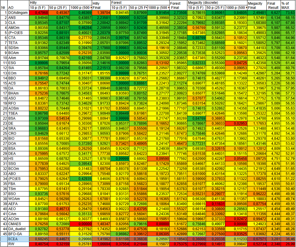
Figure 2. Color coding of algorithms for the corresponding tests
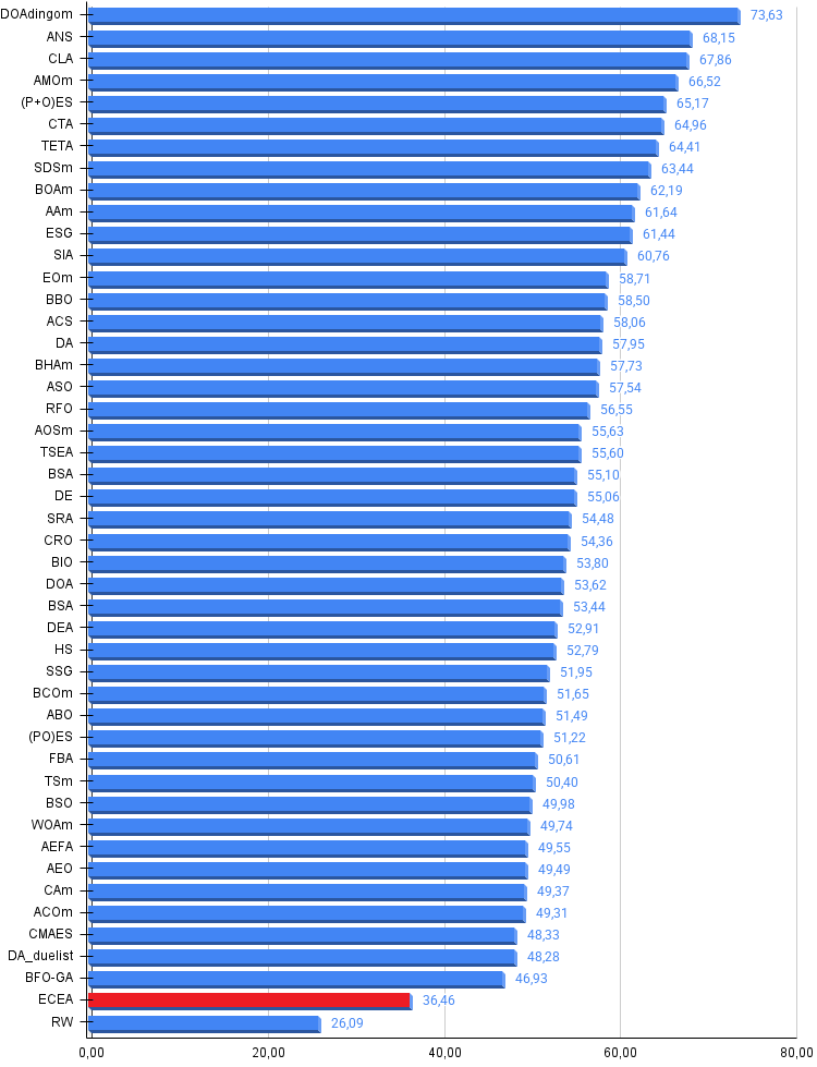
Figure 3. Histogram of algorithm test results (on a scale from 0 to 100; the higher the score, the better, where 100 is the maximum possible theoretical result; the archive contains a script for calculating the ranking table)
Pros and Cons of theECEA Algorithm:
Pros:
- Fast.
- Best results on medium- and high-dimensional functions.
Cons:
- Weaker results on low-dimensional functions.
An archive containing the latest versions of the source code for the algorithms is attached to the article. The author of this article does not guarantee the absolute accuracy of the descriptions of the canonical algorithms; changes have been made to many of them to improve their search capabilities. The conclusions and judgments presented in the articles are based on the results of the experiments conducted.
Programs used in the article
| # | Name | Type | Description |
|---|---|---|---|
| 1 | #C_AO.mqh | Include file | Parent class of population-based optimization algorithms |
| 2 | #C_AO_enum.mqh | Include file | Enumeration of population-based optimization algorithms |
| 3 | TestFunctions.mqh | Include file | Library of test functions |
| 4 | TestStandFunctions.mqh | Include file | Library of test bench functions |
| 5 | Utilities.mqh | Include file | Library of utility functions |
| 6 | CalculationTestResults.mqh | Include file | Script for calculating results for the comparison table |
| 7 | Testing AOs.mq5 | Script | A unified test bench for all population-based optimization algorithms |
| 8 | Simple use of population optimization algorithms.mq5 | Script | A simple example of using population-based optimization algorithms without visualization |
| 9 | Test_AO_ECEA.mq5 | Script | Test bench for ECEA |
Translated from Russian by MetaQuotes Ltd.
Original article: https://www.mql5.com/ru/articles/20240
Warning: All rights to these materials are reserved by MetaQuotes Ltd. Copying or reprinting of these materials in whole or in part is prohibited.
This article was written by a user of the site and reflects their personal views. MetaQuotes Ltd is not responsible for the accuracy of the information presented, nor for any consequences resulting from the use of the solutions, strategies or recommendations described.

 Building Volatility Models in MQL5 (Part V): Implementing EGARCH as an Alternate Asymmetric Volatility Process
 Feature Engineering for ML (Part 12): Fractal Features in MQL5
 A Trailing Stop Engine in MQL5 Supporting Five Trail Methods Simultaneously
 Price Action Analysis Toolkit Development (Part 78): Extending the Indicator Search Panel with Symbol Selection in MQL5

- Free trading apps
- Over 8,000 signals for copying
- Economic news for exploring financial markets
You agree to website policy and terms of use