Differential Search Algorithm (DSA)

Contents

1. Introduction
2. Algorithm Implementation
3. Test Results
4. Conclusions

Introduction

In this article, we will examine the Differential Search Algorithm — an optimization algorithm that mimics the migration of a superorganism (a swarm) in search of better conditions. DSA was proposed by Pinar Civicioglu in 2012 as an alternative to classical algorithms such as PSO (Particle Swarm Optimization) and DE (Differential Evolution). It models the behavior of a population of organisms that move within the solution space, simulating natural migration with elements of randomness and directed search. Here is one of the publications on this algorithm.

Algorithm Implementation

DSA simulates the migration of a superorganism (a flock or swarm) in search of better conditions. Imagine a flock of birds flying from place to place in search of food; this is a population of solutions moving through the search space. At each iteration, each individual chooses a direction — where to move (toward a random individual, toward top individuals, or toward the best individual) — and takes a step; the step size is determined by a Gamma distribution, which produces many small steps and occasional large jumps.

A step can be negative — in which case the individual moves in the opposite direction. During a partial rollback, randomly selected coordinates are restored to their previous values. This preserves good genes and allows individual parameters to be fine-tuned. The algorithm then decides whether to accept the move: if the new position is better than the old one, the individual stays there; otherwise, it returns to the previous position.

1. Superorganism (Population). This is a set of individuals (solutions). Each individual is a point in the search space.

Example: Find the optimum of the function f(x, y). A population of 5 individuals:

Individual 0: (2.5, 3.1) fitness = 0.65
Individual 1: (1.2, 4.0) fitness = 0.42
Individual 2: (3.8, 2.5) fitness = 0.78 ← best
Individual 3: (0.5, 1.0) fitness = 0.31
Individual 4: (2.0, 2.0) fitness = 0.55

2. Migration direction (Direction). Where will each individual move? There are 4 strategies:

B-DSA (Bijective) — Random permutation. Each individual moves toward another randomly selected individual.

Example: Index permutation: [0,1,2,3,4] → [3,0,4,2,1]

Individual 0 → moves toward individual 3: direction = (0.5, 1.0)
Individual 1 → moves toward individual 0: direction = (2.5, 3.1)
Individual 2 → moves toward individual 4: direction = (2.0, 2.0)
Individual 3 → moves toward individual 2: direction = (3.8, 2.5)
Individual 4 → moves toward individual 1: direction = (1.2, 4.0)

S-DSA (Surjective) — Toward randomly selected top individuals. Each individual moves toward a randomly selected solution from the top-N best solutions.

Example: Sorting by fitness: [2, 0, 4, 1, 3] (from best to worst)

For individual 0: randomly select from the top 3 → selected individual 2
For individual 1: randomly select from the top 2 → selected individual 0, and so on.

E1-DSA (Elitist #1) — All individuals move toward a single randomly selected leader. One leader is randomly selected from the top individuals, and all individuals move toward that leader.

Randomly selected from the top 2: individual 0; all individuals move toward (2.5, 3.1)

Example: Best individual: #2 with coordinates (3.8, 2.5). All individuals move toward (3.8, 2.5)

E2-DSA (Elitist #2) — All individuals move toward the best solution.

Example: Best individual: #2 with coordinates (3.8, 2.5). All individuals move toward (3.8, 2.5).

3. Scale Factor. Determines the step size during movement. It is calculated using the following formula: Scale = Gamma(2·rand) × (rand - rand)

Calculation example: rand1 = 0.7 → shape = 2 × 0.7 = 1.4; Gamma(1.4) ≈ 0.89; rand2 = 0.8, rand3 = 0.3; Scale = 0.89 × (0.8 - 0.3) = 0.89 × 0.5 = 0.445

Scale can be negative, which allows movement in the opposite direction. rand2 = 0.2, rand3 = 0.9; Scale = 0.89 × (0.2 - 0.9) = 0.89 × (-0.7) = -0.623

4. Calculating Stopover (intermediate position). Movement formula: stopover = current + scale × (direction - current)

Example for individual 0: current = (2.5, 3.1); direction = (0.5, 1.0) ← from B-DSA; scale = 0.445

stopover_x = 2.5 + 0.445 × (0.5 - 2.5) = 2.5 + 0.445 × (-2.0) = 2.5 - 0.89 = 1.61
stopover_y = 3.1 + 0.445 × (1.0 - 3.1) = 3.1 + 0.445 × (-2.1) = 3.1 - 0.93 = 2.17; stopover = (1.61, 2.17)

With a negative scale: scale = -0.623

stopover_x = 2.5 + (-0.623) × (0.5 - 2.5) = 2.5 + (-0.623) × (-2.0) = 2.5 + 1.25 = 3.75
stopover_y = 3.1 + (-0.623) × (1.0 - 3.1) = 3.1 + (-0.623) × (-2.1) = 3.1 + 1.31 = 4.41
stopover = (3.75, 4.41) ← movement in the opposite direction!

5. Mutation Map. Determines which coordinates to change and which to leave unchanged

map[i] = 0 → coordinate i WILL be changed
map[i] = 1 → coordinate i WILL REMAIN the same

Strategy 1: Random-mutation #1. Each coordinate independently decides whether to change or not

Example (2D): Individual 0: map = [0, 1] → x changes, y remains the same; Individual 1: map = [1, 0] → x remains the same, y changes; Individual 2: map = [0, 0] → both coordinates change; Individual 3: map = [1, 1] → both remain the same (no changes)

Strategy 2: Differential-mutation. Only one random coordinate is changed

Example (5D): Individual 0: random index = 2 → map = [1, 1, 0, 1, 1]; Individual 1: random index = 0 → map = [0, 1, 1, 1, 1]; Individual 2: random index = 4 → map = [1, 1, 1, 1, 0]

Strategy 3: Random-mutation #2. Several random coordinates are changed (the number depends on p2)

Example (5D, p2=0.3, numModify = ceil(0.15 × 5) = 1). Individual 0: random indices = [2] → map = [1, 1, 0, 1, 1]; Individual 1: random indices = [0, 3] → map = [0, 1, 1, 0, 1]

6. Applying the Map

Example: current = (2.5, 3.1); stopover = (1.61, 2.17); map = [0, 1]

Result: x: map[0] = 0 → use stopover_x = 1.61; y: map[1] = 1 → use current_y = 3.1; final position = (1.61, 3.1)

7. Selection. After calculating the fitness of the new position, we decide whether to accept it

Individual 0: old position: (2.5, 3.1), fitness = 0.65; new position: (1.61, 3.1), fitness = 0.72; 0.72 > 0.65 → ACCEPT the new position
Individual 1: old position: (1.2, 4.0), fitness = 0.42; new position: (0.8, 3.5), fitness = 0.38; 0.38 < 0.42 → REJECT, remain at the old position

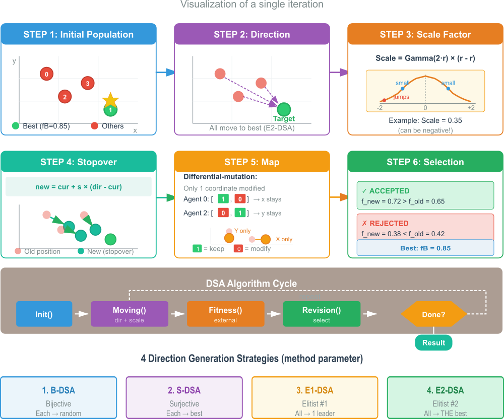
Figure 1. DSA algorithm workflow diagram

The illustration shows the six steps of a single iteration: the initial population consists of points in the search space; the best point is marked in green; direction generation (E2-DSA), where all individuals move toward the best individual, is shown with directional arrows; Scale Factor — a graph showing the distribution of step sizes: many small steps and infrequent large jumps; Stopover calculation — the formula and a visualization of points moving to new positions; application of the Map, showing how the mask determines which coordinates to change (0=change, 1=keep); and Selection — examples of accepting and rejecting new positions.

The algorithm cycle is also shown — the sequence of calls: Init → Moving → CalcFitness → Revision → repeat — and, at the end, the four direction strategies, with brief descriptions of the B-DSA, S-DSA, E1-DSA, and E2-DSA methods.

Let's move on to writing the pseudocode for the algorithm.

1. INITIALIZATION
FOR each individual i = 1..popSize
x[i] = a random point within bounds
f[i] = compute fitness(x[i])
END FOR
xBest = best individual
fBest = best fitness

2. MAIN LOOP (iter = 1..maxIter)

2.1. Save the current state
xPrev = x
fPrev = f

2.2. FOR each individual i

a) Select a direction (depends on the method):
- B-DSA (1): direction = a different random individual
- S-DSA (2): direction = a randomly selected top individual
- E1-DSA (3): direction = one randomly selected leader (the same for all)
- E2-DSA (4): direction = the best individual (the same for all)

b) Compute the scale:
scale = Gamma(2·rand) × (rand - rand)

c) Compute the intermediate position:
stopover[d] = xPrev[i][d] + scale × (direction[d] - xPrev[i][d])
for all coordinates d = 1..dim

d) Generate a Mutation Map:
prob = random number [0, 1]
IF prob < p1 THEN
// Random-mutation #1: each coordinate has a ~50% chance of changing
map[d] = randomly 0 or 1
ELSE IF prob > (1 - p1) THEN
// Differential-mutation: only ONE coordinate
randomCoord = random index
map[d] = 1 for all d except randomCoord
map[randomCoord] = 0
ELSE
// Random-mutation #2: multiple coordinates
numModify = ceil(rand × p2 × dim)
map = all 1
select numModify random coordinates and set them to 0
END IF

e) Apply the Mutation Map:
FOR d = 1..dim
IF map[d] == 0 THEN
x[i][d] = stopover[d] // change
ELSE
x[i][d] = xPrev[i][d] // keep the old value
END IF
END FOR

f) Check the bounds:
FOR d = 1..dim
IF x[i][d] is outside the bounds THEN
IF rand < 0.5 THEN
x[i][d] = a random value within the bounds
ELSE
x[i][d] = the nearest boundary
END IF
END IF
END FOR

END FOR

2.3. Compute the fitness for all new positions
FOR i = 1..popSize
f[i] = fitness(x[i])
END FOR

2.4. Selection (greedy selection)
FOR i = 1..popSize
IF f[i] > fPrev[i] THEN
// accept the new position (already in x[i])
ELSE
// revert to the old one
x[i] = xPrev[i]
f[i] = fPrev[i]
END IF
END FOR

2.5. Update the global best
IF max(f) > fBest THEN
xBest = x[index of max(f)]
fBest = max(f)
END IF

END LOOP

RETURN xBest, fBest

Now we can move on to the actual implementation in code. A data structure named "S_DSA_Map" is used to manage information about "active" objects associated with a specific number of "coordinates." The main part of this structure is an array called "active." The size of this array is not fixed at declaration, allowing it to be adjusted dynamically. Essentially, each element of this array will correspond to a single "coordinate." The information stored in each "active" element is initially set to zero, which implies an inactive state by default.

The structure also contains an Init function, which is used for initialization. When the function is called, it is passed a number representing the total number of "coordinates"; it then resizes the "active" array so that it has the appropriate size—that is, the number of elements will equal the value passed for "coordinates." After that, it ensures that all elements of this array are set to zero.

//—————————————————————————————————————— ——————————————————————————————
struct S_DSA_Map
{
    int active []; // map of active individuals for each coordinate

    void Init (int coords)
    {
      ArrayResize (active, coords);
      ArrayInitialize (active, 0);
    }
};
//————————————————————————————————————————————————————————————————————

The C_AO_DSA class is derived from the base class C_AO and is designed to implement the Differential Search Algorithm.

Algorithm parameters:

• popSize — the population size.
• method — selects the Differential Search method to use. The default value is 1, which corresponds to the B-DSA method. Possible values: 1 (B-DSA), 2 (S-DSA), 3 (E1-DSA), 4 (E2-DSA).
• p1 — a control parameter for the mutation strategy.
• p2 — the second control parameter for the mutation strategy.

The class constructor initializes the internal "params" structure, which stores the names and current values of "popSize", "method", "p1", and "p2". The "SetParams" method is responsible for updating the values of the parameters listed above based on the "params" structure. After receiving the new values, the method checks and adjusts the parameters to ensure they are within the acceptable limits.

Main Methods:

• Init — initializes the algorithm. It takes the search ranges and search step, as well as the number of epochs (iterations),
• Moving — is responsible for moving and updating objects within the algorithm,
• Revision — is used to revise or correct solutions.

Private data and methods:

• direction — an array that stores information about "agents" (population members) and their directions,
• mapArray — an array of S_DSA_Map structures which, as described in the previous section, are used to manage the state of active elements by coordinate,
• InitializePopulation — a method for creating the initial population,
• GenerateDirection — a method for generating agent movement directions, depending on the selected methodType,
• GenerateMap — a method for generating the S_DSA_Map map,
• GenerateScaleFactor — a method for generating the Scale Factor used in mutations,
• GammaRandom — a method for generating random numbers from a Gamma distribution with specified shape and scale parameters,
• BoundaryControl — a method for handling out-of-bounds coordinates for a given agent, using the specified index.

Overall, C_AO_DSA is an implementation of the Differential Search Algorithm that allows various aspects of its operation to be configured, such as the population size, the mutation method used, and the control-variable parameters.

//————————————————————————————————————————————————————————————————————
class C_AO_DSA : public C_AO
{
  public:
  ~C_AO_DSA () { }

  C_AO_DSA ()
  {
    ao_name = "DSA";
    ao_desc = "Differential Search Algorithm";
    ao_link = "https://www.mql5.com/en/articles/20346";

    popSize = 50;
    method  = 1;    // 1-B-DSA, 2-S-DSA, 3-E1-DSA, 4-E2-DSA
    p1      = 0.3;  // mutation strategy control [0.0, 0.3]
    p2      = 0.3;  // mutation strategy control [0.0, 0.3]

    ArrayResize (params, 4);
    params [0].name = "popSize";  params [0].val = popSize;
    params [1].name = "method";   params [1].val = method;
    params [2].name = "p1";       params [2].val = p1;
    params [3].name = "p2";       params [3].val = p2;
  }

  void SetParams ()
  {
    popSize = (int)params [0].val;
    method  = (int)params [1].val;
    p1      = params [2].val;
    p2      = params [3].val;

    if (method < 1) method = 1;
    if (method > 4) method = 4;
    if (p1 < 0.0) p1 = 0.0;
    if (p1 > 0.3) p1 = 0.3;
    if (p2 < 0.0) p2 = 0.0;
    if (p2 > 0.3) p2 = 0.3;
  }

  bool Init (const double &rangeMinP  [],
             const double &rangeMaxP  [],
             const double &rangeStepP [],
             const int     epochsP);

  void Moving   ();
  void Revision ();

  //------------------------------------------------------------------
  int    method;
  double p1;
  double p2;

  private: //---------------------------------------------------------
  S_AO_Agent direction [];
  S_DSA_Map  mapArray  [];

  void   InitializePopulation  ();
  void   GenerateDirection     (int methodType);
  void   GenerateMap           ();
  double GenerateScaleFactor   ();
  double GammaRandom           (double shape, double scale);
  void   BoundaryControl       (int idx);
};
//————————————————————————————————————————————————————————————————————

The Init initialization function for the C_AO_DSA class. First, the StandardInit function is called; it performs the general initialization steps required for all algorithms based on C_AO. If this basic initialization fails, the class function immediately terminates and returns false.

Initializing the direction array. An array named "direction" is created, whose size is determined by the popSize variable (population size). Next, the element's own Init method is called for each element in the "direction" array. In this case, each element is passed the "coords" value, which represents the number of "coordinates" used in the algorithm.

Initializing the array of maps. An array named mapArray is created, also with a size equal to popSize. As with the "direction" array, the Init method is called for each element in mapArray. Here, too, the "coords" value is passed, allowing the S_DSA_Map structure to be configured correctly for each element. If all previous steps have been completed successfully, the Init function returns true.

//————————————————————————————————————————————————————————————————————
bool C_AO_DSA::Init (const double &rangeMinP  [],
                     const double &rangeMaxP  [],
                     const double &rangeStepP [],
                     const int     epochsP)
{
  if (!StandardInit (rangeMinP, rangeMaxP, rangeStepP)) return false;

  //------------------------------------------------------------------
  ArrayResize (direction, popSize);
  for (int i = 0; i < popSize; i++) direction [i].Init (coords);

  ArrayResize (mapArray, popSize);
  for (int i = 0; i < popSize; i++) mapArray [i].Init (coords);

  return true;
}
//————————————————————————————————————————————————————————————————————

The Moving method of the C_AO_DSA class is responsible for the main logic governing the movement of agents (population representatives) during the operation of the Differential Search Algorithm.

Population initialization (on the first iteration). If the "revision" flag is set to false (indicating that this is the first iteration), the InitializePopulation method is called to create the initial population of agents. After that, the "revision" flag is set to true, and execution of the method ends until the next iteration.

Saving the current state. At each subsequent iteration (when "revision" is 'true'), the current coordinates "c" and their corresponding fitness function values "f" are saved for each agent. The saved coordinates are stored in the cP array (previous coordinates), and the fitness values are stored in fP.

Generating the direction and the Scale Factor. The "GenerateDirection" method is called; it determines the "direction" for each agent. The specific direction-generation strategy is selected based on the "method" parameter. Next, the GenerateScaleFactor method is called to obtain the Scale Factor. This coefficient affects the magnitude of the displacement step.

Calculating a new position (preliminary). A new preliminary position is calculated for each agent and each coordinate. The new coordinate is calculated as: (previous coordinate) + (Scale Factor) * (difference between the direction and the previous coordinate). This stage essentially forms a new “candidate” position.

Generating the active/passive coordinate map. The GenerateMap method is called. As mentioned earlier, this method creates the mapArray structure that specifies, for each agent, which coordinates are “active” (requiring an update) and which are “passive” (must remain unchanged).

Position adjustment taking the map and bounds into account. For each agent, the map of active/passive coordinates is checked. If a coordinate is marked as “active,” its new position is reset to the value of the previous coordinate. In other words, this coordinate is not updated. If the coordinate is “passive,” the new value calculated in step 4 is retained. After adjusting the coordinates, the BoundaryControl method is called for each agent to ensure that all coordinates are within the permissible search bounds.

Thus, the Moving method simulates a single step in the evolution of a population, in which agents generate new potential positions, which are then modified and constrained according to the specified rules and algorithm parameters.

//————————————————————————————————————————————————————————————————————
void C_AO_DSA::Moving ()
{
  //------------------------------------------------------------------
  // First iteration: initializing the population
  if (!revision)
  {
    InitializePopulation ();
    revision = true;
    return;
  }

  //------------------------------------------------------------------
  // Store the current coordinates and fitness in cP and fP
  for (int i = 0; i < popSize; i++)
  {
    ArrayCopy (a [i].cP, a [i].c, 0, 0, coords);
    a [i].fP = a [i].f;
  }

  //------------------------------------------------------------------
  // Generating a direction based on cP (old coordinates)
  GenerateDirection (method);

  // Generating the Scale Factor
  double scale = GenerateScaleFactor ();

  //------------------------------------------------------------------
  // Calculate the stopover site and store it in c
  for (int i = 0; i < popSize; i++)
  {
    for (int c = 0; c < coords; c++)
    {
      double diff = direction [i].c [c] - a [i].cP [c];
      a [i].c [c] = a [i].cP [c] + scale * diff;
    }
  }

  //------------------------------------------------------------------
  // Generating the active/passive coordinate map
  GenerateMap ();

  //------------------------------------------------------------------
  // Restore coordinates where map > 0 (keep the original ones)
  for (int i = 0; i < popSize; i++)
  {
    for (int c = 0; c < coords; c++)
    {
      if (mapArray [i].active [c] > 0)
      {
        a [i].c [c] = a [i].cP [c];
      }
    }

    // Boundary control
    BoundaryControl (i);
  }
}
//————————————————————————————————————————————————————————————————————

The InitializePopulation method of the C_AO_DSA class. Its main task is to create and initialize the initial state of the agent population. The method iterates through each agent in the population, from the first to the last (the number of agents is determined by the variable popSize). For each agent, the method processes all of its coordinates sequentially. For each coordinate of the current agent, a random number is generated within the specified range (from rangeMin to rangeMax). This is done using the u.RNDfromCI function.

The resulting random value is then additionally adjusted using the u.SeInDiSp function. The adjusted value is assigned to the corresponding coordinate "c" of the current agent. Thus, InitializePopulation is responsible for generating an initial, random, yet valid configuration for each agent in the population (within the specified ranges and steps), thereby preparing the population for the algorithm's subsequent operation.

//————————————————————————————————————————————————————————————————————
void C_AO_DSA::InitializePopulation ()
{
  for (int i = 0; i < popSize; i++)
  {
    for (int c = 0; c < coords; c++)
    {
      a [i].c [c] = u.RNDfromCI (rangeMin [c], rangeMax [c]);
      a [i].c [c] = u.SeInDiSp (a [i].c [c], rangeMin [c], rangeMax [c], rangeStep [c]);
    }
  }
}
//————————————————————————————————————————————————————————————————————

The next method of the C_AO_DSA class, GenerateDirection, is responsible for determining the direction vector for each agent in the population. The method takes a methodType parameter, which determines which particular direction-generation algorithm will be used. Various direction generation strategies (depending on methodType):

Type 1: B-DSA (Bijective) — random permutation:

• An array of indices corresponding to all agents is created.
• The Fisher-Yates shuffle algorithm is used to randomly reorder these indices.
• For each agent in the population, its "direction" vector is set equal to the coordinates of the agent whose index ended up in the corresponding position after the random permutation.
• Objective: each agent "looks" toward another random agent.

Type 2: S-DSA (Surjective) — toward randomly selected top individuals:

• An array of agent indices is created.
• Agents are sorted in descending order of their fitness value "fP".
• For each agent, the number of “top” agents (topCount) from which a candidate will be selected is determined at random. One agent is randomly selected from this group of “top” agents. The direction vector of the current agent is set equal to the previous coordinates (cP) of the selected “top” agent.
• Objective: agents “move toward” randomly selected more successful agents.

Type 3: E1-DSA (Elitist #1) — toward one randomly selected top individual:

• As with Type 2, agents are sorted in descending order of fitness.
• A group of “top” agents (topCount) is determined at random.
• From this group, one random “top” agent is selected.
• All agents in the population set their direction vector equal to the previous coordinates of this single selected “top” agent.
• Objective: all agents “orient themselves” toward a randomly selected agent that is still among the top individuals.

Type 4: E2-DSA (Elitist #2) — toward the best individual:

• The agent with the highest fitness (bestIdx) is found.
• All agents in the population set their direction vector equal to the previous coordinates of this overall best agent.
• Objective: all agents “copy” or “move toward” the strongest member of the population.

Thus, the GenerateDirection method implements various strategies for “information exchange” or “orientation” among agents, allowing the algorithm to explore the search space based on information about the best or randomly selected members of the population.

//————————————————————————————————————————————————————————————————————
void C_AO_DSA::GenerateDirection (int methodType)
{
  // Use cP (old coordinates) to generate the direction
  switch (methodType)
  {
    case 1: // B-DSA (Bijective) — random permutation
    {
      int indices [];
      ArrayResize (indices, popSize);
      for (int i = 0; i < popSize; i++) indices [i] = i;

      // Fisher-Yates shuffle
      for (int i = popSize - 1; i > 0; i--)
      {
        int j = u.RNDminusOne (i + 1);
        int temp = indices [i];
        indices [i] = indices [j];
        indices [j] = temp;
      }

      for (int i = 0; i < popSize; i++)
      {
        ArrayCopy (direction [i].c, a [indices [i]].cP, 0, 0, coords);
      }
      break;
    }

    case 2: // S-DSA (Surjective) — toward randomly selected top individuals
    {
      int sortedIdx [];
      ArrayResize (sortedIdx, popSize);
      for (int i = 0; i < popSize; i++) sortedIdx [i] = i;

      // Sort by fP (old fitness) in descending order
      for (int i = 0; i < popSize - 1; i++)
      {
        for (int j = 0; j < popSize - i - 1; j++)
        {
          if (a [sortedIdx [j]].fP < a [sortedIdx [j + 1]].fP)
          {
            int temp = sortedIdx [j];
            sortedIdx [j] = sortedIdx [j + 1];
            sortedIdx [j + 1] = temp;
          }
        }
      }

      for (int i = 0; i < popSize; i++)
      {
        int topCount = (int)MathCeil (u.RNDfromCI (0.0, 1.0) * popSize);
        if (topCount < 1) topCount = 1;
        int selectedIdx = sortedIdx [u.RNDminusOne (topCount)];
        ArrayCopy (direction [i].c, a [selectedIdx].cP, 0, 0, coords);
      }
      break;
    }

    case 3: // E1-DSA (Elitist #1) — toward one randomly selected top individual
    {
      int sortedIdx [];
      ArrayResize (sortedIdx, popSize);
      for (int i = 0; i < popSize; i++) sortedIdx [i] = i;

      for (int i = 0; i < popSize - 1; i++)
      {
        for (int j = 0; j < popSize - i - 1; j++)
        {
          if (a [sortedIdx [j]].fP < a [sortedIdx [j + 1]].fP)
          {
            int temp = sortedIdx [j];
            sortedIdx [j] = sortedIdx [j + 1];
            sortedIdx [j + 1] = temp;
          }
        }
      }

      int topCount = (int)MathCeil (u.RNDfromCI (0.0, 1.0) * popSize);
      if (topCount < 1) topCount = 1;
      int bestIdx = sortedIdx [u.RNDminusOne (topCount)];

      for (int i = 0; i < popSize; i++)
      {
        ArrayCopy (direction [i].c, a [bestIdx].cP, 0, 0, coords);
      }
      break;
    }

    case 4: // E2-DSA (Elitist #2) — toward the best individual
    {
      int bestIdx = 0;
      double bestFit = a [0].fP;
      for (int i = 1; i < popSize; i++)
      {
        if (a [i].fP > bestFit)
        {
          bestFit = a [i].fP;
          bestIdx = i;
        }
      }

      for (int i = 0; i < popSize; i++)
      {
        ArrayCopy (direction [i].c, a [bestIdx].cP, 0, 0, coords);
      }
      break;
    }
  }
}
//————————————————————————————————————————————————————————————————————

The GenerateMap method is designed to create a Mutation Map that will be applied to the population of agents. This map determines which coordinates of which agents will be subject to changes. Two random variables are generated. Before specific mutations are determined, all positions in the map are set to "0".

The main condition for selecting a mutation strategy. Two random numbers, each generated in the range [0.0, 1.0], are compared. The probability that the main condition is met (i.e., "true") is 0.5, which means that the choice between the two main branches of the algorithm (the first with two subbranches, "Random-mutation #1" and "Differential-mutation," and the second, "Random-mutation #2") is made randomly with a 50% probability.

Case 1: Random-mutation #1. For each agent and each of its coordinates, another random number is generated. If it is less than another random number, then mapArray[i].active[c] is set to "1". Again, comparing two random numbers means that each individual coordinate is activated with a probability of 0.5. Goal: to randomly activate individual coordinates in different agents, marking them for mutation.

• Differential-mutation (otherwise): For each agent, "mapArray[i].active" is initialized entirely to "1" (all coordinates are active for mutation). Then, one coordinate (modifyCoord) is selected at random for each agent, and for this specific coordinate, "mapArray[i].active[modifyCoord]" is set to "0" (disabled). Goal: only one randomly selected coordinate mutates for each agent.

Case 2: Random-mutation #2. The number of coordinates to mutate (numModify) is determined for each agent. It depends on "p2_iter" and the total number of coordinates. The number is limited to a reasonable range (from "1" to "coords"). For each agent, the entire mapArray[i].active array is initialized to "1". Then, coordinates are selected at random "numModify" times, and mapArray[i].active[modifyCoord] is set to "0" for those coordinates. Goal: each agent mutates a fixed (but random) number of coordinates.

The GenerateMap method is responsible for setting mutation masks. It generates the mapArray structure that contains information for each agent about which of its coordinates should be changed. The algorithm offers several different strategies for creating this mask, allowing the process of exploring the search space to vary — from randomly applying mutations to individual coordinates to more targeted changes.

//————————————————————————————————————————————————————————————————————
void C_AO_DSA::GenerateMap ()
{
  double p1_iter = u.RNDfromCI (0.0, p1);
  double p2_iter = u.RNDfromCI (0.0, p2);

  for (int i = 0; i < popSize; i++)
  {
    ArrayInitialize (mapArray [i].active, 0);
  }

  if (u.RNDfromCI (0.0, 1.0) < u.RNDfromCI (0.0, 1.0))
  {
    if (u.RNDfromCI (0.0, 1.0) < p1_iter)
    {
      // Random-mutation #1
      for (int i = 0; i < popSize; i++)
      {
        for (int c = 0; c < coords; c++)
        {
          if (u.RNDfromCI (0.0, 1.0) < u.RNDfromCI (0.0, 1.0))
          {
            mapArray [i].active [c] = 1;
          }
        }
      }
    }
    else
    {
      // Differential-mutation
      for (int i = 0; i < popSize; i++)
      {
        ArrayInitialize (mapArray [i].active, 1);
        int modifyCoord = u.RNDminusOne (coords);
        mapArray [i].active [modifyCoord] = 0;
      }
    }
  }
  else
  {
    // Random-mutation #2
    int numModify = (int)MathCeil (p2_iter * coords);
    if (numModify < 1) numModify = 1;
    if (numModify > coords) numModify = coords;

    for (int i = 0; i < popSize; i++)
    {
      ArrayInitialize (mapArray [i].active, 1);

      for (int k = 0; k < numModify; k++)
      {
        int modifyCoord = u.RNDminusOne (coords);
        mapArray [i].active [modifyCoord] = 0;
      }
    }
  }
}
//————————————————————————————————————————————————————————————————————

The GenerateScaleFactor function of the C_AO_DSA class generates the Scale Factor. This method generates a Scale Factor that is used to control the "length" of the step taken by the agents. Using the Gamma distribution and random numbers allows us to introduce variation in the magnitude and direction of this step, which can help the algorithm explore the search space more effectively, avoid local minima, and find the global optimum.

• rand1 — affects the "shape" of the Gamma distribution, making it "broader" or "narrower" depending on its value.
• gamma_val — a random positive number whose distribution depends on rand1.
• rand2 - rand3 — determines the sign and relative magnitude of the Scale Factor. The result can be positive (if rand2 > rand3) or negative (if rand2 < rand3).

Ultimately, GenerateScaleFactor returns a Scale Factor that is "random in magnitude and direction" and is applied to the direction vector to form the step vector.

//————————————————————————————————————————————————————————————————————
double C_AO_DSA::GenerateScaleFactor ()
{
  double rand1 = u.RNDfromCI (0.0, 1.0);
  double rand2 = u.RNDfromCI (0.0, 1.0);
  double rand3 = u.RNDfromCI (0.0, 1.0);

  double shape = 2.0 * rand1;
  double gamma_val = GammaRandom (shape, 1.0);

  return gamma_val * (rand2 - rand3);
}
//————————————————————————————————————————————————————————————————————

Next comes the implementation of the "GammaRandom" function, which generates random numbers distributed according to the Gamma distribution. The Gamma distribution is an important probability distribution; it models the waiting time until a certain number of independent events have occurred, each occurring at a certain average rate. It has two parameters:

• shape — defines the shape of the distribution,
• scale — determines how "stretched" the distribution is.

In DSA, it is used to create a pseudo-stable random walk—a specific movement pattern characterized by frequent small steps and occasional large leaps. The GammaRandom function implements the Marsaglia–Tsang algorithm (2000), the acceptance-rejection method (Rejection Sampling).

Purpose of GammaRandom: this helper function for DSA requires generating numbers from a Gamma distribution. As mentioned earlier, in DSA, the Gamma distribution can be used to generate the Scale Factor, which makes it possible to control the magnitude and direction of agents' steps in the search space.

We recursively call the function with (shape + 1), then multiply the result by a random number raised to the power of (1/shape). This reduces the result and shifts the distribution toward zero. Case 2: shape ≥ 1. Acceptance-rejection method: compute the auxiliary constants "d" and "c" from "shape," generate a candidate "x" from the normal distribution N(0,1), and compute v = (1 + c·x)³. We check whether the candidate can be accepted. Quick test: compare a random number with a simple expression. Exact test: compare logarithms. If it is accepted, return (d·v·scale). If it is rejected, repeat starting from step 2. Safeguards:

• minimum shape = 0.01 (to avoid division by zero)
• check that v > 0 before cubing
• protection against log(0)
• maximum of 100 iterations (in case of bad luck)

The result is a positive number, where small values occur frequently, large values occur rarely, and the mean value is ≈ shape × scale.

//————————————————————————————————————————————————————————————————————
double C_AO_DSA::GammaRandom (double shape, double scale)
{
  if (shape <= 0.0) return 1.0;
  if (shape < 0.01) shape = 0.01;

  if (shape < 1.0)
  {
    double gamma = GammaRandom (1.0 + shape, scale);
    double u_rand = u.RNDfromCI (1e-10, 1.0);
    return gamma * MathPow (u_rand, 1.0 / shape);
  }

  double d = shape - 1.0 / 3.0;
  double c = 1.0 / MathSqrt (9.0 * d);

  int maxIter = 100;
  int iter = 0;

  while (iter < maxIter)
  {
    iter++;
    double x, v;

    do
    {
      x = u.GaussDistribution (0.0, 1.0, -10.0, 10.0);
      v = 1.0 + c * x;
    }
    while (v <= 0.0);

    v = v * v * v;
    double u_rand = u.RNDfromCI (1e-10, 1.0);
    double x_sq = x * x;

    if (u_rand < 1.0 - 0.0331 * x_sq * x_sq)
    {
      return scale * d * v;
    }

    if (MathLog (u_rand) < 0.5 * x_sq + d * (1.0 - v + MathLog (v)))
    {
      return scale * d * v;
    }
  }

  return scale * d;
}
//————————————————————————————————————————————————————————————————————

The BoundaryControl function is intended to perform boundary control for a specific agent. Its purpose is to ensure that each agent's coordinates remain within the allowed range.

Why is this kind of boundary handling necessary?

In optimization algorithms, especially population-based ones (such as DSA), agents move through the search space. When calculating an agent's new position, its coordinates can often fall outside the permissible range defined by the problem formulation. The BoundaryControl function ensures that:

• agents remain within a physically or logically valid region;
• incorrect calculations in subsequent iterations that could be caused by going out of bounds are prevented;
• The use of probabilistic replacement (u.RNDfromCI (rangeMin [c], rangeMax [c])) instead of simple “reflection” or “clipping” can help prevent “clusters” of agents from forming right at the boundaries, thereby promoting a more thorough exploration of the search space.

//————————————————————————————————————————————————————————————————————
void C_AO_DSA::BoundaryControl (int idx)
{
  for (int c = 0; c < coords; c++)
  {
    if (a [idx].c [c] < rangeMin [c])
    {
      if (u.RNDprobab () < 0.5)
      {
        a [idx].c [c] = u.RNDfromCI (rangeMin [c], rangeMax [c]);
      }
      else
      {
        a [idx].c [c] = rangeMin [c];
      }
    }

    if (a [idx].c [c] > rangeMax [c])
    {
      if (u.RNDprobab () < 0.5)
      {
        a [idx].c [c] = u.RNDfromCI (rangeMin [c], rangeMax [c]);
      }
      else
      {
        a [idx].c [c] = rangeMax [c];
      }
    }

    a [idx].c [c] = u.SeInDiSp (a [idx].c [c], rangeMin [c], rangeMax [c], rangeStep [c]);
  }
}
//————————————————————————————————————————————————————————————————————

The Revision function performs two main steps after new agent positions are generated in the algorithm: selection to determine which of the new positions will be retained, and updating the global best solution.

Step 1: Selection (Evaluation of New Solutions). For each agent in the population, the value of its new position (how “good” or “fit” it is) is compared with the value of its previous position. If the new position turns out to be no better (that is, either equal in quality or worse) than the previous one, the agent returns to its old, more advantageous position. This means that only the steps that led to an improvement are retained. If the agent did not have a valid previous position, this condition does not apply.

Step 2: Updating the global best. After all agents have determined which position to keep, the function searches all current agent positions for the one with the best quality (the highest fitness score). This quality is then compared with the best quality recorded over the entire runtime of the algorithm. If the current best position in the population outperforms the previously found overall best solution, it becomes the new global best solution, and the location of this best solution is stored.

//————————————————————————————————————————————————————————————————————
void C_AO_DSA::Revision ()
{
  //------------------------------------------------------------------
  // Selection: accept only if the new fitness is better than the old one
  for (int i = 0; i < popSize; i++)
  {
    // If the new fitness (f) is NOT better than the old one (fP), restore the previous position
    if (a [i].f <= a [i].fP && a [i].fP != -DBL_MAX)
    {
      a [i].f = a [i].fP;
      ArrayCopy (a [i].c, a [i].cP, 0, 0, coords);
    }
  }

  //------------------------------------------------------------------
  // Updating the Global Best
  int bestIdx = 0;
  double bestFit = a [0].f;

  for (int i = 1; i < popSize; i++)
  {
    if (a [i].f > bestFit)
    {
      bestFit = a [i].f;
      bestIdx = i;
    }
  }

  if (bestFit > fB)
  {
    fB = bestFit;
    ArrayCopy (cB, a [bestIdx].c, 0, 0, coords);
  }
}
//————————————————————————————————————————————————————————————————————

Test results

The results show the capabilities of all four methods available in the settings. As you can see, the second method scores highest when each individual moves toward a randomly selected solution from the top-N best solutions.

DSA|Differential Search Algorithm|50.0|1.0|0.3|0.3|
=============================
5 Hilly's; Func runs: 10000; result: 0.6982999549366771
25 Hilly's; Func runs: 10000; result: 0.4112441157981344
500 Hilly's; Func runs: 10000; result: 0.26639110224055546
=============================
5 Forest's; Func runs: 10000; result: 0.7546811566849957
25 Forest's; Func runs: 10000; result: 0.33583122216029415
500 Forest's; Func runs: 10000; result: 0.18324446089620824
=============================
5 Megacity's; Func runs: 10000; result: 0.5538461538461539
25 Megacity's; Func runs: 10000; result: 0.2156923076923077
500 Megacity's; Func runs: 10000; result: 0.10643076923077019
=============================
Overall score: 3.52566 (39.17%)

1 (B-DSA)

DSA|Differential Search Algorithm|50.0|2.0|0.3|0.3|
=============================
5 Hilly's; Func runs: 10000; result: 0.75651834013058
25 Hilly's; Func runs: 10000; result: 0.420539560652641
500 Hilly's; Func runs: 10000; result: 0.2673297720453783
=============================
5 Forest's; Func runs: 10000; result: 0.8226119802254519
25 Forest's; Func runs: 10000; result: 0.3408987112971432
500 Forest's; Func runs: 10000; result: 0.18471282959506144
=============================
5 Megacity's; Func runs: 10000; result: 0.5323076923076923
25 Megacity's; Func runs: 10000; result: 0.22153846153846152
500 Megacity's; Func runs: 10000; result: 0.10521538461538557
=============================
Overall score: 3.65167 (40.57%)

2 (S-DSA)

DSA|Differential Search Algorithm|50.0|3.0|0.3|0.3|
=============================
5 Hilly's; Func runs: 10000; result: 0.704394194121553
25 Hilly's; Func runs: 10000; result: 0.415864841547213
500 Hilly's; Func runs: 10000; result: 0.26675670523279044
=============================
5 Forest's; Func runs: 10000; result: 0.8200531047825427
25 Forest's; Func runs: 10000; result: 0.3345381783754753
500 Forest's; Func runs: 10000; result: 0.18518322851491886
=============================
5 Megacity's; Func runs: 10000; result: 0.49846153846153846
25 Megacity's; Func runs: 10000; result: 0.21846153846153848
500 Megacity's; Func runs: 10000; result: 0.1064307692307701
=============================
Overall score: 3.55014 (39.45%)

3 (E1-DSA)

DSA|Differential Search Algorithm|50.0|4.0|0.3|0.3|
=============================
5 Hilly's; Func runs: 10000; result: 0.7184577016736993
25 Hilly's; Func runs: 10000; result: 0.4114617093550586
500 Hilly's; Func runs: 10000; result: 0.2650947599954659
=============================
5 Forest's; Func runs: 10000; result: 0.8159647894070122
25 Forest's; Func runs: 10000; result: 0.3307842077432657
500 Forest's; Func runs: 10000; result: 0.18482144990330598
=============================
5 Megacity's; Func runs: 10000; result: 0.4800000000000001
25 Megacity's; Func runs: 10000; result: 0.20769230769230776
500 Megacity's; Func runs: 10000; result: 0.10500000000000091
=============================
Overall score: 3.51928 (39.10%)

4 (E2-DSA)

In the visualization, the DSA algorithm behaves fairly compactly, without much scatter; the convergence quality on low-dimensional functions could be better.

DSA on the Hilly test function

DSA on the Forest test function

DSA on the Megacity test function

For problems involving standard test functions, the algorithm performs well, showing good convergence and a small spread of results.

DSA on the standard Paraboloid test function

DSA on the standard test function GoldsteinPrice

The DSA algorithm is included in the ranking table for informational purposes.

Description	Hilly			Hilly Final	Forest			Forest Final	Megacity (discrete)			Megacity Final	Final Result	% of MAX
	10 p (5 F)	50 p (25 F)	1,000 p (500 F)		10 p (5 F)	50 p (25 F)	1,000 p (500 F)		10 p (5 F)	50 p (25 F)	1,000 p (500 F)
dingo_optimization_algorithm_M	0.47968	0.45367	0.46369	1.39704	0.94145	0.87909	0.91454	2.73508	0.78615	0.86061	0.84805	2.49481	6.627	73.63
across-neighborhood search	0.94948	0.84776	0.43857	2.23581	1.00000	0.92334	0.39988	2.32323	0.70923	0.63477	0.23091	1.57491	6.134	68.15
code lock algorithm (JOO)	0.95345	0.87107	0.37590	2.20042	0.98942	0.91709	0.31642	2.22294	0.79692	0.69385	0.19303	1.68380	6.107	67.86
animal migration optimization M	0.90358	0.84317	0.46284	2.20959	0.99001	0.92436	0.46598	2.38034	0.56769	0.59132	0.23773	1.39675	5.987	66.52
(P+O) evolution strategies	0.92256	0.88101	0.40021	2.20379	0.97750	0.87490	0.31945	2.17185	0.67385	0.62985	0.18634	1.49003	5.866	65.17
comet tail algorithm (JOO)	0.95346	0.86319	0.27770	2.09435	0.99794	0.85740	0.33949	2.19484	0.88769	0.56431	0.10512	1.55712	5.846	64.96
time-evolution travel algorithm (JOO)	0.91362	0.82349	0.31990	2.05701	0.97096	0.89532	0.29324	2.15952	0.73462	0.68569	0.16021	1.58052	5.797	64.41
stochastic diffusion search M	0.93066	0.85445	0.39476	2.17988	0.99983	0.89244	0.19619	2.08846	0.72333	0.61100	0.10670	1.44103	5.709	63.44
billiards optimization algorithm M	0.95757	0.82599	0.25235	2.03590	1.00000	0.90036	0.30502	2.20538	0.73538	0.52523	0.09563	1.35625	5.598	62.19
archery algorithm M	0.91744	0.70876	0.42160	2.04780	0.92527	0.75802	0.35328	2.03657	0.67385	0.55200	0.23738	1.46323	5.548	61.64
evolution of social groups (JOO)	0.99906	0.79654	0.35056	2.14616	1.00000	0.82863	0.13102	1.95965	0.82333	0.55300	0.04725	1.42358	5.529	61.44
simulated isotropic annealing (JOO)	0.95784	0.84264	0.41465	2.21513	0.98239	0.79586	0.20507	1.98332	0.68667	0.49300	0.09053	1.27020	5.469	60.76
extremal_optimization_M	0.76166	0.77242	0.31747	1.85155	0.99999	0.76751	0.23527	2.00277	0.74769	0.53969	0.14249	1.42987	5.284	58.71
biiogeography-based optimization	0.94912	0.69456	0.35031	1.99399	0.93820	0.67365	0.25682	1.86867	0.74615	0.48277	0.17369	1.40261	5.265	58.50
artificial cooperative search	0.75547	0.74744	0.30407	1.80698	1.00000	0.88861	0.22413	2.11274	0.69077	0.48185	0.13322	1.30583	5.226	58.06
dialectical algorithm	0.86183	0.70033	0.33724	1.89940	0.98163	0.72772	0.28718	1.99653	0.70308	0.45292	0.16367	1.31967	5.216	57.95
black hole algorithm M	0.75236	0.76675	0.34583	1.86493	0.93593	0.80152	0.27177	2.00923	0.65077	0.51646	0.15472	1.32195	5.196	57.73
anarchy society optimization	0.84872	0.74646	0.31465	1.90983	0.96148	0.79150	0.23803	1.99101	0.57077	0.54062	0.16614	1.27752	5.178	57.54
royal flush optimization (JOO)	0.83361	0.73742	0.34629	1.91733	0.89424	0.73824	0.24098	1.87346	0.63154	0.50292	0.16421	1.29867	5.089	56.55
atomic orbital search M	0.80232	0.70449	0.31021	1.81702	0.85660	0.69451	0.21996	1.77107	0.74615	0.52862	0.14358	1.41835	5.006	55.63
turtle shell evolution algorithm (JOO)	0.96798	0.64480	0.29672	1.90949	0.99449	0.61981	0.22708	1.84139	0.69077	0.42646	0.13598	1.25322	5.004	55.60
backtracking_search_algorithm	0.97309	0.54534	0.29098	1.80941	0.99999	0.58543	0.21747	1.80289	0.84769	0.36953	0.12978	1.34700	4.959	55.10
differential evolution	0.95044	0.61674	0.30308	1.87026	0.95317	0.78896	0.16652	1.90865	0.78667	0.36033	0.02953	1.17653	4.955	55.06
successful restaurateur algorithm (JOO)	0.96883	0.63455	0.29217	1.89555	0.94637	0.55506	0.19124	1.69267	0.74923	0.44031	0.12526	1.31480	4.903	54.48
bonobo_optimizer	0.77565	0.63805	0.32908	1.74278	0.88088	0.76344	0.25573	1.90005	0.61077	0.49846	0.14246	1.25169	4.895	54.38
chemical reaction optimization	0.94629	0.66112	0.29853	1.90593	0.87906	0.58422	0.21146	1.67473	0.75846	0.42646	0.12686	1.31178	4.892	54.36
blood inheritance optimization (JOO)	0.81568	0.65336	0.30877	1.77781	0.89937	0.65319	0.21760	1.77016	0.67846	0.47631	0.13902	1.29378	4.842	53.80
dream_optimization_algorithm	0.85556	0.70085	0.37280	1.92921	0.73421	0.48905	0.24147	1.46473	0.77231	0.47354	0.18561	1.43146	4.825	53.62
bird swarm algorithm	0.89306	0.64900	0.26250	1.80455	0.92420	0.71121	0.24939	1.88479	0.69385	0.32615	0.10012	1.12012	4.809	53.44
dolphin_echolocation_algorithm	0.75995	0.67572	0.34171	1.77738	0.89582	0.64223	0.23941	1.77746	0.61538	0.44031	0.15115	1.20684	4.762	52.91
harmony search	0.86509	0.68782	0.32527	1.87818	0.99999	0.68002	0.09590	1.77592	0.62000	0.42267	0.05458	1.09725	4.751	52.79
saplings sowing and growing	0.77839	0.64925	0.39543	1.82308	0.85973	0.62467	0.17429	1.65869	0.64667	0.44133	0.10598	1.19398	4.676	51.95
bacterial chemotaxis optimization M	0.75953	0.62268	0.31483	1.69704	0.89378	0.61339	0.22542	1.73259	0.65385	0.42092	0.14435	1.21912	4.649	51.65
african buffalo optimization	0.83337	0.62247	0.29964	1.75548	0.92170	0.58618	0.19723	1.70511	0.61000	0.43154	0.13225	1.17378	4.634	51.49
(PO) Evolution Strategies	0.79025	0.62647	0.42935	1.84606	0.87616	0.60943	0.19591	1.68151	0.59000	0.37933	0.11322	1.08255	4.610	51.22
fractal-based algorithm	0.79000	0.65134	0.28965	1.73099	0.87158	0.56823	0.18877	1.62858	0.61077	0.46062	0.12398	1.19537	4.555	50.61
tabu search M	0.87795	0.61431	0.29104	1.78330	0.92885	0.51844	0.19054	1.63783	0.61077	0.38215	0.12157	1.11449	4.536	50.40
brain storm optimization	0.93736	0.57616	0.29688	1.81041	0.93131	0.55866	0.23537	1.72534	0.55231	0.29077	0.11914	0.96222	4.498	49.98
whale optimization algorithm M	0.84521	0.56298	0.26263	1.67081	0.93100	0.52278	0.16365	1.61743	0.66308	0.41138	0.11357	1.18803	4.476	49.74
artificial electric field algorithm	0.87700	0.61753	0.25235	1.74688	0.92729	0.72698	0.18064	1.83490	0.66615	0.11631	0.09508	0.87754	4.459	49.55
artificial ecosystem-based optimization algorithm	0.91380	0.46713	0.26470	1.64563	0.90223	0.43705	0.21400	1.55327	0.66154	0.30800	0.28563	1.25517	4.454	49.49
camel algorithm M	0.78684	0.56042	0.35133	1.69859	0.82772	0.56041	0.24336	1.63149	0.64846	0.33092	0.13418	1.11356	4.444	49.37
ant colony optimization M	0.88190	0.66127	0.30377	1.84693	0.85873	0.58680	0.15051	1.59604	0.59667	0.37333	0.02472	0.99472	4.438	49.31
covariance matrix adaptation evolution strategy	0.76258	0.72089	0.00000	1.48347	0.82056	0.79616	0.00000	1.61672	0.75846	0.49077	0.00000	1.24923	4.349	48.33
duelist algorithm	0.92782	0.53778	0.27792	1.74352	0.86957	0.47536	0.18193	1.52686	0.62153	0.33569	0.11715	1.07437	4.345	48.28
differential search algorithm	0.75651	0.42054	0.26733	1.44438	0.82261	0.34090	0.18471	1.34822	0.53231	0.22154	0.10521	0.85906	3.652	40.57
random walk	0.48754	0.32159	0.25781	1.06694	0.37554	0.21944	0.15877	0.75375	0.27969	0.14917	0.09847	0.52734	2.348	26.09

Conclusions

The Differential Search Algorithm (DSA) demonstrates average performance on optimization test problems. When using the S-DSA strategy, in which each individual moves toward a randomly selected solution from the top-N best solutions, the algorithm achieves just over 40% performance relative to the reference values. This strategy provides the best balance between exploration of the search space and exploitation of the solutions found. The other three direction-generation strategies show slightly worse results, lagging behind by no more than 1.5%, which indicates that the algorithm is relatively robust with respect to parameter selection.

Unfortunately, when tested on low-, medium-, and high-dimensional problems, the algorithm does not score high enough to make it into the ranking table of the best optimization methods. Nevertheless, DSA performs consistently and reliably, confidently handling standard test functions and producing solutions of acceptable quality.

DSA's average performance can be attributed to several factors. First, while using a Gamma distribution to generate the step size provides a theoretically sound pseudo-stable random walk, in practice it can result in insufficiently aggressive exploration of the search space during the early iterations. Second, the mechanism of partially changing coordinates via a Mutation Map — by altering only one or a few coordinates per iteration — slows convergence in multidimensional spaces, where simultaneous adjustment of multiple variables is required to reach the optimum. Third, greedy selection — in which any worsening of a solution is rejected — can lead to premature convergence and getting stuck in local optima.

The algorithm’s strengths include its conceptual simplicity and the intuitive metaphor of superorganism migration, a small number of tunable parameters, consistent results across different settings, and the guaranteed preservation of the best solutions found through elitist selection.

This algorithm may be recommended for practical problems where maximum accuracy is not required, but ease of implementation and predictable behavior are important. DSA is well suited for preliminary optimization followed by refinement using other methods, for problems with a limited computational budget where result stability is important, and for educational purposes as an illustrative example of a metaheuristic algorithm with clearly separated exploration and exploitation components.

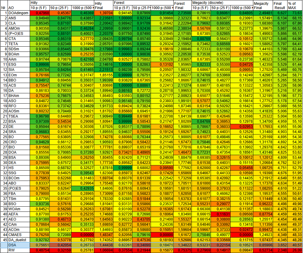
Figure 2. Color coding of algorithms for the corresponding tests

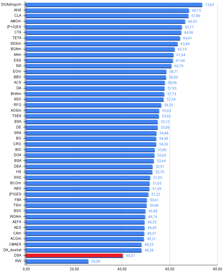
Figure 3. Histogram of the algorithm test results (on a scale from 0 to 100; the higher the score, the better, where 100 is the maximum possible theoretical result; the archive contains a script for calculating the ranking table)

Pros and cons of DSA:

Pros:

1. Fast.
2. Small variation in results across runs.
3. Best results for medium- and high-dimensional functions.

Cons:

1. Weaker results on low-dimensional functions.

An archive containing the current versions of the algorithm code is attached to the article. The author of this article is not responsible for the absolute accuracy of the descriptions of the canonical algorithms; many of them have been modified to improve their search capabilities. The conclusions and judgments presented in the articles are based on the results of the experiments conducted.

• GitHub: https://github.com/JQSakaJoo/Population-optimization-algorithms-MQL5

Programs used in this article

#	Name	Type	Description
1	#C_AO.mqh	Include file	Parent class for population-based optimization algorithms
2	#C_AO_enum.mqh	Include file	Enumeration of population-based optimization algorithms
3	TestFunctions.mqh	Include file	Test function library
4	TestStandFunctions.mqh	Include file	Test bench function library
5	Utilities.mqh	Include file	Utility function library
6	CalculationTestResults.mqh	Include file	Script for computing results for the comparison table
7	Testing AOs.mq5	Script	Unified test bench for all population-based optimization algorithms
8	Simple use of population optimization algorithms.mq5	Script	A simple example of using population-based optimization algorithms without visualization
9	Test_AO_DSA.mq5	Script	Test bench for DSA