Online Linear Regression with Recursive Least Squares in MQL5: A Parameter-Free Adaptive Trend Estimator

Introduction

Linear regression is a useful way to measure the current slope of a market and project where price is heading. Most MQL5 implementations recalculate the full regression from scratch on every bar. For a small lookback window this is barely noticeable, but on tick charts, large lookback windows, or multi-symbol scanners running several indicators simultaneously, the cost adds up quickly.

Recursive Least Squares (RLS) solves this by maintaining the regression state incrementally. Instead of rebuilding the calculation from all historical observations each bar, the filter stores a compact state and updates it using only the newest data point. The update cost stays constant regardless of how much history the chart holds.

This article builds a complete MQL5 implementation. The result is two indicators that update in constant time per bar:

• A forecast line drawn directly on the price chart, showing where the model expects price to be one bar ahead
• A slope histogram in a separate subwindow, showing the strength and direction of the current adaptive trend

Both are driven by a single reusable class, CRLSRegression, which can be dropped into any indicator or EA that needs a lightweight, adaptive linear trend estimate.

Section 1: Why Not Recompute OLS Every Bar?

A standard rolling-window OLS indicator rebuilds its normal matrix from all observations in the window on every bar. For a 200-bar window, that is 200 accumulation steps before a single coefficient is produced. For a 1000-bar window it is 1000 steps — five times the work, and this entire calculation is discarded and rebuilt when the next bar arrives, even though 999 of the 1000 observations are unchanged.

This is an O(n) cost per bar, where n is the window size. Summed across a full chart history it becomes O(n²). On a daily chart with a modest lookback this rarely matters. On a tick chart, or when the same logic runs across dozens of symbols, it becomes a real bottleneck.

RLS replaces the full rebuild with a fixed-cost update. The filter stores the current coefficient estimate and a compact representation of the inverse covariance matrix and updates both using only the newest observation via the Sherman-Morrison rank-1 formula. The update requires the same small number of scalar operations whether the filter has seen 20 bars or 200,000. That is O(1) per bar, independent of history length.

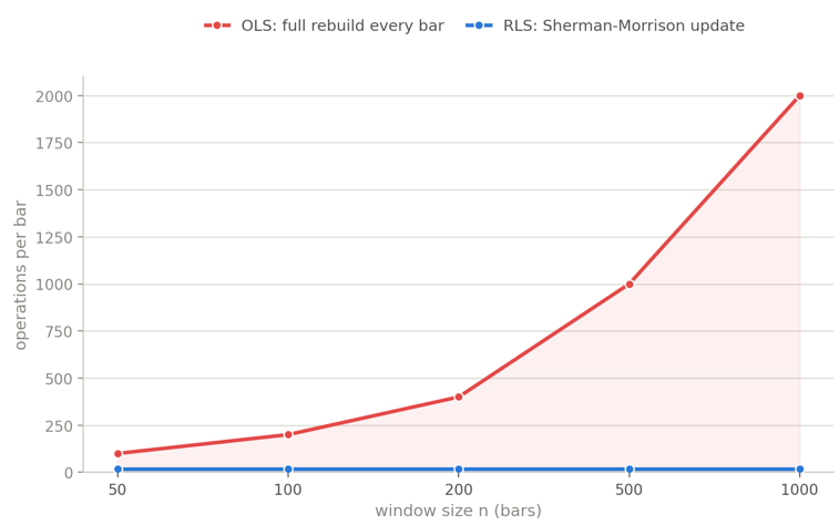
Per-bar operation count as window size grows: OLS's full rebuild scales linearly with n, while RLS's Sherman-Morrison update stays constant.

Section 2: What the Trader Gets

Before the mathematics, here is what the two indicators actually show and when they are useful:

• Forecast line (RLSForecast.mq5): This is the model's estimate of where price will be on the next bar, drawn directly on the candles. When the forecast line begins curling upward after a period of decline, the model is detecting a shift in the short-term trend before the price has moved far enough to confirm it visually. When the line is nearly flat, the model sees no meaningful directional slope. When price consistently trades above or below the forecast, the market is moving faster than the current forgetting factor allows the model to track.
• Slope histogram (RLSSlope.mq5): This shows the rate of change of price per bar under the exponentially weighted objective, displayed as a bar chart in a separate subwindow. Green bars indicate an upward slope, red bars indicate a downward slope. Rising positive values mean the trend is accelerating. Positive values that begin falling toward zero suggest momentum is fading. A sign change — a green bar following a red, or vice versa — is the model's signal of a possible regime change.

When this is useful:

• Detecting trend acceleration or deceleration before it is obvious on the candles
• Filtering entries in trend-following systems by requiring a positive slope above a threshold
• Identifying early momentum exhaustion when slope values start declining while price is still rising
• Combining with breakout logic to confirm that the directional move has a measured rate of change behind it

These are not standalone entry signals. They are measurements of trend slope and direction that augment whatever decision logic the trader already uses.

Section 3: The Mathematics of RLS (Useful but Optional)

If you are primarily interested in the practical implementation, you can skim this section and move on to Section 4.

The model

The underlying model is a linear trend in time: y_t = θ₀ + θ₁ · t + ε_t, where θ₀ is the intercept and θ₁ is the slope — the rate of price change per bar. Written in vector form with x_t = [1, t]ᵀ and θ = [θ₀, θ₁]ᵀ, this is y_t = xᵀ_t · θ. Standard OLS finds the θ that minimizes the sum of squared residuals across all n observations, requiring a matrix build and inversion at cost O(n). RLS finds the same class of solution adaptively, at O(1) per bar.

The forgetting factor

RLS weights historical observations exponentially by their age. An observation k bars old receives weight λ^k, where λ is the forgetting factor between 0 and 1. When λ = 1 every bar has equal weight, equivalent to standard OLS over all available history. When λ < 1, recent bars dominate and old ones fade gradually — a soft, exponentially decaying window rather than a hard cutoff.

A practical way to think about λ is the effective window formula:

effective_n = 1 / (1 − λ)

The table below shows the effective window for common values of λ, which can serve as a starting point when choosing a forgetting factor based on a familiar lookback length.

λ	Effective window (bars)
0.95	20
0.98	50
0.99	100
0.995	200

A good starting point for daily-bar indicators is λ = 0.98, which behaves like a 50-bar recency-weighted regression while reacting to new data on every bar rather than only after the window has fully rolled past a change.

Choosing λ too close to 1.0 produces a slow, nearly static estimate. Choosing it too close to 0.0 produces a noisy estimate dominated by the last one or two bars. For most trading applications the range 0.95 to 0.99 is the practical space to explore, with 0.98 as a reasonable default.

The recursive update

The three formulas that make RLS work are:

K_t = P_{t-1} · x_t / (λ + xᵀ_t · P_{t-1} · x_t)     — gain vector
P_t = (P_{t-1} − K_t · xᵀ_t · P_{t-1}) / λ           — covariance update
θ_t = θ_{t-1} + K_t · (y_t − xᵀ_t · θ_{t-1})         — coefficient update

In plain terms:

• The gain vector K_t determines how much the new bar changes the current estimate. When the filter is uncertain, the gain is large and new data has a strong effect. When the pattern has stabilized, the gain is smaller and the estimate moves less.
• The innovation (y_t − xᵀ_t · θ_{t-1}) is the prediction error: how far off the previous model was on this new bar. The coefficient update applies the gain vector scaled by that error.
• The P update shrinks to reflect the information gained from the new observation, then expands slightly via the 1/λ factor to keep the filter sensitive to future changes rather than becoming overconfident and unresponsive.

Initialization

The filter starts with θ = [0, 0]ᵀ and P = δ · I, where δ is a large scalar (typically 1000) and I is the 2×2 identity matrix. A large initial δ means high initial uncertainty, which produces a large early gain — the first few observations move the estimate quickly toward a reasonable value. A small δ would behave as if the filter had already seen many bars confirming θ = [0, 0]ᵀ, causing slow adaptation during warm-up regardless of what the price data shows.

The 1-step-ahead forecast

Once θ is estimated through bar t, the forecast for the next bar is:

ŷ_{t+1} = θ₀_t + θ₁_t · (t + 1)

This is what RLSForecast.mq5 plots, written one bar forward of the bar that produced the estimate.

Section 4: Implementation — RLSRegression.mqh

CRLSRegression is the statistical engine behind both indicators. It maintains the coefficient estimate and inverse covariance matrix and applies the Sherman-Morrison update on each new observation. It has no knowledge of indicator buffers, chart bars, or MQL5's OnCalculate lifecycle. This keeps it independently testable and reusable in any indicator or EA context.

A note on matrix storage

The 2×2 inverse covariance matrix P is stored as four individual double members — m_P00, m_P01, m_P10, m_P11 — rather than as a 2D array. For a fixed two-feature model this keeps every line of the update formula directly readable without index arithmetic, and eliminates a class of off-by-one errors that are easy to introduce and hard to spot in matrix indexing code. This is a deliberate special-case choice and would not generalize to an arbitrary number of regressors.

//+------------------------------------------------------------------+
//|                                                RLSRegression.mqh |
//+------------------------------------------------------------------+
#ifndef RLSREGRESSION_MQH
#define RLSREGRESSION_MQH

//+------------------------------------------------------------------+
//| Class CRLSRegression                                             |
//| Purpose: maintains a recursively updated linear regression of    |
//| y on a time index, using the Sherman-Morrison rank-1 update      |
//| with a forgetting factor for non-stationary tracking.            |
//+------------------------------------------------------------------+
class CRLSRegression
  {
private:
   double            m_theta0;
   double            m_theta1;
   double            m_P00;
   double            m_P01;
   double            m_P10;
   double            m_P11;
   double            m_lambda;
   double            m_delta;
   int               m_obs_count;
   int               m_min_obs;

public:
                     CRLSRegression(void);
                    ~CRLSRegression(void);

   void              Init(double lambda,double delta,int min_obs);
   void              Reset(void);
   void              Update(double y,double t_index);
   double            GetSlope(void) const;
   double            GetIntercept(void) const;
   double            Forecast(double t_index) const;
   bool              IsValid(void) const;
   int               GetObsCount(void) const;
  };

Constructor

The constructor sets working defaults so a CRLSRegression object is usable immediately without a mandatory Init call:

//+------------------------------------------------------------------+
//| Constructor                                                      |
//+------------------------------------------------------------------+
CRLSRegression::CRLSRegression(void)
  {
   m_lambda=0.98;
   m_delta=1000.0;
   m_min_obs=20;
   m_obs_count=0;
   m_theta0=0.0;
   m_theta1=0.0;
   m_P00=m_delta;
   m_P01=0.0;
   m_P10=0.0;
   m_P11=m_delta;
  }

Init()

Init() stores the three configurable parameters and calls Reset so the coefficient and covariance state is always consistent with the assigned delta:

//+------------------------------------------------------------------+
//| Configure the filter's parameters and reset its state            |
//+------------------------------------------------------------------+
void CRLSRegression::Init(double lambda,double delta,int min_obs)
  {
   m_lambda=lambda;
   m_delta=delta;
   m_min_obs=min_obs;
   Reset();
  }

Reset()

Reset() restores θ to [0,0] and P to δ·I without touching λ, δ, or min_obs — useful both from Init and from an indicator's OnCalculate when prev_calculated == 0 signals that the entire history must be reprocessed:

//+------------------------------------------------------------------+
//| Reset theta to zero and P to delta times the identity matrix     |
//+------------------------------------------------------------------+
void CRLSRegression::Reset(void)
  {
   m_theta0=0.0;
   m_theta1=0.0;
   m_P00=m_delta;
   m_P01=0.0;
   m_P10=0.0;
   m_P11=m_delta;
   m_obs_count=0;
  }

Update()

The Update() method is where the Sherman-Morrison formula runs. Each block maps to one line of the mathematics from Section 3:

//+------------------------------------------------------------------+
//| Apply the Sherman-Morrison rank-1 RLS update for one new         |
//| observation y at time index t_index                              |
//+------------------------------------------------------------------+
void CRLSRegression::Update(double y,double t_index)
  {
//--- feature vector is x = [1, t_index]
   double x0=1.0;
   double x1=t_index;

//--- P_{t-1} * x_t  (a 2x1 vector, computed from the 2x2 P and x)
   double Px0=m_P00*x0+m_P01*x1;
   double Px1=m_P10*x0+m_P11*x1;

//--- denominator: lambda + x_t' * P_{t-1} * x_t
   double denom=m_lambda+(x0*Px0+x1*Px1);

//--- gain vector K_t = (P_{t-1} * x_t) / denom
   double K0=Px0/denom;
   double K1=Px1/denom;

//--- innovation: prediction error using the previous theta
   double y_hat=m_theta0*x0+m_theta1*x1;
   double innovation=y-y_hat;

//--- coefficient update: theta_t = theta_{t-1} + K_t * innovation
   m_theta0=m_theta0+K0*innovation;
   m_theta1=m_theta1+K1*innovation;

//--- x_t' * P_{t-1}  (a 1x2 row vector)
   double xP0=x0*m_P00+x1*m_P10;
   double xP1=x0*m_P01+x1*m_P11;

//--- P update: P_t = (P_{t-1} - K_t * (x_t' * P_{t-1})) / lambda
   double newP00=(m_P00-K0*xP0)/m_lambda;
   double newP01=(m_P01-K0*xP1)/m_lambda;
   double newP10=(m_P10-K1*xP0)/m_lambda;
   double newP11=(m_P11-K1*xP1)/m_lambda;

   m_P00=newP00;
   m_P01=newP01;
   m_P10=newP10;
   m_P11=newP11;

   m_obs_count++;
  }

Three implementation details worth noting. The innovation uses the pre-update θ — the coefficient update comes before the P update precisely because of this. The row vector xP is computed independently from Px rather than reused as its transpose. P is mathematically symmetric, but floating-point rounding can cause m_P01 and m_P10 to drift apart over long runs. Computing both explicitly avoids compounding that error. All four new P values are computed into temporaries before any assignment, so no earlier-updated entry contaminates a later one within the same call.

GetSlope()

//+------------------------------------------------------------------+
//| Accessor: current slope estimate (theta1)                        |
//+------------------------------------------------------------------+
double CRLSRegression::GetSlope(void) const
  {
   return(m_theta1);
  }

GetSlope() returns the current estimate of θ₁, the rate of change of y per unit of the time index, as described in Section 2's discussion of the slope as a trend detector.

GetIntercept()

//+------------------------------------------------------------------+
//| Accessor: current intercept estimate (theta0)                    |
//+------------------------------------------------------------------+
double CRLSRegression::GetIntercept(void) const
  {
   return(m_theta0);
  }

GetIntercept() returns the current estimate of θ₀. On its own this value is rarely meaningful for trading, since it represents the model's fitted value at time index zero rather than at the current bar. It is exposed for completeness and because Forecast() depends on it.

Forecast()

//+------------------------------------------------------------------+
//| Compute the model's forecast at a given time index               |
//+------------------------------------------------------------------+
double CRLSRegression::Forecast(double t_index) const
  {
   return(m_theta0+m_theta1*t_index);
  }

Forecast() evaluates the current linear model θ₀ + θ₁ · t_index at whatever time index is supplied, implementing the 1-step-ahead forecast formula from Section 3 when called with t_index equal to one more than the index of the most recent observation. Because the method takes the time index as a parameter rather than always assuming "one bar ahead" internally, it can also be used to evaluate the current fitted value at the most recent bar itself, which is useful for the verification script in Section 8.

IsValid()

//+------------------------------------------------------------------+
//| True once at least m_min_obs observations have been processed    |
//+------------------------------------------------------------------+
bool CRLSRegression::IsValid(void) const
  {
   return(m_obs_count>=m_min_obs);
  }

IsValid() reports whether the filter has processed enough observations to be considered past its warm-up period, comparing m_obs_count against the configured m_min_obs threshold. This is the check both of this article's indicators use to decide whether to write a real value or EMPTY_VALUE into their output buffers for a given bar, preventing an under-determined early estimate from being displayed.

GetObsCount()

//+------------------------------------------------------------------+
//| Accessor: number of observations processed so far                |
//+------------------------------------------------------------------+
int CRLSRegression::GetObsCount(void) const
  {
   return(m_obs_count);
  }

GetObsCount() exposes the raw observation counter directly, which the verification script in Section 8 uses to check IsValid()'s behavior at specific, known counts, and which a calling indicator could use for diagnostic logging. This completes RLSRegression.mqh. The usage pattern is straightforward: call Init() once, then Update() on each new observation, and read GetSlope(), GetIntercept(), Forecast(), and IsValid() as needed. Both indicator files in Sections 6 and 7 follow this exact sequence.

Section 5: Indicator Buffer Architecture

MQL5 does not allow a single compiled indicator to draw some plots in the chart window and others in a subwindow, the #property indicator_chart_window / indicator_separate_window setting applies to the entire indicator file.

This matters here because the forecast and the slope live on completely different numeric scales. The forecast is a price, sitting near whatever the current symbol's price level is. The slope is a rate of change per bar, typically several orders of magnitude smaller. If both were plotted on the same axis, the slope histogram would be compressed to an invisible sliver near zero against the price-scale axis.

The solution is two separate indicator files, each with its own auto-scaled axis. RLSForecast.mq5 is a chart-window indicator drawing the forecast line at price scale. RLSSlope.mq5 is a subwindow indicator drawing the slope histogram at its own natural scale. Both include the same RLSRegression.mqh and drive their own CRLSRegression instance. Their outputs always agree because the algorithm is deterministic.

The slope histogram uses DRAW_COLOR_HISTOGRAM, which pairs a data buffer with a parallel color-index buffer. Writing 0 into the color buffer selects the positive-slope color and writing 1 selects the negative-slope color, giving each bar the correct green or red rendering automatically.

Section 6: Implementation — RLSForecast.mq5

RLSForecast.mq5 is the chart-window half of this article's indicator pair. Its sole output is the 1-step-ahead forecast, drawn as a line directly on the price candles where its price-scale values are directly comparable to the close.

The property block declares this as a chart-window indicator with one buffer and one plot, drawn as a DRAW_LINE in a dark orange chosen to stand out against typical candle colors. The three inputs — InpLambda, InpDelta, InpMinObs — expose the filter's tunable parameters, with defaults matching the values recommended in Section 3. 

g_ForecastBuffer[] is the single indicator buffer, and g_rls is this file's own CRLSRegression instance, entirely independent of the instance driven by RLSSlope.mq5.

//+------------------------------------------------------------------+
//|                                                  RLSForecast.mq5 |
//+------------------------------------------------------------------+

#property indicator_chart_window
#property indicator_buffers 1
#property indicator_plots   1

#property indicator_label1  "RLS Forecast"
#property indicator_type1   DRAW_LINE
#property indicator_color1  clrDarkOrange
#property indicator_width1  2

//--- Include
#include <RLSRegression\RLSRegression.mqh>

//--- Inputs
input double InpLambda = 0.98;    // InpLambda
input double InpDelta  = 1000.0;  // InpDelta
input int    InpMinObs = 20;      // InpMinObs

double g_ForecastBuffer[];

CRLSRegression g_rls;

OnInit() wires the buffer, sets EMPTY_VALUE as the no-data marker, assigns the short name, and initializes the filter:

//+------------------------------------------------------------------+
//| Custom indicator initialization function                         |
//+------------------------------------------------------------------+
int OnInit(void)
  {
   SetIndexBuffer(0,g_ForecastBuffer,INDICATOR_DATA);
   ArraySetAsSeries(g_ForecastBuffer,false);
   PlotIndexSetDouble(0,PLOT_EMPTY_VALUE,EMPTY_VALUE);

   IndicatorSetString(INDICATOR_SHORTNAME,
                      StringFormat("RLS Forecast (lambda=%.2f)",InpLambda));

   g_rls.Init(InpLambda,InpDelta,InpMinObs);

   PrintFormat("RLSForecast initialized: lambda=%.4f, delta=%.2f, min_obs=%d",
               InpLambda,InpDelta,InpMinObs);

   return(INIT_SUCCEEDED);
  }

OnCalculate() follows the standard MQL5 incremental pattern. When prev_calculated == 0 the filter resets and the full history is reprocessed from bar 0. Otherwise only the most recently formed bar is updated, and the filter's accumulated state is left intact:

//+------------------------------------------------------------------+
//| Custom indicator iteration function                              |
//+------------------------------------------------------------------+
int OnCalculate(const int rates_total,
                const int prev_calculated,
                const datetime &time[],
                const double &open[],
                const double &high[],
                const double &low[],
                const double &close[],
                const long &tick_volume[],
                const long &volume[],
                const int &spread[])
  {
   int start;

   if(prev_calculated==0)
     {
      g_rls.Reset();
      start=0;
      for(int i=0; i<rates_total; i++)
         g_ForecastBuffer[i]=EMPTY_VALUE;
     }
   else
     {
      start=prev_calculated-1;
     }

   for(int i=start; i<rates_total; i++)
     {
      double t_index=(double)i;

      g_rls.Update(close[i],t_index);

      if(g_rls.IsValid())
        {
         if(i+1<rates_total)
            g_ForecastBuffer[i+1]=g_rls.Forecast(t_index+1.0);
        }
      else
        {
         g_ForecastBuffer[i]=EMPTY_VALUE;
        }
     }

   return(rates_total);
  }

The forecast is written into g_ForecastBuffer[i+1] — one bar forward of the bar whose close produced the estimate. This visually shifts the forecast one bar forward within the available history, so on the chart it appears alongside the next bar rather than the bar whose close produced it. On the live bar, the entry is skipped entirely because the i+1 < rates_total guard is not satisfied.

Section 7: Implementation — RLSSlope.mq5

RLSSlope.mq5 is the subwindow half of this article's indicator pair. Its sole output is the slope, rendered as a signed color histogram in its own subwindow, free to auto-scale to the small magnitude of a per-bar price-change rate without a price-scale series distorting the axis.

//+------------------------------------------------------------------+
//|                                                     RLSSlope.mq5 |
//+------------------------------------------------------------------+

#property indicator_separate_window
#property indicator_buffers 3
#property indicator_plots   1

#property indicator_label1  "RLS Slope"
#property indicator_type1   DRAW_COLOR_HISTOGRAM
#property indicator_color1  clrSeaGreen,clrCrimson
#property indicator_width1  2

//--- Include
#include <RLSRegression\RLSRegression.mqh>

//--- Inputs
input double InpLambda = 0.98;    // InpLambda
input double InpDelta  = 1000.0;  // InpDelta
input int    InpMinObs = 20;      // InpMinObs

double g_SlopeBuffer[];
double g_SlopeColorBuffer[];
double g_InterceptBuffer[];

CRLSRegression g_rls;

Three buffers are declared: the slope data buffer, its paired color-index buffer, and an intercept buffer registered as INDICATOR_CALCULATIONS — computed but not drawn, visible in the Data Window for diagnostics.

//+------------------------------------------------------------------+
//| Custom indicator initialization function                         |
//+------------------------------------------------------------------+
int OnInit(void)
  {
   SetIndexBuffer(0,g_SlopeBuffer,INDICATOR_DATA);
   SetIndexBuffer(1,g_SlopeColorBuffer,INDICATOR_COLOR_INDEX);
   SetIndexBuffer(2,g_InterceptBuffer,INDICATOR_CALCULATIONS);

   ArraySetAsSeries(g_SlopeBuffer,false);
   ArraySetAsSeries(g_SlopeColorBuffer,false);
   ArraySetAsSeries(g_InterceptBuffer,false);

   PlotIndexSetDouble(0,PLOT_EMPTY_VALUE,EMPTY_VALUE);
   PlotIndexSetInteger(0,PLOT_COLOR_INDEXES,2);

   IndicatorSetString(INDICATOR_SHORTNAME,
                      StringFormat("RLS Slope (lambda=%.2f)",InpLambda));

   g_rls.Init(InpLambda,InpDelta,InpMinObs);

   PrintFormat("RLSSlope initialized: lambda=%.4f, delta=%.2f, min_obs=%d",
               InpLambda,InpDelta,InpMinObs);

   return(INIT_SUCCEEDED);
  }

OnCalculate() follows the same incremental pattern as RLSForecast. The only difference is what gets written per bar: the slope value and a color index of 0 (green) or 1 (red) depending on its sign, plus the intercept into the calculation buffer:

//+------------------------------------------------------------------+
//| Custom indicator iteration function                              |
//+------------------------------------------------------------------+
int OnCalculate(const int rates_total,
                const int prev_calculated,
                const datetime &time[],
                const double &open[],
                const double &high[],
                const double &low[],
                const double &close[],
                const long &tick_volume[],
                const long &volume[],
                const int &spread[])
  {
   int start;

   if(prev_calculated==0)
     {
      g_rls.Reset();
      start=0;
      for(int i=0; i<rates_total; i++)
        {
         g_SlopeBuffer[i]=EMPTY_VALUE;
         g_SlopeColorBuffer[i]=0.0;
         g_InterceptBuffer[i]=EMPTY_VALUE;
        }
     }
   else
     {
      start=prev_calculated-1;
     }

   for(int i=start; i<rates_total; i++)
     {
      double t_index=(double)i;

      g_rls.Update(close[i],t_index);

      if(g_rls.IsValid())
        {
         double slope=g_rls.GetSlope();

         g_SlopeBuffer[i]=slope;
         g_SlopeColorBuffer[i]=(slope>=0.0) ? 0.0 : 1.0;
         g_InterceptBuffer[i]=g_rls.GetIntercept();
        }
      else
        {
         g_SlopeBuffer[i]=EMPTY_VALUE;
         g_SlopeColorBuffer[i]=0.0;
         g_InterceptBuffer[i]=EMPTY_VALUE;
        }
     }

   return(rates_total);
  }

RLSForecast (orange, main chart) and RLSSlope (histogram, subwindow) on EURUSD H1 — the forecast lags the sharp late rally while the slope's sign flips positive only after it begins.

Section 8: How to Read the Indicators

Forecast line

When the forecast begins curving upward after a downward sequence, the model is detecting an early shift in slope. When the forecast is nearly flat and price is moving, the model's effective window is too long relative to the move's speed — consider a lower λ. When price consistently trades above a rising forecast, the market is accelerating faster than the model tracks, which itself is information about the move's strength.

Slope histogram

Green bars mean the model's current slope estimate is positive; red bars mean it is negative. What matters more than the color is the trajectory:

• Rising green bars signal trend acceleration.
• Green bars that begin shrinking toward zero signal fading momentum even while price may still be rising.
• A bar near zero following a sequence of same-sign bars is the earliest sign the weighted balance of recent price changes is reversing.
• A full sign change — red following green or vice versa — is the model's clearest signal of a regime shift, though like all such signals it appears after the fact relative to the actual turning bar.

Tuning λ

The forgetting factor is the most important parameter. A smaller λ makes the indicators react faster but introduces more noise in ranging markets. A larger λ smooths the output but delays the response to genuine trend changes. A useful starting point is to match λ to the effective window the strategy already uses. For a 50-bar window, start with λ = 0.98 and adjust based on how quickly the slope histogram reflects moves that are obvious on the candles.

Section 9: Verification

TestRLS.mq5 feeds a noise-free linear sequence into CRLSRegression and checks that the recovered slope and intercept converge to the values that generated the sequence.

//+------------------------------------------------------------------+
//|                                                     TestRLS.mq5  |
//+------------------------------------------------------------------+

#include <RLSRegression\RLSRegression.mqh>

#define ASSERT(cond,msg) { if(cond) Print("PASS: ",msg); else Print("FAIL: ",msg); }

//+------------------------------------------------------------------+
//| Script program start function                                    |
//+------------------------------------------------------------------+
void OnStart(void)
  {
   CRLSRegression rls;
   rls.Init(0.98,1000.0,20);

   for(int i=0; i<5; i++)
     {
      double y=2.0+3.0*(double)i;
      rls.Update(y,(double)i);
     }

   ASSERT(rls.IsValid()==false,
          "filter is not valid after only 5 observations (min_obs=20)");

   for(int i=5; i<50; i++)
     {
      double y=2.0+3.0*(double)i;
      rls.Update(y,(double)i);
     }

   double slope=rls.GetSlope();
   double intercept=rls.GetIntercept();

   ASSERT(MathAbs(slope-3.0)<0.01,
          StringFormat("slope converges to 3.0 after 50 observations (got %.6f)",slope));
   ASSERT(MathAbs(intercept-2.0)<0.5,
          StringFormat("intercept converges near 2.0 after 50 observations (got %.6f)",intercept));

   double forecast=rls.Forecast(51.0);
   ASSERT(MathAbs(forecast-155.0)<0.5,
          StringFormat("Forecast(51) is approximately 155.0 (got %.6f)",forecast));

   PrintFormat("Final state after 50 observations: theta0=%.6f, theta1=%.6f, obs_count=%d",
               intercept,slope,rls.GetObsCount());
  }
//+------------------------------------------------------------------+

The slope tolerance is tight (0.01) because the slope is well-determined by the trend across all 50 observations. The intercept tolerance is wider (0.5) because θ₀ represents the model's fitted value at t = 0, a coordinate seen only once at the very start of warm-up when the estimate was still poor. This reflects the running time-index convention where t_index = i is passed directly from the bar array index, not a defect in the update itself.

Running the script prints three PASS lines to the Experts tab. A FAIL on the slope line points to Update(); a FAIL on the intercept points to the same; a FAIL on the forecast points to Forecast().

Section 10: RLS vs. Fixed-Window OLS

RLS with λ = 0.98 and fixed-window OLS with a 50-bar lookback cover roughly the same amount of recent history but distribute that weight differently. OLS assigns every bar in the window equal weight and drops each bar the instant it ages out. RLS weights the newest bar most heavily and decays older bars continuously. There is no sudden discontinuity 50 bars after a sharp change — the influence fades gradually rather than cutting off abruptly.

The practical difference is most visible near trend changes. RLS begins adjusting to a new trend immediately because the newest bar always carries the highest weight. Fixed-window OLS carries the old trend until enough new bars enter the window to outweigh the bars still representing the prior regime.

Fixed-window OLS is preferable when the window length itself has external meaning — a fixed reporting period, for instance. RLS is preferable when the goal is continuous adaptive tracking of a trend that cannot be assumed stationary, and when the O(1) per-bar cost is a practical requirement.

Section 11: Limitations

Not equivalent to fixed-window OLS: As Section 10 describes, RLS with a forgetting factor and hard-windowed OLS weight history differently. They will produce different slopes and forecasts, particularly in the bars following a sharp trend change.

Numerical drift over long runs: Each call to Update applies floating-point subtraction and division to the P matrix entries. Over thousands of bars, small rounding errors accumulate. P can gradually lose positive-definiteness or develop small asymmetries between m_P01 and m_P10. The Reset method is public specifically so calling code can invoke it on a schedule — for instance, once per session or every several thousand bars — without modifying the class itself. Neither indicator in this article calls Reset on a periodic schedule by default, since the appropriate interval is application-specific.

Fixed two-feature model: The implementation is built for an intercept and a single time index and does not generalize to additional regressors without restructuring the scalar matrix storage described in Section 4.

No prediction interval: The forecast is a point estimate only. The innovation computed inside Update could in principle support a running variance estimate for a confidence band, but this is not implemented here.

Two indicator files, two computations: Attaching both indicators to the same chart means the regression runs twice per bar. Given the O(1) cost this is negligible, but it is an architectural tradeoff made for the visual benefit of correct axis scaling on each output.

Conclusion

This article builds a complete MQL5 implementation of recursive least squares for adaptive trend estimation. The CRLSRegression class applies the Sherman-Morrison rank-1 update in explicit scalar form, maintaining an exponentially weighted coefficient estimate that updates in a fixed number of operations per bar regardless of how long the chart history grows. RLSForecast.mq5 plots the 1-step-ahead forecast directly on price. RLSSlope.mq5 plots the slope as a signed color histogram in its own correctly-scaled subwindow.

The practical payoffs are three. The update cost is O(1) per bar, replacing the O(n) rebuild of a rolling OLS indicator. The forgetting factor λ controls adaptiveness through a single, interpretable parameter tied to an effective window length via 1/(1−λ). The visualization architecture gives each output the axis scale it needs, keeping the forecast and slope histogram both readable.

For traders who want to extend this foundation: multivariate RLS generalizes the same Sherman-Morrison update to an arbitrary feature vector and P matrix of arbitrary dimension. Prediction intervals can be built from the innovation sequence already computed inside Update. For readers interested in the broader theoretical context, RLS with a forgetting factor is a special case of the Kalman filter. That connection opens the door to more general adaptive filtering formulations beyond the fixed linear-trend model implemented here.

Programs used in the article:

#	Name	Type	Description
1	RLSRegression.mqh	Include File	Defines the CRLSRegression class that maintains a forgetting-factor-weighted linear regression and updates its coefficients and inverse covariance matrix using the Sherman-Morrison rank-1 formula.
2	RLSForecast.mq5	Custom Indicator	Plots the RLS 1-step-ahead forecast as a line directly on the price chart, updating incrementally on each new bar via its own CRLSRegression instance.
3	RLSSlope.mq5	Custom Indicator	Plots the RLS slope as a signed color histogram in its own subwindow, auto-scaled to the slope's natural range, updating incrementally via its own CRLSRegression instance.
4	TestRLS.mq5	Script	Verifies CRLSRegression against a known noise-free linear sequence using an ASSERT macro that checks convergence of the slope, intercept, and forecast to their expected values.
5	RLSRegression.zip	Zip Archive	Zip archive containing all the attached files and their paths relative to the terminal's root folder.