Deterministic Dendritic Cell Algorithm (dDCA)

Contents

1. Introduction
2. Algorithm Implementation
3. Test Results
4. Conclusions

Introduction

The article proposes an adaptation of the Deterministic Dendritic Cell Algorithm for continuous optimization problems. The original dDCA is used for anomaly detection. The main idea is to reinterpret immunological concepts in terms of search.

Dendritic cells become agents that explore the solution space. Danger signals and safe signals reflect the quality of the solutions found. The maturation mechanism determines the balance between exploration of new areas and exploitation of promising regions. The proposed approach preserves the key features of the original dDCA — deterministic lifespan distribution, centralized signal processing, and context calculation formulas — while adapting them for navigation in a multidimensional search space.

The human immune system is one of the most effective adaptive systems created by nature. Of particular interest among its components are dendritic cells — specialized cells of the innate immune system. They patrol tissues, accumulate signals from the environment, and make decisions about the nature of the objects they detect. This ability to integrate diverse information formed the basis of the Dendritic Cell Algorithm (DCA), proposed by Greensmith and colleagues in 2005.

The theoretical foundation of DCA is Danger Theory, formulated by P. Matzinger in 1994. Unlike the classic “self/non-self” paradigm, this theory posits that the immune system responds not to whether an object is foreign, but to danger signals from damaged cells. This explains tolerance toward beneficial gut bacteria (foreign but safe) and autoimmune reactions (self but dangerous).

The deterministic version of the algorithm (dDCA), developed by J. Greensmith and U. Aickelin in 2008, eliminated the stochastic elements of the original algorithm, ensuring reproducibility of the results.

Algorithm Implementation

Dendritic cells circulate in tissues, collecting two types of signals:

• Danger signals (Danger, D) are molecules released by damaged or dying cells. Imagine smoke or the sound of breaking glass — these are clear signs of a problem.
• Safe signals (Safe, S) are molecules characteristic of normal tissue function. They can be likened to calm music and the normal murmur of a crowd in a shopping mall.

After accumulating a sufficient number of signals, the dendritic cell “matures” and migrates to a lymph node, where it transmits the collected information to T lymphocytes. It is critically important for the cell to mature into one of two states:

• Mature — if danger signals predominated. This type of cell triggers an immune response.
• Semi-mature — if safe signals predominated. Such a cell promotes tolerance.

Classical immunology taught that the immune system distinguishes between “self” and “non-self.” However, this does not explain many phenomena: why do bacteria in the gut not trigger an immune response (since they are foreign), while the body often ignores cancer cells (since they are self)? The Danger Theory offers a different perspective: the immune system responds not to foreignness, but to danger. The main question is not “Is it self or non-self?” but “Is it dangerous or safe?”

A simple example: the body perceives a splinter in a finger as a threat not because the wood is “foreign,” but because the damaged cells around the splinter release danger signals. The same wood molecules, in the form of the paper we hold in our hands, do not trigger a reaction — there is no damage and no danger signals.

To adapt dDCA to optimization problems, it is necessary to establish a correspondence between immunological and optimization concepts:

Immunology	Optimization
Dendritic cell	Search agent
Antigen (object under investigation)	Candidate solution
Danger signal D	Indicator of poor quality
Safe signal S	Indicator of good quality
Maturation to Mature	Transition to local search
Maturation to Semi-mature	Transition to global search
Cell lifespan	Statistics accumulation period

The key idea behind the adaptation: solution quality determines the balance between the D and S signals. Good solutions generate more safe signals; bad solutions generate more danger signals. After collecting statistics over several iterations, the agent “understands” whether it is in a promising region (worth exploring locally) or in an unpromising one (worth moving to another location).

Imagine you are looking for the best restaurant in an unfamiliar city. You have a team of 50 friends, each exploring their own neighborhood. A friend who finds himself in an area with good restaurants picks up positive signals: pleasant smells, satisfied diners, and high ratings posted in the windows. He gathers “safe” impressions and decides to explore the area further — to check out the nearby side streets and try various places in the vicinity.

A friend who finds himself in an industrial area picks up negative signals: no restaurants, empty streets, unpleasant odors. He accumulates “danger” impressions and decides to leave the area — to move to a completely different part of the city. It is important to note that the decision is not made instantly, but only after experience has been accumulated. One bad restaurant in a good neighborhood won't make your friend leave. Similarly, just because you happen to find one decent restaurant in a poor area does not mean the whole neighborhood is promising.

Each agent (dendritic cell) is characterized by a set of parameters. Agent i:

• c[i] — current position (candidate solution)
• f[i] — fitness function value
• lifespan — remaining lifespan
• k_acc — accumulated context
• iterations — the number of iterations completed

One of the key features of dDCA is the deterministic assignment of lifespan values to cells. Rather than being randomly distributed, lifespan is assigned uniformly:

lsi = i × lsmax / N, i = 1, 2, …, N; where N is the population size, and lsmax is the maximum lifespan.

Example. For N = 50 and lsmax = 20:

• Agent 1: lifespan = 0.4
• Agent 10: lifespan = 4.0
• Agent 25: lifespan = 10.0
• Agent 50: lifespan = 20.0

This ensures that the maturation times are evenly distributed over time. At any given moment, some agents have just begun gathering information, some are in the middle of the cycle, and some are ready to make a decision. This asynchrony can improve the algorithm's stability.

At each iteration, signals are computed for each agent based on the normalized fitness:

fnorm = (fi − fmin) / (fmax − fmin); where fmin and fmax are the minimum and maximum fitness values in the current population.

Important: a minimization problem is assumed. An agent with fnorm = 0 has the best solution in the population, while an agent with fnorm = 1 has the worst one. Danger signal and safe signal: Di = fnorm × 50; Si = (1 − fnorm) × 50. Interpretation: the agent with the worst solution (fnorm = 1) receives D = 50 and S = 0 — the maximum danger. The agent with the best solution (fnorm = 0) receives D = 0 and S = 50 — the maximum safety. The coefficient 50 was chosen for convenience: the sum of the signals is always 100, which makes interpretation easier.

Context and maturation. The output signal (context) determines the nature of maturation:

ki = Di − ws × Si; where ws is the weight of the safe signal (default value: 2.0).

fnorm	D	S	k (when ws = 2)	Interpretation
0.0	0	50	−100	Best agent, strongly negative k
0.33	16.5	33.5	−50.5	Good agent
0.67	33.5	16.5	0.5	Threshold: k becomes positive
1.0	50	0	50	Worst agent, maximum k

When ws = 2, the threshold is at fnorm = 2/3 ≈ 0.67. This means that only the worst 33% of the population have a positive context.

Context accumulates over the agent's lifespan: kacc = kacc + ki; k̄ = kacc / iterations. The mean value k̄ smooths out random fluctuations and provides a stable estimate of the region's quality.

Movement strategies. After calculating the accumulated context, the agent selects one of three movement strategies.

1. Local mutation (Mature). If k̄ > 0,the agent switches to local search according to the proposed rule: cnew = cold + μ × range × rand(−1, 1), where μ is the mutation coefficient (0.01) and range is the span of the search domain. Analogy: you have found a good restaurant district, so now you do not go far, but explore the nearby streets in search of an even better place.

2. Directed movement (Semi-mature, variant 1). If k̄ ≤ 0, the agent tends toward exploration.

With probability (1 − preinit), a directed movement toward the best-known solution is performed: cnew = cold + r × (cbest − cold) + noise, where r ∈ [0, 1] is a random coefficient. Analogy: your neighborhood turned out to be a poor choice, but a friend told you about an excellent restaurant in another part of town, so you move in that direction while exploring the surroundings along the way.

3. Global reinitialization (Semi-mature, variant 2). With probability preinit = min(|k̄| / 50, 0.5), the agent is fully reinitialized: cnew = rand(cmin, cmax). The probability of reinitialization is proportional to the strength of the negative signal: the worse the region, the higher the chance of a complete restart. Analogy: the neighborhood is so bad that there is no point in moving step by step; you get in a taxi and go to a random point in the city, hoping for luck.

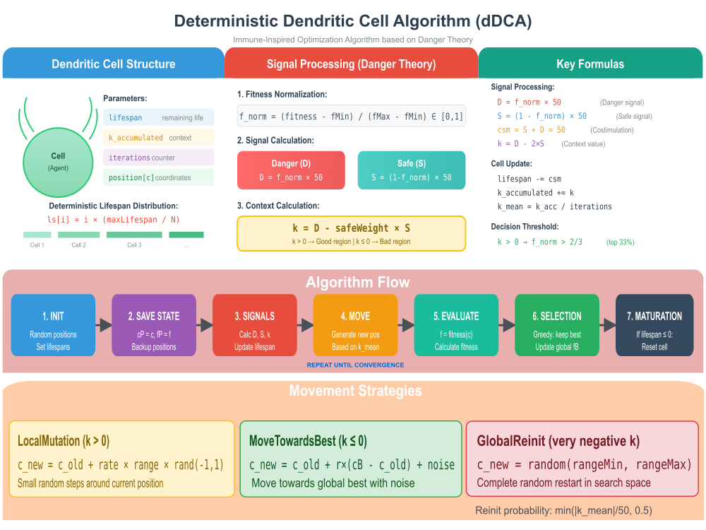
Figure 1. Illustration of the dDCA algorithm in operation

The illustration shows:

• Cell Structure — the dendritic cell structure with its parameters and a visualization of the deterministic distribution of lifespan values,
• Signal Processing — calculation of danger/safe signals and context k according to Danger Theory,
• Key Formulas — all key formulas of the algorithm,
• Algorithm Flow — a step-by-step workflow diagram,
  
• Movement Strategies — three movement strategies with formulas.

Let's move on to writing the pseudocode for the dDCA algorithm.

INITIALIZATION:
For each cell i = 1..N:
lifespan[i] = i × (maxLifespan / N) // uniform distribution
k_accumulated[i] = 0
position[i] = random position in the search space

MAIN LOOP:
For each cell i:
// Save the previous state
previous_position[i] = position[i]
previous_fitness[i] = fitness[i]

// Centralized computation of statistics
fMin = min(fitness of all cells)
fMax = max(fitness of all cells)

For each cell i:
// Normalization and signal calculation
f_norm = (fitness[i] - fMin) / (fMax - fMin)
D = f_norm × 50
S = (1 - f_norm) × 50
k = D - safeWeight × S

// Update the cell state
lifespan[i] -= 50 // csm = 50 (constant)
k_accumulated[i] += k
iterations[i]++

For each cell i:
// Mean context over the lifespan
k_mean = k_accumulated[i] / iterations[i]

// Generate a new position
IF k_mean > 0:
LocalMutation(i) // Exploitation
ELSE:
reinit_prob = min(|k_mean| / 50, 0.5)
IF random < reinit_prob:
GlobalReinit(i) // Global exploration
ELSE:
MoveTowardsBest(i) // Directed exploration

// Maturation check
IF lifespan[i] ≤ 0:
Reset the cell (lifespan, k_accumulated, iterations)

Boundary control(i)

// Greedy selection
For each cell i:
IF previous_fitness[i] > fitness[i]:
Restore the previous position and fitness

Update the global best solution

We can now start writing the code for the algorithm. The Dendritic Cell structure (S_dDCA_Cell) models a single “dendritic cell”, a system element with specific properties and a life cycle.

Main characteristics of the cell:

• lifespan — the current amount of time for which a cell can still exist or function. This indicator decreases over time.
• k_accumulated (accumulated context) — a value that reflects the information or “context” accumulated within a cell.
• initial_lifespan (initial lifespan) — the initial value of a cell's lifespan. Used to reset the cell to its initial state.
• iterations (iteration counter) — tracks how many times a cell has gone through a full processing cycle, or “incarnation,” since the last reset.

Cell methods (actions):

• Init() Initialization:

  • Sets the initial values for the cell's parameters when the cell is created.
  • lifespan and initial_lifespan are set to the value passed as “ls” (initial lifespan).
  • k_accumulated — reset to zero (starting with a clean slate).
  • iterations — set to zero, since this is the first “incarnation.”

• Reset() Reset:

• Restores the cell to its original state.
• lifespan — reset to the value of “initial_lifespan”.
• k_accumulated — reset to zero.
• iterations — also reset to zero in preparation for a new operating cycle.

//————————————————————————————————————————————————————————————————————
// Dendritic cell structure
struct S_dDCA_Cell
{
    double lifespan;          // Current lifespan
    double k_accumulated;     // Accumulated context
    double initial_lifespan;  // Initial lifespan (for reset)
    int    iterations;        // Iteration counter in the current incarnation

    void Init (double ls)
    {
      lifespan         = ls;
      initial_lifespan = ls;
      k_accumulated    = 0.0;
      iterations       = 0;
    }

    void Reset ()
    {
      lifespan      = initial_lifespan;
      k_accumulated = 0.0;
      iterations    = 0;
    }
};
//————————————————————————————————————————————————————————————————————

The C_AO_dDCA class is an implementation of the deterministic Dendritic Cell Algorithm (dDCA) for solving problems involving the search for optimal solutions. It inherits from the base class C_AO, which provides a general framework for optimization algorithms.

Public class members:

The C_AO_dDCA() constructor —

• initializes the algorithm's main attributes,
• sets the default parameters,
• creates an array called "params" to store parameters along with their names and current values.

SetParams() Parameter setup —

• a method for updating the algorithm's internal parameters based on the values stored in the "params" array,
• after setting the values, it performs boundary control to ensure they are valid, enforcing the minimum and maximum permissible values.

Init() Initialization —

• a public method for initializing the algorithm — it takes the search intervals (rangeMinP, rangeMaxP, rangeStepP) and the number of epochs (epochsP),
• calls the standard initialization procedure (StandardInit) and, if it succeeds, performs dDCA-specific initialization:
  • creates an array of "cells" with a size equal to popSize;
  • initializes each cell using the Init method, setting its initial lifespan to a uniformly distributed value between 0 and maxLifespan, which creates diversity in the cells' "age", as described in the authors' original article;
  • initializes variables to track the minimum (fMin_pop) and maximum (fMax_pop) fitness function values in the population.

Moving() Movement — a public method responsible for the main loop of the algorithm, where cells "move" or are updated in the search space.

Revision() Revision — a public method that performs corrective and evaluative actions upon completion of the Moving phase.

Public data members:

• maxLifespan (maximum lifespan) — the maximum lifespan value for cells,
• safeWeight (safe signal weight) — a parameter that affects the calculation of the cell's context,
• mutationRate (mutation rate) — a parameter that determines the magnitude of local mutations.

Private class members:

• cells [] (array of cells) — an array containing objects of type S_dDCA_Cell, representing a population of dendritic cells,
• fMin_pop (minimum fitness in the population) — stores the minimum fitness function value found among all cells in the current population,
• fMax_pop (maximum fitness in the population) — stores the maximum fitness function value found among all cells in the current population.

Private methods:

• CalculateSignals() (signal calculation) — a method for calculating various signals (e.g., Danger (D), Safe (S), ClonalSelectionMarker (csm), Context (k)) based on the normalized fitness value (f_norm);
• GenerateNewPosition() (new position generation) — a method for determining a new cell position in the search space based on the population's mean context (k_mean);
• LocalMutation() (local mutation) — applies small random changes to the cell's parameters (its "position");
• MoveTowardsBest() (movement toward the best position) — moves the cell toward the best position found so far;
• GlobalReinit() (global reinitialization) — completely reinitializes the cell;
• BoundaryControl() (boundary control) — ensures that the cell parameters remain within the valid search boundaries;
• GetNormalizedFitness() (obtaining normalized fitness) — converts the fitness function value to a normalized range, which is necessary for correct signal calculation.

//————————————————————————————————————————————————————————————————————
class C_AO_dDCA : public C_AO
{
  public:
  ~C_AO_dDCA () { }

  C_AO_dDCA ()
  {
    ao_name = "dDCA";
    ao_desc = "Deterministic Dendritic Cell Algorithm";
    ao_link = "https://www.mql5.com/en/articles/20430";

    popSize      = 50;
    maxLifespan  = 20.0;    // Maximum lifespan limit
    safeWeight   = 2.0;     // Safe signal weight: k = D - safeWeight*S
    mutationRate = 0.01;    // Local mutation strength

    ArrayResize (params, 4);
    params [0].name = "popSize";      params [0].val = popSize;
    params [1].name = "maxLifespan";  params [1].val = maxLifespan;
    params [2].name = "safeWeight";   params [2].val = safeWeight;
    params [3].name = "mutationRate"; params [3].val = mutationRate;
  }

  void SetParams ()
  {
    popSize      = (int)params [0].val;
    maxLifespan  = params      [1].val;
    safeWeight   = params      [2].val;
    mutationRate = params      [3].val;

    if (popSize < 2) popSize = 2;
    if (maxLifespan < 1.0) maxLifespan = 1.0;
    if (safeWeight < 0.0) safeWeight = 0.0;
    if (mutationRate < 0.0) mutationRate = 0.0;
    if (mutationRate > 1.0) mutationRate = 1.0;
  }

  bool Init (const double &rangeMinP  [],
             const double &rangeMaxP  [],
             const double &rangeStepP [],
             const int     epochsP);

  void Moving   ();
  void Revision ();

  //------------------------------------------------------------------
  double maxLifespan;
  double safeWeight;
  double mutationRate;

  private: //---------------------------------------------------------
  S_dDCA_Cell cells [];

  double fMin_pop;        // Minimum fitness in the population
  double fMax_pop;        // Maximum fitness in the population

  void   CalculateSignals     (double f_norm, double &D, double &S, double &csm, double &k);
  void   GenerateNewPosition  (int idx, double k_mean);
  void   LocalMutation        (int idx);
  void   MoveTowardsBest      (int idx);
  void   GlobalReinit         (int idx);
  void   BoundaryControl      (int idx);
  double GetNormalizedFitness (double f);
};
//————————————————————————————————————————————————————————————————————

The Init method of the C_AO_dDCA class is responsible for the initial setup and for preparing the algorithm to run. It receives information about the parameter search range, search steps, and the number of epochs. As the first step, the "StandardInit" method is called, which performs the general initialization required for all optimization algorithms.

The size of the "cells" array, which stores all the "dendritic cells," is set to popSize — the value that determines the number of cells in the population. lifespanIncrement is calculated — the amount by which the lifespan of each subsequent cell will increase. This is done by dividing the maximum lifespan (maxLifespan) by the total number of cells (popSize).

In the loop, the following happens for each cell: the initial lifespan for the current cell is calculated; each cell receives its own unique initial lifespan, uniformly distributed over the interval from lifespanIncrement to maxLifespan; and the Init method is called for the current cell, with the calculated "ls" value passed to it. This sets up the cell with its individual lifespan and resets the accumulated context and the iteration counter.

This division of the lifespan into different intervals allows cells to have different "observation windows" or "activity periods" during the algorithm's operation, which corresponds to one of the key ideas in the original article on dDCA.

At the end of the method, 'true' is returned, indicating that the algorithm initialization was successful.

//————————————————————————————————————————————————————————————————————
bool C_AO_dDCA::Init (const double &rangeMinP  [],
                      const double &rangeMaxP  [],
                      const double &rangeStepP [],
                      const int     epochsP)
{
  if (!StandardInit (rangeMinP, rangeMaxP, rangeStepP)) return false;

  //------------------------------------------------------------------
  // Initialization of cells with a uniform lifespan distribution
  // This provides different "time windows," as described in the authors' article
  //------------------------------------------------------------------
  ArrayResize (cells, popSize);

  double lifespanIncrement = maxLifespan / popSize;

  for (int i = 0; i < popSize; i++)
  {
    double ls = (i + 1) * lifespanIncrement;
    cells [i].Init (ls);
  }

  //------------------------------------------------------------------

  return true;
}
//————————————————————————————————————————————————————————————————————

The Moving method is the main operating loop of the dDCA algorithm. It is a sequence of steps that simulate the behavior of dendritic cells during the search for a solution.

Iteration 1. Random initialization of the population.

• If the "revision" variable is set to 'false' (indicating the first iteration), the initial positions of all cells are randomly distributed within the specified ranges (rangeMin, rangeMax).
• The u.RNDfromCI method generates a random value within the specified interval.
• The u.SeInDiSp method snaps the generated value to the specified step size (rangeStep), ensuring that the search is discrete.
• After initialization, "revision" is set to 'true', and the method completes execution, preparing for the main processing in the next iteration.

Saving the current coordinates and fitness value. This step is performed before any further calculations.

• For each cell, the current coordinates are copied to the previous coordinates, and the current fitness value is copied to the previous fitness value.
• Important: This is a critical step, as it saves the population's state at the start of the current iteration, which will be used for calculations during that iteration.

Updating population statistics for normalization:

• The variables fMin_pop (minimum fitness) and fMax_pop (maximum fitness) are initialized with extreme values;
• By iterating through all cells, the algorithm searches for the true minimum and maximum fitness function values among all cells whose value is not -DBL_MAX (the fitness has not yet been calculated);
• Protection against invalid values — if, after iterating through the population, fMax_pop remains -DBL_MAX or fMin_pop remains DBL_MAX (which can happen if all fitness values are invalid or the population is not initialized), default values are set (1.0 and 0.0, respectively) to avoid errors during subsequent normalization.

Signal processing and cell state updates. This block simulates "sensitivity" and "signal propagation" in a population of dendritic cells.

• For each cell, the normalized fitness function value is computed using the GetNormalizedFitness method, and the CalculateSignals method is called to determine the Danger (D), Safe (S), Clonal Selection Marker (csm), and Context (k) signals. These signals represent the current environment's "danger" (D), the "safe" signal (S), the clonal selection marker (csm), and the "context" (k) — the cell's internal state. Next:
  • Cell state update:
    • cells[i].lifespan -= csm: The cell's lifespan is reduced in proportion to the clonal selection marker.
    • cells[i].k_accumulated += k: The value of the "Context" signal (k) is accumulated in the cell's k_accumulated field.
    • cells[i].iterations++: The cell's iteration counter is incremented.

Generation of new positions. At this stage, decisions are made about the subsequent behavior of each cell.

For each cell:

• calculation of the mean context — the mean value of the cell's accumulated context, "k_mean", is calculated over all of its iterations;
• if a cell has "matured," a decision is made based on its accumulated context;
• If the cell has not matured, the exploration continues using the current strategy, which also depends on the accumulated context;
• In both cases (whether it has matured or not), the "GenerateNewPosition" method is called;
• After determining the new position, the "BoundaryControl" method ensures that the cell coordinates remain within the valid search boundaries (rangeMin, rangeMax).

Overall, the "Moving" method simulates:

• the first phase — random distribution of the initial points,
• state preservation — recording the best results before changes begin,
• population assessment — determining the current range of solution quality,
• signal processing — each cell "senses" its environment (represented by its fitness value) and generates internal signals (D, S, csm, k),
• lifespan management — a cell's lifespan is regulated by the "csm" signal,
• context accumulation — information about the "health" and "danger" of the environment is accumulated in "k_accumulated",
• decision-making — mature cells make more radical decisions, while young cells continue exploration,
• strategy application — a new position is generated based on the accumulated context (k_mean), allowing the cells to adapt to the local or global conditions.

//————————————————————————————————————————————————————————————————————
void C_AO_dDCA::Moving ()
{
  //------------------------------------------------------------------
  // Iteration 1: Random initialization of the population
  //------------------------------------------------------------------
  if (!revision)
  {
    for (int i = 0; i < popSize; i++)
    {
      for (int c = 0; c < coords; c++)
      {
        a [i].c [c] = u.RNDfromCI (rangeMin [c], rangeMax [c]);
        a [i].c [c] = u.SeInDiSp (a [i].c [c], rangeMin [c], rangeMax [c], rangeStep [c]);
      }
    }

    revision = true;
    return;
  }

  //------------------------------------------------------------------
  // STEP 1: Save the current coordinates and fitness
  // IMPORTANT: This must be done first, before any calculations!
  // a[i].f contains the fitness calculated after the previous Moving() call
  //------------------------------------------------------------------
  for (int i = 0; i < popSize; i++)
  {
    ArrayCopy (a [i].cP, a [i].c, 0, 0, coords);
    a [i].fP = a [i].f;
  }

  //------------------------------------------------------------------
  // STEP 2: Update the population statistics for normalization
  // Use fP (the current fitness value just saved)
  //------------------------------------------------------------------
  fMin_pop =  DBL_MAX;
  fMax_pop = -DBL_MAX;

  for (int i = 0; i < popSize; i++)
  {
    if (a [i].fP != -DBL_MAX)  // Initialization check
    {
      if (a [i].fP > fMax_pop) fMax_pop = a [i].fP;
      if (a [i].fP < fMin_pop) fMin_pop = a [i].fP;
    }
  }

  // Protection against invalid values
  if (fMax_pop == -DBL_MAX || fMin_pop == DBL_MAX)
  {
    fMax_pop = 1.0;
    fMin_pop = 0.0;
  }

  //------------------------------------------------------------------
  // STEP 3: Signal processing and cell state updates
  // Centralized processing, as in the original dDCA
  //------------------------------------------------------------------
  for (int i = 0; i < popSize; i++)
  {
    // Fitness normalization
    double f_norm = GetNormalizedFitness (a [i].fP);

    // Signal Calculation
    double D, S, csm, k;
    CalculateSignals (f_norm, D, S, csm, k);

    // Updating the Cell State
    cells [i].lifespan -= csm;
    cells [i].k_accumulated += k;
    cells [i].iterations++;
  }

  //------------------------------------------------------------------
  // STEP 4: Generating New Positions
  //------------------------------------------------------------------
  for (int i = 0; i < popSize; i++)
  {
    // Mean context over the lifespan
    double k_mean = cells [i].k_accumulated / MathMax (cells [i].iterations, 1);

    // Maturation check
    if (cells [i].lifespan <= 0.0)
    {
      // The cell has matured — we make a decision based on the accumulated context
      GenerateNewPosition (i, k_mean);
      cells [i].Reset ();
    }
    else
    {
      // The cell has not matured — we continue exploration using the current strategy
      // The strategy depends on the accumulated context
      GenerateNewPosition (i, k_mean);
    }

    BoundaryControl (i);
  }
}
//————————————————————————————————————————————————————————————————————

The GetNormalizedFitness method is responsible for scaling (normalizing) the fitness function value to the standard range from 0 to 1. This is important so that different fitness functions or fitness values obtained in different search states can be correctly compared and used in further calculations.

//————————————————————————————————————————————————————————————————————
// Normalizing fitness to the range [0, 1]
//————————————————————————————————————————————————————————————————————
double C_AO_dDCA::GetNormalizedFitness (double f)
{
  if (f == -DBL_MAX) return 0.5;

  double range = fMax_pop - fMin_pop;
  if (range < 1e-10) return 0.5;

  double norm = (f - fMin_pop) / range;

  // Clamp to [0, 1]
  if (norm < 0.0) norm = 0.0;
  if (norm > 1.0) norm = 1.0;

  return norm;
}
//————————————————————————————————————————————————————————————————————

The CalculateSignals method takes the "fitness" metric of an element that has already been converted to a universal scale. Based on this indicator, it calculates four new characteristics that reflect:

• (S) — indicates how "promising" or "attractive" this element is,
• (D) — indicates how "unpromising" or "less attractive" the element is.

"Co-stimulation" (csm). This is an overall value that takes both "danger" and "safety" into account. In this specific implementation, it will always be equal to 50 if the original fitness-based indicator was scaled to the range from 0 to 50.

"Context" (k). This is a more complex value that takes "danger" into account, while also considering the extent to which "safety" can suppress it. It helps assess how much we should actually rely on a "danger signal," given the presence of "safe" factors.

Thus, the method transforms a single input quality indicator into several new ones that describe its "attractive" and "repulsive" properties in greater detail, taking different aspects into account for decision-making.

//————————————————————————————————————————————————————————————————————
// Calculation of signals D and S
//
// Formulas from the article (normalized to [0, 50], as in the experiment):
//   csm = S + D      (1) - co-stimulation
//   k = D - 2*S      (4) - context (or D - safeWeight*S)
//
// Interpretation for optimization:
//   D  = low fitness = need to move away
//   S  = high fitness = promising region
//————————————————————————————————————————————————————————————————————
void C_AO_dDCA::CalculateSignals (double f_norm, double &D, double &S, double &csm, double &k)
{
  // Normalization to the [0, 50] range, as in the article
  D = f_norm * 50.0;
  S = (1.0 - f_norm) * 50.0;

  // Formula (1): csm = S + D = 50 (a constant under this normalization)
  csm = S + D;

  // Formula (4): k = D - safeWeight * S
  k = D - safeWeight * S;
}
//————————————————————————————————————————————————————————————————————

The GenerateNewPosition method determines how a new position (or solution) will be generated for a specific agent in the algorithm, based on the "context" of the current situation. This context is described by the mean value "k_mean".

If "k_mean" is positive, this means that the current search region is considered "good" or "promising." In this case, the method selects the exploitation strategy — that is, local mutation. The agent remains near its current position and makes small, precise adjustments, as if "refining" or "exploring" the finest details in this favorable area.

If "k_mean" is non-positive, this indicates that the current search region is considered "poor" or "less promising." Here, the algorithm switches to an exploration strategy designed to escape this zone:

Reinitialization probability. The method first generates a random number. This number is compared to the reinitialization probability (reinit_prob). This probability increases as “k_mean” becomes more negative (i.e., as the context worsens) and is capped at an upper bound (for example, 0.5, meaning no more than 50% of cases).

If the random number is less than the reinitialization probability. Global reinitialization is performed. This means that the agent is completely “reset” and placed at an entirely new, random position in the search space. It is like starting over from scratch in another part of the search space.

Otherwise (if the random number is greater than the reinitialization probability). A move toward the best solution is performed. This means that the agent attempts to move toward the best solution found so far, hoping that this will lead it to a better part of the search space while bypassing the current poor region.

Thus, the GenerateNewPosition method acts as a “smart” way to generate new solutions:

• rewards “good” regions by allowing agents to explore them in detail;
• moves agents out of “bad” regions, either by giving them a chance for a “lucky break” (global reinitialization) or by directing them toward a previously found successful solution (movement toward the best).

//————————————————————————————————————————————————————————————————————
// Generating a New Position Based on Context
//
// k > 0: good region (analogous to “mature” in dDCA)
//   ? local mutation (exploitation)
//
// k <= 0: poor region (analogous to “semi-mature” in dDCA)
//   ? movement toward the best solution or reinitialization (exploration)
//————————————————————————————————————————————————————————————————————
void C_AO_dDCA::GenerateNewPosition (int idx, double k_mean)
{
  if (k_mean > 0.0)
  {
    // Positive context — a good region
    // Local exploration around the current position
    LocalMutation (idx);
  }
  else
  {
    // Negative context — a poor region
    // Need to move away: either toward a better solution or randomly

    double r = u.RNDfromCI (0.0, 1.0);

    // The worse the context (the more negative k is), the higher the chance of reinitialization
    double reinit_prob = MathMin (MathAbs (k_mean) / 50.0, 0.5);

    if (r < reinit_prob)
    {
      // Global reinitialization
      GlobalReinit (idx);
    }
    else
    {
      // Move toward a better solution
      MoveTowardsBest (idx);
    }
  }
}
//————————————————————————————————————————————————————————————————————

The LocalMutation method introduces small, random changes to each coordinate of the element's current position. These changes occur within the defined boundaries of the search domain for each coordinate and depend on the overall "mutation rate," making it possible to explore solutions "neighboring" the current one.

//————————————————————————————————————————————————————————————————————
// Local mutation—exploration of the neighborhood of the current position
//————————————————————————————————————————————————————————————————————
void C_AO_dDCA::LocalMutation (int idx)
{
  for (int c = 0; c < coords; c++)
  {
    double range    = rangeMax [c] - rangeMin [c];
    double mutation = mutationRate * range * u.RNDfromCI (-1.0, 1.0);

    a [idx].c [c] = a [idx].cP [c] + mutation;
  }
}
//————————————————————————————————————————————————————————————————————

The MoveTowardsBest method describes a strategy in which the agent attempts to move closer to the best known solution while adding some random "noise" to preserve its exploration capabilities. The method balances exploitation (moving toward the best solution found) and exploration (sudden, small random deviations around the movement trajectory). This allows the element to move effectively toward promising regions, while avoiding getting too firmly "stuck" at a single point and maintaining the ability to find new — and perhaps even better — solutions.

//————————————————————————————————————————————————————————————————————
// Moving toward the best-known solution with noise
//————————————————————————————————————————————————————————————————————
void C_AO_dDCA::MoveTowardsBest (int idx)
{
  // Check: if cB has not yet been initialized, perform a local mutation
  if (fB == -DBL_MAX)
  {
    LocalMutation (idx);
    return;
  }

  for (int c = 0; c < coords; c++)
  {
    double r     = u.RNDfromCI (0.0, 1.0);
    double range = rangeMax [c] - rangeMin [c];

    // Move toward the best solution + random noise
    a [idx].c [c] = a [idx].cP [c]
                    + r * (cB [c] - a [idx].cP [c])
                    + mutationRate * range * u.RNDfromCI (-1.0, 1.0);
  }
}
//————————————————————————————————————————————————————————————————————

The GlobalReinit method places the element at a completely new, randomly selected point in the search space. This acts as a "complete reset" or a "leap" into an entirely different part of the solution space. This approach can be useful if the algorithm is stuck in a local optimum and needs to be "pushed" out of it in order to start exploration from scratch.

//————————————————————————————————————————————————————————————————————
// Global reinitialization—a completely random position
//————————————————————————————————————————————————————————————————————
void C_AO_dDCA::GlobalReinit (int idx)
{
  for (int c = 0; c < coords; c++)
  {
    a [idx].c [c] = u.RNDfromCI (rangeMin [c], rangeMax [c]);
  }
}
//————————————————————————————————————————————————————————————————————

This method is designed to keep an element (agent, particle) within the specified permissible boundaries for its coordinates. If an element ends up outside these boundaries, the method attempts to bring it back within them using various strategies.

The BoundaryControl method is a corrective mechanism. It ensures that the elements do not go beyond the defined search space. The "reflection" strategy allows an element to "bounce off" the boundary and return to the feasible region, while retaining some information about its movement. Additional randomization when crossing the boundary helps prevent the search from getting stuck. Finally, the last line ensures that the position conforms to the discrete rules of the space.

//————————————————————————————————————————————————————————————————————
// Boundary control with reflection
//————————————————————————————————————————————————————————————————————
void C_AO_dDCA::BoundaryControl (int idx)
{
  for (int c = 0; c < coords; c++)
  {
    if (a [idx].c [c] < rangeMin [c])
    {
      a [idx].c [c] = rangeMin [c] + MathAbs (a [idx].c [c] - rangeMin [c]);

      if (a [idx].c [c] > rangeMax [c])
      {
        a [idx].c [c] = u.RNDfromCI (rangeMin [c], rangeMax [c]);
      }
    }

    if (a [idx].c [c] > rangeMax [c])
    {
      a [idx].c [c] = rangeMax [c] - MathAbs (a [idx].c [c] - rangeMax [c]);

      if (a [idx].c [c] < rangeMin [c])
      {
        a [idx].c [c] = u.RNDfromCI (rangeMin [c], rangeMax [c]);
      }
    }

    a [idx].c [c] = u.SeInDiSp (a [idx].c [c], rangeMin [c], rangeMax [c], rangeStep [c]);
  }
}
//————————————————————————————————————————————————————————————————————

The Revision method performs two key functions:

1. selection — it determines whether to keep the agent's new (potentially improved) position or return to the previous best one,
2. updating the global best — it tracks the globally best position found among all agents and stores this information.

Selection: greedy selection. The essence of selection. This block implements a greedy strategy. If the agent's new position turns out to be worse than its own best known position, the agent will "never forget" its previous best position and will return to it.

The Revision method is used to stabilize and track the population's progress. It ensures that each agent does not lose its best found solutions through greedy selection and helps identify the overall best solution found across the entire population. Since the algorithm is designed for maximization problems, fB and cB will store the best results.

//————————————————————————————————————————————————————————————————————
void C_AO_dDCA::Revision ()
{
  //------------------------------------------------------------------
  // Selection: greedy selection — keep the position if it is better
  //------------------------------------------------------------------
  for (int i = 0; i < popSize; i++)
  {
    // If the previous fitness is better than the current fitness, revert
    if (a [i].fP > a [i].f && a [i].fP != -DBL_MAX)
    {
      a [i].f = a [i].fP;
      ArrayCopy (a [i].c, a [i].cP, 0, 0, coords);
    }
  }

  //------------------------------------------------------------------
  // Update the global best 
  //------------------------------------------------------------------
  for (int i = 0; i < popSize; i++)
  {
    if (a [i].f > fB)
    {
      fB = a [i].f;
      ArrayCopy (cB, a [i].c, 0, 0, coords);
    }
  }
}
//————————————————————————————————————————————————————————————————————

Test Results

Now we can look at the results of testing the algorithm on our test functions: the algorithm achieves 41% and performs worst on discrete functions.

dDCA|Deterministic Dendritic Cell Algorithm|50.0|20.0|2.0|0.01|
=============================
5 Hilly's; Func runs: 10000; result: 0.8798800651743539
25 Hilly's; Func runs: 10000; result: 0.4788852312258377
500 Hilly's; Func runs: 10000; result: 0.27717376068435823
=============================
5 Forest's; Func runs: 10000; result: 0.6340906667281795
25 Forest's; Func runs: 10000; result: 0.3689169839474446
500 Forest's; Func runs: 10000; result: 0.21510602459276465
=============================
5 Megacity's; Func runs: 10000; result: 0.5292307692307692
25 Megacity's; Func runs: 10000; result: 0.2163076923076923
500 Megacity's; Func runs: 10000; result: 0.10510769230769328
=============================
All score: 3.70470 (41.16%)

The visualization shows a wide spread of results on low-dimensional functions and low convergence metrics on the discrete Megacity function. The population is divided into groups of agent cells that explore promising regions, but this is not sufficient for an overall search of the entire solution space.

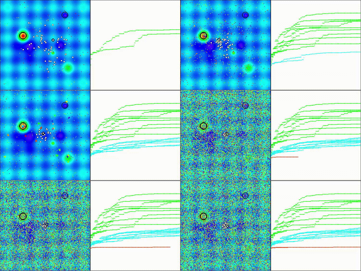
dDCA on the Hilly test function

dDCA on the Forest test function

dDCA on the Megacity test function

To get a general idea of how the dDCA algorithm works, let us examine its behavior on standard test functions that are not used in our testing but have their own specific purposes. The variation in values is less noticeable.

dDCA on the standard Ackley test function

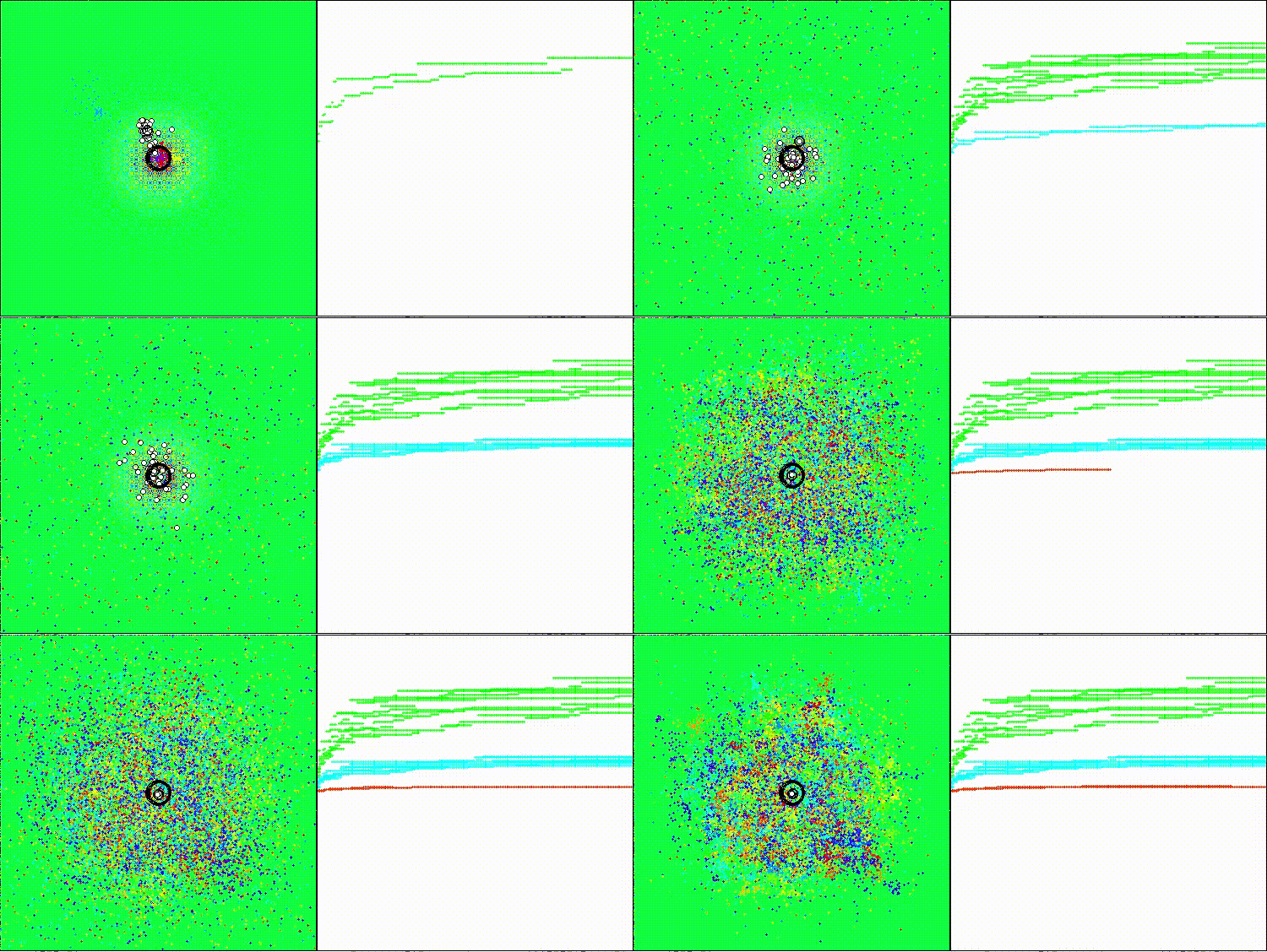
dDCA on the standard Shaffer test function

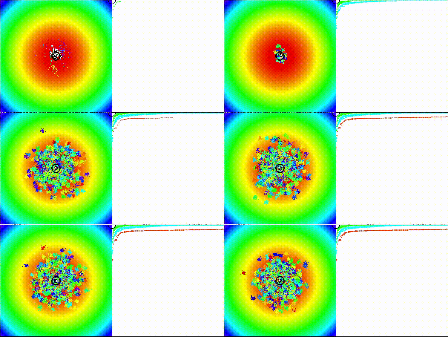
dDCA on the standard Paraboloid test function

The dDCA algorithm is included in our ranking table of the best population-based optimization methods for reference.

No.	AO	Description	Hilly			Hilly Final	Forest			Forest Final	Megacity (discrete)			Megacity Final	Final Result	% of MAX
			10 p (5 F)	50 p (25 F)	1,000 p (500 F)		10 p (5 F)	50 p (25 F)	1,000 p (500 F)		10 p (5 F)	50 p (25 F)	1,000 p (500 F)
1	DOAdingom	dingo_optimization_algorithm_M	0.47968	0.45367	0.46369	1.39704	0.94145	0.87909	0.91454	2.73508	0.78615	0.86061	0.84805	2.49481	6.627	73.63
2	ANS	across neighbourhood search	0.94948	0.84776	0.43857	2.23581	1.00000	0.92334	0.39988	2.32323	0.70923	0.63477	0.23091	1.57491	6.134	68.15
3	CLA	code lock algorithm (joo)	0.95345	0.87107	0.37590	2.20042	0.98942	0.91709	0.31642	2.22294	0.79692	0.69385	0.19303	1.68380	6.107	67.86
4	AMOm	animal migration optimization M	0.90358	0.84317	0.46284	2.20959	0.99001	0.92436	0.46598	2.38034	0.56769	0.59132	0.23773	1.39675	5.987	66.52
5	(P+O)ES	(P+O) evolution strategies	0.92256	0.88101	0.40021	2.20379	0.97750	0.87490	0.31945	2.17185	0.67385	0.62985	0.18634	1.49003	5.866	65.17
6	CTA	comet tail algorithm (joo)	0.95346	0.86319	0.27770	2.09435	0.99794	0.85740	0.33949	2.19484	0.88769	0.56431	0.10512	1.55712	5.846	64.96
7	TETA	time evolution travel algorithm (joo)	0.91362	0.82349	0.31990	2.05701	0.97096	0.89532	0.29324	2.15952	0.73462	0.68569	0.16021	1.58052	5.797	64.41
8	SDSm	stochastic diffusion search M	0.93066	0.85445	0.39476	2.17988	0.99983	0.89244	0.19619	2.08846	0.72333	0.61100	0.10670	1.44103	5.709	63.44
9	BOAm	billiards optimization algorithm M	0.95757	0.82599	0.25235	2.03590	1.00000	0.90036	0.30502	2.20538	0.73538	0.52523	0.09563	1.35625	5.598	62.19
10	AAm	archery algorithm M	0.91744	0.70876	0.42160	2.04780	0.92527	0.75802	0.35328	2.03657	0.67385	0.55200	0.23738	1.46323	5.548	61.64
11	ESG	evolution of social groups (joo)	0.99906	0.79654	0.35056	2.14616	1.00000	0.82863	0.13102	1.95965	0.82333	0.55300	0.04725	1.42358	5.529	61.44
12	SIA	simulated isotropic annealing (joo)	0.95784	0.84264	0.41465	2.21513	0.98239	0.79586	0.20507	1.98332	0.68667	0.49300	0.09053	1.27020	5.469	60.76
13	EOm	extremal_optimization_M	0.76166	0.77242	0.31747	1.85155	0.99999	0.76751	0.23527	2.00277	0.74769	0.53969	0.14249	1.42987	5.284	58.71
14	BBO	biogeography-based optimization	0.94912	0.69456	0.35031	1.99399	0.93820	0.67365	0.25682	1.86867	0.74615	0.48277	0.17369	1.40261	5.265	58.50
15	ACS	artificial cooperative search	0.75547	0.74744	0.30407	1.80698	1.00000	0.88861	0.22413	2.11274	0.69077	0.48185	0.13322	1.30583	5.226	58.06
16	DA	dialectical algorithm	0.86183	0.70033	0.33724	1.89940	0.98163	0.72772	0.28718	1.99653	0.70308	0.45292	0.16367	1.31967	5.216	57.95
17	BHAm	black hole algorithm M	0.75236	0.76675	0.34583	1.86493	0.93593	0.80152	0.27177	2.00923	0.65077	0.51646	0.15472	1.32195	5.196	57.73
18	ASO	anarchy society optimization	0.84872	0.74646	0.31465	1.90983	0.96148	0.79150	0.23803	1.99101	0.57077	0.54062	0.16614	1.27752	5.178	57.54
19	RFO	royal flush optimization (JOO)	0.83361	0.73742	0.34629	1.91733	0.89424	0.73824	0.24098	1.87346	0.63154	0.50292	0.16421	1.29867	5.089	56.55
20	AOSm	atomic orbital search M	0.80232	0.70449	0.31021	1.81702	0.85660	0.69451	0.21996	1.77107	0.74615	0.52862	0.14358	1.41835	5.006	55.63
21	TSEA	turtle shell evolution algorithm (JOO)	0.96798	0.64480	0.29672	1.90949	0.99449	0.61981	0.22708	1.84139	0.69077	0.42646	0.13598	1.25322	5.004	55.60
22	BSA	backtracking_search_algorithm	0.97309	0.54534	0.29098	1.80941	0.99999	0.58543	0.21747	1.80289	0.84769	0.36953	0.12978	1.34700	4.959	55.10
23	DE	differential evolution	0.95044	0.61674	0.30308	1.87026	0.95317	0.78896	0.16652	1.90865	0.78667	0.36033	0.02953	1.17653	4.955	55.06
24	SRA	successful restaurateur algorithm (JOO)	0.96883	0.63455	0.29217	1.89555	0.94637	0.55506	0.19124	1.69267	0.74923	0.44031	0.12526	1.31480	4.903	54.48
25	BO	bonobo_optimizer	0.77565	0.63805	0.32908	1.74278	0.88088	0.76344	0.25573	1.90005	0.61077	0.49846	0.14246	1.25169	4.895	54.38
26	CRO	chemical reaction optimization	0.94629	0.66112	0.29853	1.90593	0.87906	0.58422	0.21146	1.67473	0.75846	0.42646	0.12686	1.31178	4.892	54.36
27	BIO	blood inheritance optimization (JOO)	0.81568	0.65336	0.30877	1.77781	0.89937	0.65319	0.21760	1.77016	0.67846	0.47631	0.13902	1.29378	4.842	53.80
28	DOA	dream_optimization_algorithm	0.85556	0.70085	0.37280	1.92921	0.73421	0.48905	0.24147	1.46473	0.77231	0.47354	0.18561	1.43146	4.825	53.62
29	BSA	bird swarm algorithm	0.89306	0.64900	0.26250	1.80455	0.92420	0.71121	0.24939	1.88479	0.69385	0.32615	0.10012	1.12012	4.809	53.44
30	DEA	dolphin_echolocation_algorithm	0.75995	0.67572	0.34171	1.77738	0.89582	0.64223	0.23941	1.77746	0.61538	0.44031	0.15115	1.20684	4.762	52.91
31	HS	harmony search	0.86509	0.68782	0.32527	1.87818	0.99999	0.68002	0.09590	1.77592	0.62000	0.42267	0.05458	1.09725	4.751	52.79
32	SSG	saplings sowing and growing	0.77839	0.64925	0.39543	1.82308	0.85973	0.62467	0.17429	1.65869	0.64667	0.44133	0.10598	1.19398	4.676	51.95
33	BCOm	bacterial chemotaxis optimization M	0.75953	0.62268	0.31483	1.69704	0.89378	0.61339	0.22542	1.73259	0.65385	0.42092	0.14435	1.21912	4.649	51.65
34	ABO	african buffalo optimization	0.83337	0.62247	0.29964	1.75548	0.92170	0.58618	0.19723	1.70511	0.61000	0.43154	0.13225	1.17378	4.634	51.49
35	(PO)ES	(PO) evolution strategies	0.79025	0.62647	0.42935	1.84606	0.87616	0.60943	0.19591	1.68151	0.59000	0.37933	0.11322	1.08255	4.610	51.22
36	FBA	fractal-based algorithm	0.79000	0.65134	0.28965	1.73099	0.87158	0.56823	0.18877	1.62858	0.61077	0.46062	0.12398	1.19537	4.555	50.61
37	TSm	tabu search M	0.87795	0.61431	0.29104	1.78330	0.92885	0.51844	0.19054	1.63783	0.61077	0.38215	0.12157	1.11449	4.536	50.40
38	BSO	brain storm optimization	0.93736	0.57616	0.29688	1.81041	0.93131	0.55866	0.23537	1.72534	0.55231	0.29077	0.11914	0.96222	4.498	49.98
39	WOAm	whale optimization algorithm M	0.84521	0.56298	0.26263	1.67081	0.93100	0.52278	0.16365	1.61743	0.66308	0.41138	0.11357	1.18803	4.476	49.74
40	AEFA	artificial electric field algorithm	0.87700	0.61753	0.25235	1.74688	0.92729	0.72698	0.18064	1.83490	0.66615	0.11631	0.09508	0.87754	4.459	49.55
41	AEO	artificial ecosystem-based optimization algorithm	0.91380	0.46713	0.26470	1.64563	0.90223	0.43705	0.21400	1.55327	0.66154	0.30800	0.28563	1.25517	4.454	49.49
42	CAm	camel algorithm M	0.78684	0.56042	0.35133	1.69859	0.82772	0.56041	0.24336	1.63149	0.64846	0.33092	0.13418	1.11356	4.444	49.37
43	ACOm	ant colony optimization M	0.88190	0.66127	0.30377	1.84693	0.85873	0.58680	0.15051	1.59604	0.59667	0.37333	0.02472	0.99472	4.438	49.31
44	CMAES	covariance_matrix_adaptation_evolution_strategy	0.76258	0.72089	0.00000	1.48347	0.82056	0.79616	0.00000	1.61672	0.75846	0.49077	0.00000	1.24923	4.349	48.33
45	DA_duelist	duelist_algorithm	0.92782	0.53778	0.27792	1.74352	0.86957	0.47536	0.18193	1.52686	0.62153	0.33569	0.11715	1.07437	4.345	48.28
	dDCA	deterministic_dendritic_cell_algorithm	0.87988	0.47888	0.27717	1.63593	0.63409	0.36891	0.21510	1.21810	0.52923	0.21630	0.10510	0.85063	3.705	41.16
	RW	random walk	0.48754	0.32159	0.25781	1.06694	0.37554	0.21944	0.15877	0.75375	0.27969	0.14917	0.09847	0.52734	2.348	26.09

Conclusions

The proposed adaptation of the deterministic Dendritic Cell Algorithm (dDCA) for continuous optimization problems demonstrated the viability of the approach, but did not match the performance of the best population-based methods. During testing on a standard set of functions, the algorithm scored 41%, which is below the 48% threshold required for inclusion in the ranking table.

An analysis of the results revealed a distinctive feature: the algorithm performs worst on discrete functions. This is explained by the nature of the signal mechanism: smooth fitness normalization poorly reflects abrupt transitions in discrete landscapes, where neighboring solutions may be of radically different quality.

Despite the overall result, several components of the algorithm are of interest in their own right:

• deterministic lifespan distribution ensures uniform asynchrony within the population without introducing additional stochasticity;
• the context accumulation mechanism enables decisions based on statistics from multiple iterations, which improves robustness to noise in the fitness function;
• adaptive balance between exploration and exploitation based on the collective context of the population can serve as an alternative to classical schemes with an explicit parameter.

These components can be used as building blocks for hybrid algorithms or adapted for specialized tasks where robustness to noisy estimates of solution quality is important.

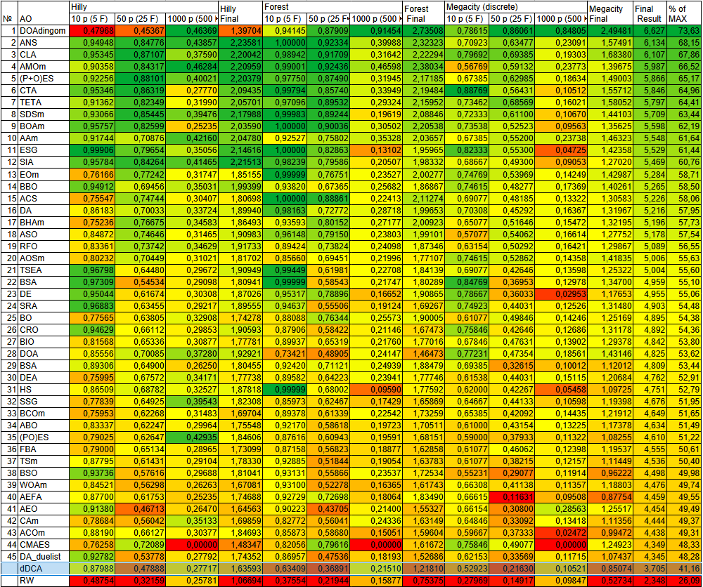
Figure 2. Color coding of algorithms for the corresponding tests

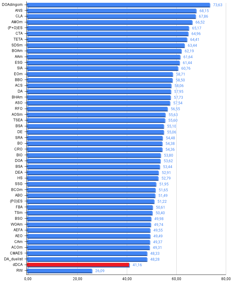
Figure 3. Histogram of algorithm testing results (on a scale from 0 to 100; the higher the score, the better, where 100 is the maximum possible theoretical result; the archive contains a script for calculating the ranking table)

Pros and cons of the dDCA algorithm:

Pros:

1. Fast.

Cons:

1. Weaker results on discrete functions.

An archive containing the latest versions of the source code for the algorithms is attached to the article. The author of this article assumes no responsibility for absolute accuracy in describing the canonical algorithms; many of them have been modified to improve their search capabilities. The conclusions and judgments presented in the articles are based on the results of the experiments performed.

• GitHub: https://github.com/JQSakaJoo/Population-optimization-algorithms-MQL5

Programs Used in the Article

#	Name	Type	Description
1	#C_AO.mqh	Include file	Parent class for population-based optimization algorithms
2	#C_AO_enum.mqh	Include file	Enumeration of population-based optimization algorithms
3	TestFunctions.mqh	Include file	Library of test functions
4	TestStandFunctions.mqh	Include file	Test bench function library
5	Utilities.mqh	Include file	Utility function library
6	CalculationTestResults.mqh	Include file	Script for calculating results for the comparison table
7	Testing AOs.mq5	Script	A unified test bench for all population-based optimization algorithms
8	Simple use of population optimization algorithms.mq5	Script	A simple example of using population-based optimization algorithms without visualization
9	Test_AO_dDCA.mq5	Script	Test bench for dDCA