

Dandelion Optimizer (DO)
 1 258
1 258
 2
2

Contents
Introduction
In this article, we examine the Dandelion Optimizer (DO), a metaheuristic algorithm inspired by the life cycle of dandelion seeds. The authors Shijie Zhao, Tianran Zhang, Shilin Ma, and Miao Chen introduced it in 2022 in the journal Engineering Applications of Artificial Intelligence.
The dandelion is one of the most common plants on the planet. The secret to its evolutionary success lies in its unique seed-dispersal mechanism. Each seed is equipped with a fluffy “parachute” (pappus) that allows it to travel significant distances through the air. The wind lifts the seeds, carries them above the ground, and then they settle in new places where they can sprout.
Implementation of the Algorithm
We have all seen how the wind picks up fluffy dandelion seeds and scatters them far and wide. This simple natural process turned out to be an interesting search strategy that researchers transformed into an optimization algorithm.
Imagine a clearing where a dandelion is growing. Its goal is to find the best places for its seeds to sprout. Seeds cannot choose their own direction, but wind, air turbulence, and the unique shape of the fluffy parachute (pappus) create complex flight paths. As a result, the seeds are spread over a wide area, and some of them find ideal conditions for growth.
The DO algorithm simulates this process. Each “seed” is a potential solution to an optimization problem. The coordinates of a seed in space are the values of the parameters to be optimized. “Soil quality” at the landing point is the value of the objective function.
Three phases of seed flight. The flight of a dandelion seed is divided into three consecutive phases, each of which plays a role in finding the optimal solution.
Phase 1: Rising stage. When the wind detaches a seed from the dandelion head, it begins to rise. Depending on the strength of the wind, two scenarios are possible. Strong wind (80% of cases) creates vortical flows, and the seed moves along a spiral trajectory, changing direction unpredictably. In the algorithm, this is implemented using a combination of trigonometric functions and the lognormal distribution:
new position = current position + α × vortex × random direction
Let's say we are optimizing two parameters of a trading strategy: the moving average period (from 10 to 200) and the stop-loss multiplier (from 1.0 to 5.0). The seed is located at the point [50, 2.0]. Vortex Rising can move it to the point [73, 2.8] — a significant jump into a new area of the search space.
Weak wind (20% of cases) lifts the seed more smoothly. It moves linearly, shifting slightly relative to its current position:
new position = center of the region + (current position - center of the region) × k
Example: the same seed [50, 2.0], with the center of the region at [105, 3.0] and k = 0.9, will move to [55.5, 2.1] — a small displacement toward the center. Why is this phase necessary? The Rising stage provides exploration of the search space. The seeds scatter in different directions, covering a large area. This helps identify promising areas that may contain the global optimum.
Phase 2: Decline. After Rising, the seed enters horizontal air currents and begins to drift. In this phase, the seeds “communicate” with one another through the mean position of the population. First, the center of mass of all the seeds is calculated:
mean = sum of all positions / number of seeds
Each seed then adjusts its trajectory based on this mean:
new position = current position - β × α × (mean - β × α × current position)
Example: suppose there are 5 seeds in the population with positions [30, 1.5], [80, 2.5], [120, 3.0], [60, 2.0], [90, 2.8]. Mean position: [76, 2.36]. The seed at position [30, 1.5] will be pulled toward this center, shifting to approximately [45, 1.8]. Why is this necessary? The Decline stage provides information exchange between seeds. If most of the seeds are concentrated in a particular area, then that area shows promise. Lagging seeds are pulled toward the group without losing their individuality.
Phase 3: Landing. Near the ground, air currents become turbulent. The seed performs a final maneuver, seeking to land in the most favorable spot — near the best solution found (the elite). To model turbulence, a Lévy flight is used — a special type of random motion with rare long jumps:
Lévy step = u / |v|^(2/3), where u and v are random numbers
new position = elite + Lévy step × α × (elite - current position × ratio)
Example: The best solution found (the elite) is at the point [85, 2.4]. A seed starting from position [60, 2.0] with a Lévy step of 0.3 and ratio = 1.0 will land approximately at [77, 2.28] — closer to the elite, but not exactly at its coordinates. The Landing stage provides exploitation of the found solutions. The seeds concentrate around the best point, carefully exploring its neighborhood. At the same time, Lévy flight preserves the possibility of a random jump — what if there is an even better solution nearby?
Adaptive parameters. A key feature of the algorithm is that its parameters automatically change during the optimization process. The “α” parameter (intensity) decreases from 1 to 0:
α = random number × (t²/T² - 2t/T + 1)
At the beginning of the optimization (t is small), “α” is close to 1, and the steps are large — the seeds actively explore the search space. Toward the end (when t is close to T), “α” approaches 0; the steps are small, and fine-tuning of the solution takes place.
An analogy: looking for lost keys. First, you quickly walk through the entire apartment (taking big steps), and when you remember that your keys are somewhere in the kitchen, you start searching every corner thoroughly (taking small steps).
The ratio parameter (progress) increases from 0 to 2: ratio = 2 × t / T. The higher the “ratio,” the more strongly the seeds are drawn toward the elite during the Landing stage. At the beginning of the search, the seeds land relatively freely; by the end, nearly all of them move toward the best solution.
Boundary control. What should you do if a seed has “flown” outside the feasible region? The algorithm uses a reflection mechanism similar to the way a ball bounces off a wall.
If position < minimum: position = minimum + (minimum - position); if position > maximum: position = maximum - (position - maximum)
Example: valid range [10, 200]. The seed tried to fly to position 220. After reflection: 200 - (220 - 200) = 180. The seed “bounced” off the boundary and ended up inside the feasible region.
If, after several reflections, the seed is still outside the bounds (for example, if it has flown very far away), it is assigned a random position within the feasible region.
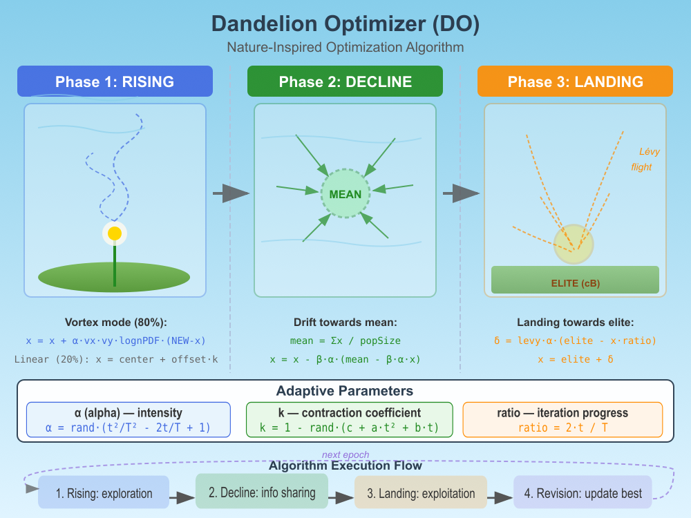
Figure 1. Illustration of the DO algorithm in operation
The illustration shows the three phases of the algorithm:
- Rising (blue) — seeds rise from the dandelion along spiral trajectories, with vortex Rising visualized using formulas.
- Decline (green) — seeds drift toward the population mean position (MEAN); the arrows indicate the direction of movement.
- Landing (orange) — seeds land near the elite position (ELITE/cB) along Lévy flight trajectories.
Additional elements: adaptive parameters "α", "k", and "ratio" with their formulas; the algorithm execution order with a loop back to the next epoch; dandelion seeds with pappus (a fluffy parachute); and the elite seed highlighted in gold. We can now start writing the code for the DO algorithm.
INITIALIZATION
1. For each seed i from 1 to popSize:
1.1. For each coordinate c:
— Assign a random value within the range [rangeMin[c], rangeMax[c]]
1.2. Calculate the seed's fitness
2. Find the best seed in the population
3. Store its coordinates in cB[] and its fitness in fB
MAIN OPTIMIZATION LOOP
4. For each epoch t from 1 to epochs:
4.1. COMPUTING ADAPTIVE PARAMETERS
— Calculate the intensity parameter alpha:
alpha decreases from 1 to 0 as t increases
(large steps at the beginning, small steps at the end)
— Calculate the compression coefficient k:
k determines the degree of compression toward the center of the region
4.2. RISING STAGE (Rising Stage)
Generate a random number rand
IF rand < 0.8 THEN
Vortex Rising (strong wind)
For each seed i:
— Compute a random angle theta in the range [-π, π]
— Compute the vortex components vx and vy
based on a logarithmic spiral
For each coordinate c:
— Generate a random point NEW in the search space
— Displace the seed toward NEW, taking into account
the vortex coefficient and the lognormal distribution
— Check and adjust the bounds
ELSE
Linear Rising (weak wind)
For each seed i:
For each coordinate c:
— Calculate the seed’s displacement relative to the center of the region
— Multiply the displacement by the coefficient k
— New position = center + scaled displacement
— Check and adjust the bounds
4.3. DECLINE STAGE (Decline Stage)
Calculating the mean position of the population
For each coordinate c:
mean[c] = sum of all x[i][c] / popSize
Seed drift toward the mean
For each seed i:
For each coordinate c:
— Generate a random beta coefficient (normal distribution)
— Calculate the displacement based on the difference between
the current position and the mean position
— Limit the displacement to 30% of the range width
— Apply the displacement to the seed position
— Check and adjust the bounds
4.4. LANDING STAGE (Landing Stage)
Calculate ratio = 2 * t / epochs
(ratio increases from 0 to 2 as the end approaches)
For each seed i:
Generating a Lévy step
For each coordinate c:
— Generate two normally distributed numbers u and v
— levy[c] = u / |v|^(2/3)
Landing toward the elite solution
For each coordinate c:
— Compute the displacement delta based on:
• the Lévy step
• the alpha parameter
• the difference between the elite position and the current position
— Limit delta to 50% of the range width
— New position = elite[c] + delta
— Check and adjust the bounds
4.5. COMPUTING FITNESS AND UPDATING THE BEST SOLUTION
For each seed i:
— Calculate the fitness of the new position
Find the seed with the best fitness in the current population
IF the best fitness in the population > fB THEN
— Update fB
— Copy the coordinates of the best seed to cB[]
COMPLETION
5. Return the best solution cB[] and its fitness fB
END OF ALGORITHM
HELPER PROCEDURE: Boundary control
PROCEDURE BoundaryControl(seed position):
For each coordinate c:
WHILE position is out of bounds AND attempts < 10:
IF position < minimum THEN
— Reflect at the lower bound:
position = minimum + (minimum - position)
IF position > maximum THEN
— Reflect at the upper bound:
position = maximum - (position - maximum)
IF the position is still out of bounds THEN
— Assign a random value within the valid bounds
— Round the position to the nearest valid step
END PROCEDURE
Now let's move on to implementing this in code. A simple structure is used to store auxiliary coordinate data:
//————————————————————————————————————————————————————————————————————
struct S_DO_Coord
{
    double v;
};
//————————————————————————————————————————————————————————————————————
The C_AO_DO class inherits from the base class "C_AO" and implements the DO algorithm.
Functionality and methods:
- SetParams — updates the algorithm's internal parameters based on the values passed via the "params" array,
- Init — initializes the algorithm based on the specified minimum and maximum search bounds for each dimension, the step size, and the number of epochs,
- Moving — is responsible for the population's movement (evolution) during the optimization process,
- Revision — used to review or adjust the positions of individuals after a certain stage,
- LevyFlight — a private method responsible for generating random steps according to the Lévy distribution, as described earlier,
- LognormalPDF — a private method for calculating the probability density value of the lognormal distribution,
- BoundaryControl — a private method used to ensure that the generated positions remain within the specified search bounds.
Internal variables:
- epochs — the maximum number of iterations (epochs),
- currentEpoch — the current iteration (epoch),
- sigma_u — a precomputed standard deviation value for the Lévy distribution at β = 1.5,
- mean — an array of the mean positions of individuals in the search space,
- levy — an array that stores the generated Lévy steps for each coordinate, used to move the individuals,
- center — an array of the center points of the search range for each coordinate,
- range — an array containing the width of the search range for each coordinate.
The C_AO_DO class encapsulates the logic of the Dandelion Optimizer algorithm, including the generation of random displacements sampled from the Lévy distribution and the management of search parameters.
//————————————————————————————————————————————————————————————————————
class C_AO_DO : public C_AO
{
  public:
  ~C_AO_DO () { }

  C_AO_DO ()
  {
    ao_name = "DO";
    ao_desc = "Dandelion Optimizer";
    ao_link = "https://www.mql5.com/ru/articles/20540";

    popSize = 50;

    ArrayResize (params, 1);
    params [0].name = "popSize"; params [0].val = popSize;
  }

  void SetParams ()
  {
    popSize = (int)params [0].val;
  }

  bool Init (const double &rangeMinP  [],
             const double &rangeMaxP  [],
             const double &rangeStepP [],
             const int     epochsP);

  void Moving   ();
  void Revision ();

  private: //—————————————————————————————————————————————————————————
  int    epochs;       // maximum iterations
  int    currentEpoch; // current iteration
  double sigma_u;      // precomputed Lévy sigma for beta = 1.5

  S_DO_Coord mean   [];  // mean position
  S_DO_Coord levy   [];  // Lévy flight steps
  S_DO_Coord center [];  // center of the search range
  S_DO_Coord range  [];  // range width

  void   LevyFlight      ();
  double LognormalPDF    (double x, double mu, double sigma);
  void   BoundaryControl (int idx);
};
//————————————————————————————————————————————————————————————————————
The Init method of the "C_AO_DO" class is responsible for the initial setup and preparation of the algorithm for operation. First, it calls the parent method StandardInit, which performs initialization procedures common to all optimizers, such as setting search ranges (minimum and maximum values, and steps) and determining the number of coordinates in the objective function. If this standard initialization fails, the Init method will also return 'false'.
Setting optimization parameters:- epochs — specifies the maximum number of iterations (epochs) that the algorithm will perform,
- currentEpoch — resets the current epoch counter to zero, since the optimization process is just beginning.
- mean — for storing mean positions,
- levy — for storing steps calculated using the Lévy distribution,
- center — for storing the centers of search regions,
- range — for storing the widths of search regions.
- center — the coordinate of the center of the search region, defined as the mean of the minimum and maximum valid values for that coordinate,
- range — the width of the search region, equal to the difference between the maximum and minimum valid values.
Sets the predefined value of "sigma_u," which is a constant used to calculate the Lévy steps when the beta parameter is set to 1.5.
The value σ u = 0.6966 (sigma_u = 0.6966) was precomputed using the formula: σ_u = (Γ(1+β) * sin(πβ/2) / (Γ((1+β)/2) * β * 2^((β-1)/2)))^(1/β); for β = 1.5, this yields a constant of ≈ 0.6966. This is done to simplify the calculations in the algorithm.
If all initialization steps are successful, the method returns 'true'. Thus, Init prepares all the necessary data structures, sets the global optimization parameters, and performs the preliminary calculations required for the proper execution of the subsequent Moving and Revision algorithm steps.
//————————————————————————————————————————————————————————————————————
bool C_AO_DO::Init (const double &rangeMinP  [],
                    const double &rangeMaxP  [],
                    const double &rangeStepP [],
                    const int     epochsP)
{
  if (!StandardInit (rangeMinP, rangeMaxP, rangeStepP)) return false;

  //------------------------------------------------------------------
  epochs       = epochsP;
  currentEpoch = 0;

  ArrayResize (mean,   coords);
  ArrayResize (levy,   coords);
  ArrayResize (center, coords);
  ArrayResize (range,  coords);

  // Precompute the center and width of the range for each coordinate
  for (int c = 0; c < coords; c++)
  {
    center [c].v = (rangeMax [c] + rangeMin [c]) * 0.5;
    range  [c].v =  rangeMax [c] - rangeMin [c];
  }

  // Precompute sigma_u for Lévy flight with beta = 1.5
  sigma_u = 0.6966;

  return true;
}
//————————————————————————————————————————————————————————————————————
The Moving method is the main working loop of the DO algorithm and is responsible for moving the population of solutions through the search space during each optimization epoch. It is divided into three main phases: the "Rising stage," the "Decline stage," and the "Landing stage," each of which uses its own specific strategy for updating positions.
If the "revision" flag is set to 'false' (i.e., this is the first iteration), the method randomly initializes the positions of all popSize individuals within the specified ranges rangeMin and rangeMax for each coordinate. The SeInDiSp function is used to correct positions taking into account the rangeStep step size. The "revision" flag is set to 'true', and the method completes execution for this first epoch.
Calculation of time parameters. The currentEpoch counter is incremented. The relative times "t" (current epoch) and "T" (maximum number of epochs) are calculated. The "alpha" parameter is calculated; it is a random number that depends on the current and maximum epochs and controls the degree of change during the Rising stage. The parameters "aa," "bb," "cc," and "k" are calculated; they are used during the linear Rising stage and control the scaling of the displacement relative to the center of the range.
Rising stage, simulating the spiral motion of a seed in an upward air current. With a probability of 0.8, vortex Rising: for each individual, random values for "theta," "row," "vx," "vy," and "vxvy" are generated to simulate vortex motion. For each coordinate of each individual:
- a random variable "lamb" is generated from a Gaussian distribution,
- the value of the lognormal distribution is calculated,
- a new random value is generated within the absolute bounds,
- the new position of the individual is calculated as the current position plus a displacement that depends on "alpha," "vxvy," "lognPDF," and the difference between "NEW" and the current position.
With a probability of 0.2, linear Rising: for each individual and each coordinate, the displacement of the current position relative to the center of the range is calculated. The new position is calculated by scaling this displacement using the "k" parameter and then returning it to the center of the range. After positions are updated in any of the Rising subphases, BoundaryControl is applied to each individual to ensure that its position remains within the valid bounds.
Decline stage: during this stage, the seeds drift in a horizontal air current. The mean position of all individuals is calculated for each coordinate. For each individual and each coordinate:
- A random "beta" parameter is generated from a Gaussian distribution,
- the "betaAlpha" parameter is calculated,
- the "delta" displacement is calculated based on "betaAlpha", the mean position, and the individual's current position,
- to prevent excessively large steps, "delta" is limited to 30% of the range width,
- the individual's position is updated by adding "delta".
- the values of the best-found position (elite, stored in cB) and the individual's current position (current) are obtained,
- the "delta" displacement is calculated using a formula that includes the Lévy step, "alpha", "elite", "current", and "ratio",
- the "delta" displacement is limited to half the width of the range,
- the individual's new position is calculated as "elite" plus "delta".
//————————————————————————————————————————————————————————————————————
void C_AO_DO::Moving ()
{
  //------------------------------------------------------------------
  // First iteration: population initialization
  if (!revision)
  {
    for (int i = 0; i < popSize; i++)
    {
      for (int c = 0; c < coords; c++)
      {
        a [i].c [c] = u.RNDfromCI (rangeMin [c], rangeMax [c]);
        a [i].c [c] = u.SeInDiSp (a [i].c [c], rangeMin [c], rangeMax [c], rangeStep [c]);
      }
    }

    revision = true;
    return;
  }

  //------------------------------------------------------------------
  currentEpoch++;
  double t = (double)currentEpoch;
  double T = (double)epochs;

  // Parameter alpha (eq. 8): alpha = rand * (t?/T? - 2t/T + 1)
  double alpha = u.RNDfromCI (0.0, 1.0) * ((t * t) / (T * T) - 2.0 * t / T + 1.0);

  // Parameters for k (eq. 11)
  double denom = T * T - 2.0 * T + 1.0;
  if (MathAbs (denom) < 1e-10) denom = 1e-10;
  double aa = 1.0 / denom;
  double bb = -2.0 * aa;
  double cc = 1.0 - aa - bb;
  double k  = 1.0 - u.RNDfromCI (0.0, 1.0) * (cc + aa * t * t + bb * t);

  //==================================================================
  // Rising stage
  //==================================================================
  if (u.RNDprobab () < 0.8)
  {
    // Vortex Rising (eq. 5)
    for (int i = 0; i < popSize; i++)
    {
      double theta = (2.0 * u.RNDfromCI (0.0, 1.0) - 1.0) * M_PI;
      double row   = 1.0 / MathExp (theta);
      double vx    = row * MathCos (theta);
      double vy    = row * MathSin (theta);
      double vxvy  = vx * vy;

      for (int c = 0; c < coords; c++)
      {
        double lamb    = MathAbs (u.GaussDistribution (0, 1, -3, 3));
        double lognPDF = LognormalPDF (lamb, 0.0, 1.0);
        double NEW     = u.RNDfromCI (rangeMin [c], rangeMax [c]);

        a [i].c [c] = a [i].c [c] + alpha * vxvy * lognPDF * (NEW - a [i].c [c]);
      }

      BoundaryControl (i);
    }
  }
  else
  {
    // Linear Rising (eq. 10) — scaling relative to the center of the range
    for (int i = 0; i < popSize; i++)
    {
      for (int c = 0; c < coords; c++)
      {
        // Displacement relative to the center, scaling, return
        double offset = a [i].c [c] - center [c].v;
        a [i].c [c] = center [c].v + offset * k;
      }

      BoundaryControl (i);
    }
  }

  //==================================================================
  // Decline stage
  //==================================================================
  // Compute the mean position (eq. 14)
  for (int c = 0; c < coords; c++)
  {
    mean [c].v = 0.0;
  }

  for (int i = 0; i < popSize; i++)
  {
    for (int c = 0; c < coords; c++)
    {
      mean [c].v += a [i].c [c];
    }
  }

  for (int c = 0; c < coords; c++)
  {
    mean [c].v /= popSize;
  }

  // Update positions (eq. 13)
  for (int i = 0; i < popSize; i++)
  {
    for (int c = 0; c < coords; c++)
    {
      // Constrain beta to the typical range of a normal distribution
      double beta = u.GaussDistribution (0, 1, -3, 3);
      double betaAlpha = beta * alpha;

      double delta = -betaAlpha * (mean [c].v - betaAlpha * a [i].c [c]);

      // Limit the displacement
      double maxDelta = range [c].v * 0.3;
      if (delta >  maxDelta) delta =  maxDelta;
      if (delta < -maxDelta) delta = -maxDelta;

      a [i].c [c] = a [i].c [c] + delta;
    }

    BoundaryControl (i);
  }

  //==================================================================
  // Landing stage
  //==================================================================
  double ratio = 2.0 * t / T;
  if (ratio > 2.0) ratio = 2.0; // Constraining ratio

  for (int i = 0; i < popSize; i++)
  {
    LevyFlight ();

    for (int c = 0; c < coords; c++)
    {
      double elite   = cB [c];
      double current = a [i].c [c];

      // eq. 15: x = Elite + levy * alpha * (Elite - x * ratio)
      double delta = levy [c].v * alpha * (elite - current * ratio);

      // Limit the final displacement to half the range width
      double maxDelta = range [c].v * 0.5;

      if (delta >  maxDelta) delta =  maxDelta;
      if (delta < -maxDelta) delta = -maxDelta;

      a [i].c [c] = elite + delta;
    }

    BoundaryControl (i);
  }
}
//————————————————————————————————————————————————————————————————————
The LevyFlight method is designed to generate random displacements that follow a Lévy distribution. This "heavy-tailed" distribution is used to improve global search and prevent the algorithm from getting trapped in local minima. This implementation uses the parameter β = 1.5.
The method processes each coordinate "c" in the search space. Generating auxiliary random variables:
- uu — a random variable following a normal distribution with a mean of 0 and a standard deviation of "sigma_u". The range of "uu" values is limited to the interval from −3.0 ⋅ σ to 3.0 ⋅ σ
- vv — a random variable following a standard normal distribution (mean 0, standard deviation 1). The values of vv are restricted to the interval from −3 to 3.
//————————————————————————————————————————————————————————————————————
void C_AO_DO::LevyFlight ()
{
  // Lévy flight with beta = 1.5
  for (int c = 0; c < coords; c++)
  {
    double uu = u.GaussDistribution (0, sigma_u, -3.0 * sigma_u, 3.0 * sigma_u);
    double vv = u.GaussDistribution (0, 1, -3, 3);

    if (MathAbs (vv) < 1e-10) vv = 1e-10;

    levy [c].v = uu / MathPow (MathAbs (vv), 0.6667);
  }
}
//————————————————————————————————————————————————————————————————————
The LognormalPDF method calculates the value of the probability density function (PDF) of the lognormal distribution for a given value of "x", with parameters "mu" and "sigma". If the input value "x" is less than or equal to zero, the function immediately returns 0, which is consistent with the definition of the lognormal distribution (you cannot take the logarithm of zero or a negative number). The function calculates the natural logarithm of "x" and stores it in "logx". It calculates the difference between "logx" and the "mu" parameter, storing the result in "diff". The result is divided by "x", sigma, and the square root of 2π. This is a normalizing factor that ensures that the total probability over the entire domain equals 1. The exponential term is equal to exp(-diff² / (2 * sigma²)), which corresponds to a Gaussian density in logarithmic space. The final value of the density function is the product of the coefficient and the exponential term.
This method is used to estimate the probability that a variable will take a value close to "x" if it follows a lognormal distribution with the given parameters.
//————————————————————————————————————————————————————————————————————
double C_AO_DO::LognormalPDF (double x, double mu, double sigma)
{
  if (x <= 0.0) return 0.0;

  double logx  = MathLog (x);
  double diff  = logx - mu;
  double coeff = 1.0 / (x * sigma * MathSqrt (2.0 * M_PI));
  double expon = MathExp (-diff * diff / (2.0 * sigma * sigma));

  return coeff * expon;
}
//————————————————————————————————————————————————————————————————————
The BoundaryControl method of the C_AO_DO class is designed to bring the coordinates (c) of an individual (idx) within the valid bounds (rangeMin and rangeMax). For each coordinate "c" of individual "idx," the following loop is executed: the current value of the coordinate, "val", is retrieved. The minimum value (min = rangeMin[c]) and maximum value (max = rangeMax[c]) are obtained for the given coordinate. Next, reflection at the bounds is performed to bring the value back within the valid range. Thus, the method ensures that all coordinates of each individual in the algorithm always remain within the specified bounds, thereby preventing them from leaving the search region. If a value falls outside the valid range, it is “reflected” off the boundary, like a ball bouncing off a wall. This approach prevents individuals from accumulating at the boundaries of the search region.
//————————————————————————————————————————————————————————————————————
void C_AO_DO::BoundaryControl (int idx)
{
  for (int c = 0; c < coords; c++)
  {
    double val = a [idx].c [c];
    double min = rangeMin [c];
    double max = rangeMax [c];

    // Iterative boundary reflection (maximum of 10 iterations)
    int iter = 0;
    while ((val < min || val > max) && iter < 10)
    {
      if (val < min) val = min + (min - val);
      if (val > max) val = max - (val - max);
      iter++;
    }

    // If reflection did not help, use a random position
    if (val < min || val > max)
    {
      val = u.RNDfromCI (min, max);
    }

    a [idx].c [c] = u.SeInDiSp (val, min, max, rangeStep [c]);
  }
}
//————————————————————————————————————————————————————————————————————
The Revision method is designed to update the best solution (the fittest individual) in the population. It finds the individual with the best fitness in the current population, and if this best fitness exceeds the previously saved global best value, then the global best value and its corresponding coordinates are updated.
This method is a component of evolutionary algorithms and is used to maintain the "best solution found" throughout the algorithm's execution.
//————————————————————————————————————————————————————————————————————
void C_AO_DO::Revision ()
{
  int    bestIdx = 0;
  double bestFit = a [0].f;

  for (int i = 1; i < popSize; i++)
  {
    if (a [i].f > bestFit)
    {
      bestFit = a [i].f;
      bestIdx = i;
    }
  }

  if (bestFit > fB)
  {
    fB = bestFit;
    ArrayCopy (cB, a [bestIdx].c, 0, 0, coords);
  }
}
//————————————————————————————————————————————————————————————————————
Test Results
We can take a look at the results of testing the DO algorithm on our test functions; the algorithm scores almost 46%, which is a good result, but not enough to make it onto the leaderboard.
DO|Dandelion Optimizer|50.0|
=============================
5 Hilly's; Func runs: 10000; result: 0.8644615393164621
25 Hilly's; Func runs: 10000; result: 0.5314446096211787
500 Hilly's; Func runs: 10000; result: 0.30299240094063645
=============================
5 Forest's; Func runs: 10000; result: 0.7000244797507886
25 Forest's; Func runs: 10000; result: 0.35553834859463407
500 Forest's; Func runs: 10000; result: 0.18229100471466797
=============================
5 Megacity's; Func runs: 10000; result: 0.6784615384615384
25 Megacity's; Func runs: 10000; result: 0.3458461538461538
500 Megacity's; Func runs: 10000; result: 0.13560000000000136
=============================
Overall score: 4.09666 (45.52%)
The visualization of the DO algorithm in action shows a noticeable spread of values for low-dimensional functions. For the discrete Megacity function, this spread of values is the strongest.

DO on the Hilly test function

DO on the Forest test function

DO on the Megacity test function
As can be seen, the DO algorithm handles certain types of problems very well, demonstrating excellent convergence.

DO on the standard Ackley test function

DO on the standard Shaffer test function
Based on the test results, the DO algorithm is shown for reference in the ranking table of the best population-based optimization methods; it fell just short of securing a place.
| No. | AO | Description | Hilly | Hilly Final | Forest | Forest Final | Megacity (discrete) | Megacity Final | Final Result | % of MAX | ||||||
| 10 p (5 F) | 50 p (25 F) | 1,000 p (500 F) | 10 p (5 F) | 50 p (25 F) | 1,000 p (500 F) | 10 p (5 F) | 50 p (25 F) | 1,000 p (500 F) | ||||||||
| 1 | DOAdingom | dingo_optimization_algorithm_M | 0.47968 | 0.45367 | 0.46369 | 1.39704 | 0.94145 | 0.87909 | 0.91454 | 2.73508 | 0.78615 | 0.86061 | 0.84805 | 2.49481 | 6.627 | 73.63 |
| 2 | ANS | across neighbourhood search | 0.94948 | 0.84776 | 0.43857 | 2.23581 | 1.00000 | 0.92334 | 0.39988 | 2.32323 | 0.70923 | 0.63477 | 0.23091 | 1.57491 | 6.134 | 68.15 |
| 3 | CLA | code lock algorithm (joo) | 0.95345 | 0.87107 | 0.37590 | 2.20042 | 0.98942 | 0.91709 | 0.31642 | 2.22294 | 0.79692 | 0.69385 | 0.19303 | 1.68380 | 6.107 | 67.86 |
| 4 | AMOm | animal migration optimization M | 0.90358 | 0.84317 | 0.46284 | 2.20959 | 0.99001 | 0.92436 | 0.46598 | 2.38034 | 0.56769 | 0.59132 | 0.23773 | 1.39675 | 5.987 | 66.52 |
| 5 | (P+O)ES | (P+O) evolution strategies | 0.92256 | 0.88101 | 0.40021 | 2.20379 | 0.97750 | 0.87490 | 0.31945 | 2.17185 | 0.67385 | 0.62985 | 0.18634 | 1.49003 | 5.866 | 65.17 |
| 6 | CTA | comet tail algorithm (joo) | 0.95346 | 0.86319 | 0.27770 | 2.09435 | 0.99794 | 0.85740 | 0.33949 | 2.19484 | 0.88769 | 0.56431 | 0.10512 | 1.55712 | 5.846 | 64.96 |
| 7 | TETA | time evolution travel algorithm (joo) | 0.91362 | 0.82349 | 0.31990 | 2.05701 | 0.97096 | 0.89532 | 0.29324 | 2.15952 | 0.73462 | 0.68569 | 0.16021 | 1.58052 | 5.797 | 64.41 |
| 8 | SDSm | stochastic diffusion search M | 0.93066 | 0.85445 | 0.39476 | 2.17988 | 0.99983 | 0.89244 | 0.19619 | 2.08846 | 0.72333 | 0.61100 | 0.10670 | 1.44103 | 5.709 | 63.44 |
| 9 | BOAm | billiards optimization algorithm M | 0.95757 | 0.82599 | 0.25235 | 2.03590 | 1.00000 | 0.90036 | 0.30502 | 2.20538 | 0.73538 | 0.52523 | 0.09563 | 1.35625 | 5.598 | 62.19 |
| 10 | AAm | archery algorithm M | 0.91744 | 0.70876 | 0.42160 | 2.04780 | 0.92527 | 0.75802 | 0.35328 | 2.03657 | 0.67385 | 0.55200 | 0.23738 | 1.46323 | 5.548 | 61.64 |
| 11 | ESG | evolution of social groups (joo) | 0.99906 | 0.79654 | 0.35056 | 2.14616 | 1.00000 | 0.82863 | 0.13102 | 1.95965 | 0.82333 | 0.55300 | 0.04725 | 1.42358 | 5.529 | 61.44 |
| 12 | SIA | simulated isotropic annealing (joo) | 0.95784 | 0.84264 | 0.41465 | 2.21513 | 0.98239 | 0.79586 | 0.20507 | 1.98332 | 0.68667 | 0.49300 | 0.09053 | 1.27020 | 5.469 | 60.76 |
| 13 | EOm | extremal_optimization_M | 0.76166 | 0.77242 | 0.31747 | 1.85155 | 0.99999 | 0.76751 | 0.23527 | 2.00277 | 0.74769 | 0.53969 | 0.14249 | 1.42987 | 5.284 | 58.71 |
| 14 | BBO | biogeography-based optimization | 0.94912 | 0.69456 | 0.35031 | 1.99399 | 0.93820 | 0.67365 | 0.25682 | 1.86867 | 0.74615 | 0.48277 | 0.17369 | 1.40261 | 5.265 | 58.50 |
| 15 | ACS | artificial cooperative search | 0.75547 | 0.74744 | 0.30407 | 1.80698 | 1.00000 | 0.88861 | 0.22413 | 2.11274 | 0.69077 | 0.48185 | 0.13322 | 1.30583 | 5.226 | 58.06 |
| 16 | DA | dialectical algorithm | 0.86183 | 0.70033 | 0.33724 | 1.89940 | 0.98163 | 0.72772 | 0.28718 | 1.99653 | 0.70308 | 0.45292 | 0.16367 | 1.31967 | 5.216 | 57.95 |
| 17 | BHAm | black hole algorithm M | 0.75236 | 0.76675 | 0.34583 | 1.86493 | 0.93593 | 0.80152 | 0.27177 | 2.00923 | 0.65077 | 0.51646 | 0.15472 | 1.32195 | 5.196 | 57.73 |
| 18 | ASO | anarchy society optimization | 0.84872 | 0.74646 | 0.31465 | 1.90983 | 0.96148 | 0.79150 | 0.23803 | 1.99101 | 0.57077 | 0.54062 | 0.16614 | 1.27752 | 5.178 | 57.54 |
| 19 | RFO | royal flush optimization (JOO) | 0.83361 | 0.73742 | 0.34629 | 1.91733 | 0.89424 | 0.73824 | 0.24098 | 1.87346 | 0.63154 | 0.50292 | 0.16421 | 1.29867 | 5.089 | 56.55 |
| 20 | AOSm | atomic orbital search M | 0.80232 | 0.70449 | 0.31021 | 1.81702 | 0.85660 | 0.69451 | 0.21996 | 1.77107 | 0.74615 | 0.52862 | 0.14358 | 1.41835 | 5.006 | 55.63 |
| 21 | TSEA | turtle shell evolution algorithm (JOO) | 0.96798 | 0.64480 | 0.29672 | 1.90949 | 0.99449 | 0.61981 | 0.22708 | 1.84139 | 0.69077 | 0.42646 | 0.13598 | 1.25322 | 5.004 | 55.60 |
| 22 | BSA | backtracking_search_algorithm | 0.97309 | 0.54534 | 0.29098 | 1.80941 | 0.99999 | 0.58543 | 0.21747 | 1.80289 | 0.84769 | 0.36953 | 0.12978 | 1.34700 | 4.959 | 55.10 |
| 23 | DE | differential evolution | 0.95044 | 0.61674 | 0.30308 | 1.87026 | 0.95317 | 0.78896 | 0.16652 | 1.90865 | 0.78667 | 0.36033 | 0.02953 | 1.17653 | 4.955 | 55.06 |
| 24 | SRA | successful restaurateur algorithm (JOO) | 0.96883 | 0.63455 | 0.29217 | 1.89555 | 0.94637 | 0.55506 | 0.19124 | 1.69267 | 0.74923 | 0.44031 | 0.12526 | 1.31480 | 4.903 | 54.48 |
| 25 | BO | bonobo_optimizer | 0.77565 | 0.63805 | 0.32908 | 1.74278 | 0.88088 | 0.76344 | 0.25573 | 1.90005 | 0.61077 | 0.49846 | 0.14246 | 1.25169 | 4.895 | 54.38 |
| 26 | CRO | chemical reaction optimization | 0.94629 | 0.66112 | 0.29853 | 1.90593 | 0.87906 | 0.58422 | 0.21146 | 1.67473 | 0.75846 | 0.42646 | 0.12686 | 1.31178 | 4.892 | 54.36 |
| 27 | BIO | blood inheritance optimization (JOO) | 0.81568 | 0.65336 | 0.30877 | 1.77781 | 0.89937 | 0.65319 | 0.21760 | 1.77016 | 0.67846 | 0.47631 | 0.13902 | 1.29378 | 4.842 | 53.80 |
| 28 | DOA | dream_optimization_algorithm | 0.85556 | 0.70085 | 0.37280 | 1.92921 | 0.73421 | 0.48905 | 0.24147 | 1.46473 | 0.77231 | 0.47354 | 0.18561 | 1.43146 | 4.825 | 53.62 |
| 29 | BSA | bird swarm algorithm | 0.89306 | 0.64900 | 0.26250 | 1.80455 | 0.92420 | 0.71121 | 0.24939 | 1.88479 | 0.69385 | 0.32615 | 0.10012 | 1.12012 | 4.809 | 53.44 |
| 30 | DEA | dolphin_echolocation_algorithm | 0.75995 | 0.67572 | 0.34171 | 1.77738 | 0.89582 | 0.64223 | 0.23941 | 1.77746 | 0.61538 | 0.44031 | 0.15115 | 1.20684 | 4.762 | 52.91 |
| 31 | HS | harmony search | 0.86509 | 0.68782 | 0.32527 | 1.87818 | 0.99999 | 0.68002 | 0.09590 | 1.77592 | 0.62000 | 0.42267 | 0.05458 | 1.09725 | 4.751 | 52.79 |
| 32 | SSG | saplings sowing and growing | 0.77839 | 0.64925 | 0.39543 | 1.82308 | 0.85973 | 0.62467 | 0.17429 | 1.65869 | 0.64667 | 0.44133 | 0.10598 | 1.19398 | 4.676 | 51.95 |
| 33 | BCOm | bacterial chemotaxis optimization M | 0.75953 | 0.62268 | 0.31483 | 1.69704 | 0.89378 | 0.61339 | 0.22542 | 1.73259 | 0.65385 | 0.42092 | 0.14435 | 1.21912 | 4.649 | 51.65 |
| 34 | ABO | african buffalo optimization | 0.83337 | 0.62247 | 0.29964 | 1.75548 | 0.92170 | 0.58618 | 0.19723 | 1.70511 | 0.61000 | 0.43154 | 0.13225 | 1.17378 | 4.634 | 51.49 |
| 35 | (PO)ES | (PO) evolution strategies | 0.79025 | 0.62647 | 0.42935 | 1.84606 | 0.87616 | 0.60943 | 0.19591 | 1.68151 | 0.59000 | 0.37933 | 0.11322 | 1.08255 | 4.610 | 51.22 |
| 36 | FBA | fractal-based algorithm | 0.79000 | 0.65134 | 0.28965 | 1.73099 | 0.87158 | 0.56823 | 0.18877 | 1.62858 | 0.61077 | 0.46062 | 0.12398 | 1.19537 | 4.555 | 50.61 |
| 37 | TSm | tabu search M | 0.87795 | 0.61431 | 0.29104 | 1.78330 | 0.92885 | 0.51844 | 0.19054 | 1.63783 | 0.61077 | 0.38215 | 0.12157 | 1.11449 | 4.536 | 50.40 |
| 38 | BSO | brain storm optimization | 0.93736 | 0.57616 | 0.29688 | 1.81041 | 0.93131 | 0.55866 | 0.23537 | 1.72534 | 0.55231 | 0.29077 | 0.11914 | 0.96222 | 4.498 | 49.98 |
| 39 | WOAm | whale optimization algorithm M | 0.84521 | 0.56298 | 0.26263 | 1.67081 | 0.93100 | 0.52278 | 0.16365 | 1.61743 | 0.66308 | 0.41138 | 0.11357 | 1.18803 | 4.476 | 49.74 |
| 40 | AEFA | artificial electric field algorithm | 0.87700 | 0.61753 | 0.25235 | 1.74688 | 0.92729 | 0.72698 | 0.18064 | 1.83490 | 0.66615 | 0.11631 | 0.09508 | 0.87754 | 4.459 | 49.55 |
| 41 | AEO | artificial ecosystem-based optimization algorithm | 0.91380 | 0.46713 | 0.26470 | 1.64563 | 0.90223 | 0.43705 | 0.21400 | 1.55327 | 0.66154 | 0.30800 | 0.28563 | 1.25517 | 4.454 | 49.49 |
| 42 | CAm | camel algorithm M | 0.78684 | 0.56042 | 0.35133 | 1.69859 | 0.82772 | 0.56041 | 0.24336 | 1.63149 | 0.64846 | 0.33092 | 0.13418 | 1.11356 | 4.444 | 49.37 |
| 43 | ACOm | ant colony optimization M | 0.88190 | 0.66127 | 0.30377 | 1.84693 | 0.85873 | 0.58680 | 0.15051 | 1.59604 | 0.59667 | 0.37333 | 0.02472 | 0.99472 | 4.438 | 49.31 |
| 44 | CMAES | covariance_matrix_adaptation_evolution_strategy | 0.76258 | 0.72089 | 0.00000 | 1.48347 | 0.82056 | 0.79616 | 0.00000 | 1.61672 | 0.75846 | 0.49077 | 0.00000 | 1.24923 | 4.349 | 48.33 |
| 45 | DA_duelist | duelist_algorithm | 0.92782 | 0.53778 | 0.27792 | 1.74352 | 0.86957 | 0.47536 | 0.18193 | 1.52686 | 0.62153 | 0.33569 | 0.11715 | 1.07437 | 4.345 | 48.28 |
| DO | dandelion_optimizer | 0.86446 | 0.53144 | 0.30299 | 1.69889 | 0.70002 | 0.35553 | 0.18229 | 1.23784 | 0.67846 | 0.34584 | 0.13560 | 1.15990 | 4.097 | 45.52 | |
| RW | random walk | 0.48754 | 0.32159 | 0.25781 | 1.06694 | 0.37554 | 0.21944 | 0.15877 | 0.75375 | 0.27969 | 0.14917 | 0.09847 | 0.52734 | 2.348 | 26.09 | |
Conclusions
The Dandelion Optimizer (DO) is an interesting metaphor for the natural process of seed dispersal, translated into the language of mathematical optimization. The algorithm’s three-phase structure — Rising, Decline, and Landing — creates a logically sound search mechanism in which each phase performs its own function in balancing exploration and exploitation.
Based on the results of testing on our set of test functions, the algorithm scored 45.5%, which is acceptable but not sufficient for inclusion in the ranking table of the best population-based optimization methods. The algorithm fell only slightly short of crossing the threshold for joining the leading group.
Conceptual clarity of the structure. The three phases of the seed's flight are intuitive and easy to visualize, which makes it easier to understand the algorithm’s operating logic and tune it. The adaptive parameters "α" and "ratio" ensure an automatic transition from global search to local optimization without the need to manually set the switching point.
The use of Lévy flight during the Landing stage should, in theory, help the algorithm escape local optima thanks to occasional long jumps. The position-averaging mechanism in the Decline stage creates a collective intelligence effect, allowing the population to exchange information about promising areas.
The most significant problem proved to be instability on discrete problems, especially when the search space is low-dimensional. The algorithm exhibits significant variation in results from one run to the next, which reduces its reliability in practical applications where predictability is required. This is likely due to the fact that the algorithm's continuous operations (lognormal distribution, Lévy flight, vortex trajectories) do not adapt well to the discrete nature of certain problems.
The algorithm's computational complexity was found to be above average. Despite the code optimizations that have been implemented — precomputing the constant "σ" for the Lévy flight, caching the centers and widths of the ranges, and moving invariants outside the loops — the algorithm runs slower than many of its competitors. The reason lies in the architecture itself: three consecutive phases in each iteration, calculation of the population’s mean position, and generation of many random numbers from various distributions (uniform, normal, lognormal, and Lévy distributions). At each iteration, every seed goes through all three transformation phases, with multiple boundary checks.
The "α" parameter, which decreases according to a parabolic schedule, may reduce the search intensity too quickly. In later iterations, the steps become so small that the algorithm effectively gets stuck around the current best solution, losing its ability to escape local optima even with the help of Lévy flight.
The choice between the vortex Rising and linear Rising modes, with a fixed 80/20 probability split, seems somewhat arbitrary. Perhaps adaptive tuning of this ratio based on the dynamics of fitness improvement could improve efficiency.
The algorithm can be applied to continuous optimization problems of medium dimensionality, where the quality of the final solution — rather than the speed of computation — is critical. Thanks to its clear structure, DO is well-suited for educational purposes as an illustration of the principles of population-based optimization.
For practical use in problems requiring high performance or involving discrete variables, it is recommended to consider alternative algorithms from the top of the ranking table.
Potential directions for modifying the algorithm could include: adaptive tuning of the Rising-mode selection probability, a more aggressive mechanism for escaping local optima during stagnation, and simplification of the computational scheme by combining phases or reducing the number of generated random variables. The development of a specialized version for discrete optimization deserves a separate study.
Overall, the Dandelion Optimizer is a solid, though unremarkable, implementation of the population-based approach. It contributes to the diversity of metaheuristic methods, but does not propose fundamentally new mechanisms capable of significantly outperforming existing solutions.
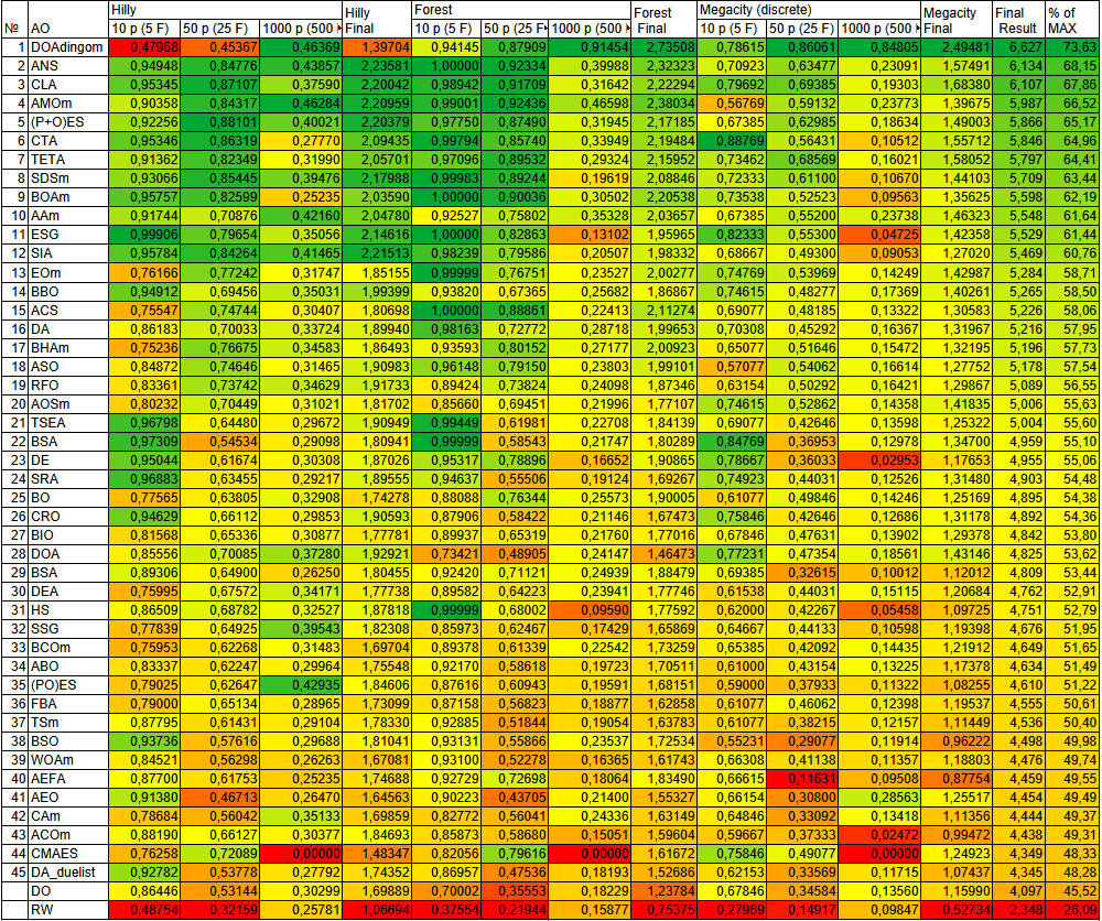
Figure 2. Color coding of algorithms across the corresponding tests
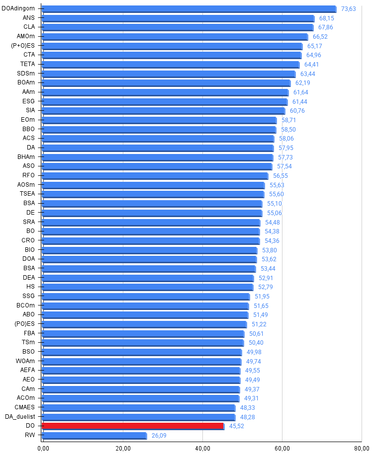
Figure 3. Histogram of algorithm test results (on a scale from 0 to 100; the higher the score, the better, where 100 is the maximum possible theoretical result; the archive contains a script for calculating the ranking table)
Pros and cons of the DO algorithm:
Pros:
- It handles certain types of problems well.
- Minimum external parameters: only the population size.
Cons:
- Unstable results on discrete functions.
- Slow.
An archive containing the current versions of the algorithm code is attached to the article. The author of this article is not responsible for the absolute accuracy of the descriptions of the canonical algorithms; many of them have been modified to improve their search capabilities. The conclusions and judgments presented in the articles are based on the results of the experiments conducted.
Programs used in the article
| # | Name | Type | Description |
|---|---|---|---|
| 1 | #C_AO.mqh | Include file | Parent class for population-based optimization algorithms |
| 2 | #C_AO_enum.mqh | Include file | Enumeration of population-based optimization algorithms |
| 3 | TestFunctions.mqh | Include file | Test function library |
| 4 | TestStandFunctions.mqh | Include file | Test bench function library |
| 5 | Utilities.mqh | Include file | Utility function library |
| 6 | CalculationTestResults.mqh | Include file | Script for calculating results for the comparison table |
| 7 | Testing AOs.mq5 | Script | Unified test bench for all population-based optimization algorithms |
| 8 | Simple use of population optimization algorithms.mq5 | Script | A simple example of using population-based optimization algorithms without visualization |
| 9 | Test_AO_DO.mq5 | Script | Test bench for DO |
Translated from Russian by MetaQuotes Ltd.
Original article: https://www.mql5.com/ru/articles/20540
Warning: All rights to these materials are reserved by MetaQuotes Ltd. Copying or reprinting of these materials in whole or in part is prohibited.
This article was written by a user of the site and reflects their personal views. MetaQuotes Ltd is not responsible for the accuracy of the information presented, nor for any consequences resulting from the use of the solutions, strategies or recommendations described.

 Reinforcement Learning Meets MetaTrader 5: A Complete Pipeline for Training, Validating and Honestly Evaluating a Gold Trading Bot
 Market Simulation: Position View (VII)
 Survival Analysis for Trade Exits: A Discrete-Time Competing-Risks Model in MQL5
 Combining LLM, CatBoost, and Quantum Computing into a Unified Trading System

- Free trading apps
- Over 8,000 signals for copying
- Economic news for exploring financial markets
You agree to website policy and terms of use
Hello.
Of course, here you go:
Articles
An advisor based on a universal MLP approximator
Andrey Dik, 13 December 2024 13:09
This article presents a simple and accessible way to use a neural network in a trading advisor, which does not require in-depth knowledge of machine learning. The method avoids normalising the objective function and eliminates the problems of ‘weight explosion’ and ‘network stagnation’, offering intuitive training and clear monitoring of results.Articles
Using optimisation algorithms to adjust an expert advisor’s parameters ‘on the fly’
Andrey Dik, 16 February 2024, 10:33
This article examines the practical aspects of using optimisation algorithms to find the best parameters for Expert Advisors ‘on the fly’, as well as the virtualisation of trading operations and Expert Advisor logic. This article can be used as a guide for implementing optimisation algorithms in a trading expert advisor.