Neural Networks in Trading: An End-to-End Multivariate Time Series Forecasting Model (Conclusion)

MetaTrader 5 — Trading systems | 3 September 2026, 07:31

450

Dmitriy Gizlyk

Introduction

In previous articles, we have progressed from an introduction to the theoretical aspects to the practical implementation of the proposed approaches, gradually revealing the architecture and logic of GinAR — an original neural network framework developed specifically for analyzing and forecasting time series under conditions of structural uncertainty and high noise levels. Built on a multilayer, multicomponent architecture, GinAR successfully combines attention mechanisms, graph transformations, and recurrent dynamics, thereby gaining the ability not only to perceive the structure of the data but also to adapt to it in real time.

We have now reached the most crucial — and perhaps the most interesting — part: evaluating the GinAR framework in real-world conditions. We have now completed the stages of architectural design, implementation of key components, and development of forward- and backward-pass algorithms. All components of the system have been thoroughly developed, tested, and adapted to the specific characteristics of financial time series. Now it is time to bring them all together and, as they say, put them through their paces — to see how effectively GinAR handles practical analysis and forecasting tasks.

In this article, we are not merely completing the development; we are marking the culmination of a concept whose implementation required considerable effort. The main focus will be on training and testing the model under conditions close to real-world deployment.

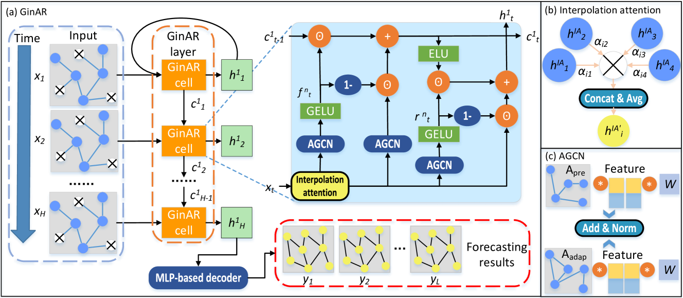
Before we move on to the evaluation, let's briefly review how the GinAR framework itself is structured. At its core is a custom cell, GinARCell, which combines several key components:

Interpolation Attention (IA) is a contextual attention mechanism that preprocesses the input stream and focuses the model on relevant elements. It is a kind of initial perception filter that makes it possible to identify significant patterns and reconstruct missing elements before the main transformation.
AGCN blocks (Adaptive Graph Convolution Network) consist of three modules, one of which is responsible for the main processing (cX_AGNC), while the other two handle control signals (ForgetGate and ResetGate). Their task is to extract structural and topological information, as well as to model the data flow based on temporal and structural dependencies.
The contextual block (Context) is a temporal state store that provides deep memory and continuity in the processing flow. Its state is updated according to a weighted scheme based on interaction with control gates (gates).
A dual control mechanism — ForgetGate and ResetGate — operates on the principles of filtering and overwriting the context. They are implemented as independent AGCN cells, which allows for flexible control of the model's internal state.

The cell's output is formed based on ELU activation and contextual attention multipliers, which ensures a smooth yet sensitive transition between time intervals.

This combination is what makes GinAR truly unique. Unlike classical recurrent neural networks, it does not just remember the past — it can structure it. Unlike standard GCN models, it does not operate on a fixed topology; instead, it learns the topology on the fly. Finally, unlike generalized transformers, GinAR preserves locality and dynamic adaptation — two features that are vital for analyzing financial time series.

An author’s visualization of the GinAR framework is shown below.

Author’s visualization of the GinAR framework

This article not only concludes the technical part but also serves as a demonstration of the maturity of the entire design. We will see how the framework performs in practice, what bottlenecks arise, and what accuracy and robustness the model achieves on new data. And, most importantly, we will assess whether it is truly capable of giving the trader the very edge that justifies all this architectural complexity.

GinAR Block

The GinAR architecture is organized hierarchically. It consists of several consecutive GinAR layers and ends with a Decoder built on a multilayer perceptron (MLP). Each GinAR layer, in turn, contains a set of GinARCell cells that process the temporal sequence step by step, much like the frames of a movie form a continuous scene.

At the output of each layer, only the final hidden state of the last cell is retained. These states are combined into a single final tensor, hⁿₐₗₗ, which contains a compressed and maximally informative representation of the entire sequence under analysis. It is this tensor that is fed into the MLP decoder, which consists of two fully connected layers with a ReLU activation function between them.

It is worth paying special attention to an important architectural aspect related to the organization of data flow in the multilayer structure of GinAR. In and of itself, the sequential application of several layers — where each subsequent layer receives the output of the previous one as its input — is a perfectly standard practice and fits well within the logic of the linear model.

However, the original GinAR model uses a more complex scheme: after sequential processing by several layers, the result is not simply the output of the last layer, but a combined representation obtained by concatenating the outputs of all layers. This approach allows the Decoder to use the entire spectrum of internal features generated at different levels of abstraction, which undoubtedly enhances the model. However, it also disrupts the linear data transfer structure that underlies our implementations and requires additional logic to collect and combine data from different layers.

The high-level model-building object we use did not originally support operations to merge the outputs of multiple layers into a single tensor, which makes it impossible to directly implement this part of the original GinAR architecture. To work around this limitation, we developed a special GinAR block that manages the sequential processing of the input data using a set of CNeuronGinARCell cells and then aggregates the results from all cells into a single tensor. This final tensor is fed into the Decoder, replicating a key feature of the original model — the integration of features obtained at different levels of abstraction.

As we turn to an examination of the architecture of the GinAR block, it is worth highlighting one important difference from the original model. In addition to the basic structure, we added a learnable matrix of predefined relationships between the components of the data being analyzed. It is based on an adaptive learning mechanism similar to the one used in the structural dependency matrices within each GinARCell cell. However, the key difference lies in the scope of application. While adaptive matrices are formed separately in each cell, reflecting local patterns, the matrix we introduced is global in nature and is shared by all cells within a single GinAR block. This makes it possible to capture stable, recurring correlations between variables throughout the analysis, thereby strengthening the model's structural consistency.

To implement the GinAR block within our architecture, we created a special class called CNeuronGinAR, which inherits from CNeuronSwiGLUOCL. This hierarchy allows us to maintain compatibility with the rest of the model and leverage the advantages of the underlying activation design together with the flexible SwiGLU nonlinearity. However, the key functional elements and operational logic were significantly expanded and redefined. The structure of the new object is shown below.

class CNeuronGinAR   :  public CNeuronSwiGLUOCL
  {
protected:
   CParams              cEa;
   CNeuronSwiGLUOCL     cWx;
   CNeuronSwiGLUOCL     cWe;
   CNeuronBaseOCL       cWconcat_ex;
   CNeuronConvOCL       cEn;
   CNeuronTransposeOCL  cEnT;
   CNeuronBaseOCL       cEnEnT;
   CNeuronSoftMaxOCL    cApre;
   CNeuronGinARCell     caCells[4];
   CNeuronBaseOCL       cConcat;
   //---
   virtual bool      feedForward(CNeuronBaseOCL *NeuronOCL) override;
   virtual bool      updateInputWeights(CNeuronBaseOCL *NeuronOCL) override;
   virtual bool      calcInputGradients(CNeuronBaseOCL *NeuronOCL) override;

public:
                     CNeuronGinAR(void) {};
                    ~CNeuronGinAR(void) {};
   //---
   virtual bool      Init(uint numOutputs, uint myIndex, COpenCLMy *open_cl,
                          uint units_count, uint dimension,
                          ENUM_OPTIMIZATION optimization_type, uint batch);
   //---
   virtual bool      Save(const int file_handle) override;
   virtual bool      Load(const int file_handle) override;
   //---
   virtual int       Type(void) override const  {  return defNeuronGinAR; }
   virtual void      TrainMode(bool flag) override;
   virtual void      SetOpenCL(COpenCLMy *obj);
   //---
   virtual bool      WeightsUpdate(CNeuronBaseOCL *source, float tau);
   //---
   virtual bool      Clear(void) override;
  };

The CNeuronGinAR class is a full-fledged block of the GinAR framework, implemented in the MQL5 environment using OpenCL. It is designed to process time series and extract complex patterns based on a hierarchy of linear relationships. The class brings together several key components responsible for generating and interpreting the global matrix of structural dependencies, as well as an array of CNeuronGinARCell cells that perform sequential processing of the input data. Their results are subsequently concatenated to form a final representation of the sequence being analyzed.

The class structure is based on the principles of modularity and reusability. All internal elements are declared statically. This means that their lifecycle management (creation, destruction, and memory cleanup) is handled automatically, without the need for explicit intervention from the constructor or destructor.

The Init method is used to configure all internal components; it serves as the single entry point for the initialization process. It accepts parameters that define the object's architecture and the type of parameter optimization.

bool CNeuronGinAR::Init(uint numOutputs, uint myIndex, COpenCLMy *open_cl,
                        uint units_count, uint dimension,
                        ENUM_OPTIMIZATION optimization_type, uint batch)
  {
   if(!CNeuronSwiGLUOCL::Init(numOutputs, myIndex, open_cl, caCells.Size()*dimension,
                              caCells.Size()*dimension, dimension, units_count, 1,
                              optimization_type, batch))
      return false;

First, the method of the same name from the parent class CNeuronSwiGLUOCL is called; in our implementation, it forms aggregated representations of the results produced by the GinARCell cells. After that, the newly declared components that are part of the block’s architecture are initialized sequentially.

The first is the learnable matrix of global structural dependencies between the time-series variables.

int index = 0;
if(!cEa.Init(0, index, OpenCL, Neurons(), optimization, iBatch))
   return false;
cEa.SetActivationFunction(None);

Unlike the original approach, in which a predefined covariance matrix is constructed based on prior knowledge or a preliminary analysis of the structure of the sequence being forecast, our implementation uses a learnable matrix of structural dependencies that is common to all GinARCell cells within a single block. This approach eliminates the need for manual tuning or external data analysis and enables more flexible, adaptive adjustment of the relationships between variables during the training phase.

Next, we initialize the linear transformation layers cWx and cWe. Their purpose is to map the input data and the covariance matrix to a common dimensionality before combining them into a single tensor cWconcat_ex.

   index++;
   if(!cWx.Init(0, index, OpenCL, dimension, dimension, dimension, units_count, 1,
                                                            optimization, iBatch))
      return false;
   index++;
   if(!cWe.Init(0, index, OpenCL, dimension, dimension, dimension, units_count, 1,
                                                            optimization, iBatch))
      return false;
   if(!cWconcat_ex.Init(0, index, OpenCL, 2 * Neurons(), optimization, iBatch))
      return false;
   cWconcat_ex.SetActivationFunction(None);

The cEn convolutional layer is designed to perform deep mixing of features and their dependencies.

   index++;
   if(!cEn.Init(0, index, OpenCL, 2 * dimension, 2 * dimension, dimension, units_count,
                                                              1, optimization, iBatch))
      return false;
   cEn.SetActivationFunction(None);
   index++;
   if(!cEnT.Init(0, index, OpenCL, units_count, dimension, optimization, iBatch))
      return false;
   index++;
   if(!cEnEnT.Init(0, index, OpenCL, units_count * units_count, optimization, iBatch))
      return false;
   cEnEnT.SetActivationFunction(GELU);

We first transpose the obtained data, and then multiply the original representation by its transpose to obtain a symmetric matrix of interdependencies between variables, cEnEnT. The GELU function is used for activation, enhancing significant relationships.

Next, we normalize the dependency matrix using the SoftMax function, converting the data into a probability distribution.

   index++;
   if(!cApre.Init(0, index, OpenCL, units_count * units_count, optimization, iBatch))
      return false;
   cApre.SetHeads(units_count);

The next step is to initialize an array of CNeuronGinARCell cells, each of which is responsible for processing the sequence being analyzed at its own level in the hierarchy. Despite their logical independence, all cells have an identical architecture, which simplifies the initialization process — a single well-structured loop is sufficient.

   for(uint i = 0; i < caCells.Size(); i++)
     {
      index++;
      if(!caCells[i].Init(0, index, OpenCL, units_count, dimension, optimization, iBatch))
         return false;
     }
   index++;
   if(!cConcat.Init(0, index, OpenCL, GetWindow()*units_count, optimization, iBatch))
      return false;
//---
   return true;
  }

The results from the cells are aggregated in the cConcat object. After successfully initializing all internal components, we return the boolean result of the operations to the calling program.

It is important to note that the Init method does not manage the lifecycle of the listed objects. Its task is to precisely configure the parameters and set up the layer architecture, then hand control over to the model's execution cycle. This approach ensures high stability, predictable behavior, and efficient memory usage.

Once the initialization phase is complete, all components of the CNeuronGinAR block are ready for operation during the forward pass. This is where the interaction among the structural modules, the hidden cell states, and the learnable matrix of dependencies becomes apparent. The feedForward method is responsible for executing the full processing cycle of the input sequence, including constructing the matrix of structural dependencies and generating the final output tensor, which will be passed to the next layer of the neural architecture.

bool CNeuronGinAR::feedForward(CNeuronBaseOCL *NeuronOCL)
  {
//--- Calculate Apre
   if(bTrain)
     {
      if(!cEa.FeedForward())
         return false;
      if(!cWe.FeedForward(cEa.AsObject()))
         return false;
     }

The first step involves constructing the learnable matrix of dependencies. If the model is in training mode (bTrain == true), the tensor of global structural dependencies is activated first, after which its output is processed by a linear projection layer.

In parallel, the main information flow of the input data is also processed as it passes through the cWx linear projection layer.

//---
   if(!cWx.FeedForward(NeuronOCL))
      return false;
   if(!Concat(cWx.getOutput(), cWe.getOutput(), cWconcat_ex.getOutput(), 
              cWx.GetWindowOut(), cWe.GetWindowOut(), cWx.GetUnits()))
      return false;

Next, the results from both branches are combined into a single tensor using the Concat operation, and the result is fed into the cEn convolutional layer.

   if(!cEn.FeedForward(cWconcat_ex.AsObject()))
      return false;
   if(!cEnT.FeedForward(cEn.AsObject()))
      return false;
   if(!MatMul(cEn.getOutput(), cEnT.getOutput(), cEnEnT.getOutput(), cEnT.GetCount(),
                                                  cEnT.GetWindow(), cEnT.GetCount()))
      return false;
   if(cEnEnT.Activation() != None)
      if(!Activation(cEnEnT.getOutput(), cEnEnT.getOutput(), cEnEnT.Activation()))
         return false;

The resulting tensor is then transposed (cEnT), after which the original tensor is multiplied by its transposed version. At this stage, a covariance matrix is effectively formed, and, if necessary, nonlinearity is added using the specified activation function.

The final covariance matrix is constructed in the cApre layer, where the data is converted into a probabilistic representation using the SoftMax function.

if(!cApre.FeedForward(cEnEnT.AsObject()))
   return false;
if(!IdentSum(cApre.getOutput(), cApre.getOutput(), cApre.Heads()))
   return false;

To ensure stability and a baseline level of self-connection, this matrix is supplemented with an identity matrix. In other words, each variable not only receives information about its relationships with the others, but also retains a basic self-reference. The result is a balanced structure of attention weights that can take into account both global dependencies and the local significance of each element. It is this final matrix that is then passed to the input of each GinARCell cell, serving as a universal mechanism for selective signal amplification.

Next, the main processing of the input sequence begins through the array of cells. The data to be analyzed, received from an external program, are fed into the input of the first cell. Each subsequent cell analyzes the results of the previous one, increasing the level of detail in the latent representation. Thus, a sequence of hidden representations is formed that reflects the hierarchical nature of time series analysis.

//--- GimAR Cells
   CNeuronBaseOCL *temp = NeuronOCL;
   for(uint i = 0; i < caCells.Size(); i++)
     {
      if(!caCells[i].FeedForward(temp, cApre.getOutput()))
         return false;
      temp = caCells[i].AsObject();
     }
//---
   if(!Concat(caCells[0].getOutput(), caCells[1].getOutput(), caCells[2].getOutput(),
              caCells[3].getOutput(), cConcat.getOutput(), GetWindow() / 4,
              GetWindow() / 4, GetWindow() / 4, GetWindow() / 4, GetUnits()))
      return false;
//---
   return CNeuronSwiGLUOCL::feedForward(cConcat.AsObject());
  }

The final step of the method is to combine the outputs of all cells into a single common tensor (cConcat), which is then passed as input to the method of the same name in the parent class CNeuronSwiGLUOCL for further processing. This structure ensures a coordinated and efficient flow of information through the GinAR block, bringing the system's behavior as close as possible to the original architecture despite the architectural limitations of the framework being used.

After completing the forward pass and computing the block's results, we move on to the second key stage: error gradient propagation (Backpropagation). This is where the true reverse engineering of forecasting begins: the error from the Decoder is fed back to each element of the architecture in order to precisely adjust the weights and optimize the model.

The calcInputGradients method is responsible for performing a complete backward pass through the entire block architecture, starting from the output and ending with the input data. Because the block's structure is complex and consists of both sequential operations and tensor branching and merging operations, the backward pass requires step-by-step and strictly coordinated execution.

bool CNeuronGinAR::calcInputGradients(CNeuronBaseOCL *NeuronOCL)
  {
   if(!NeuronOCL)
      return false;
//---
   if(!CNeuronSwiGLUOCL::calcInputGradients(cConcat.AsObject()))
      return false;
   if(!DeConcat(caCells[0].getPrevOutput(), caCells[1].getPrevOutput(),
                caCells[2].getPrevOutput(), caCells[3].getGradient(),
                cConcat.getGradient(), GetWindow() / 4,
                GetWindow() / 4, GetWindow() / 4,
                GetWindow() / 4, GetUnits()))
      return false;

The method begins by calling the method of the same name in the parent class CNeuronSwiGLUOCL, which passes the gradient to the concatenated tensor of the internal cells' outputs: cConcat. Since, during the forward pass, this tensor was formed by concatenating the outputs of four GinAR cells, it is now necessary to correctly distribute the gradient back across the four information streams. Using the DeConcat method, we pass the error gradient to each cell according to its impact on the final result.

One important point regarding the logic of error gradient propagation within the GinAR block deserves special emphasis. Despite the apparent symmetry of the cells, their functional roles during the learning process are not the same.

First, only the last cell is used solely to form the block's final result tensor through concatenation. All preceding cells serve a dual purpose: their outputs not only participate in concatenation but also serve as input data for the next GinARCell in the hierarchy. This means that the error gradient must enter each such cell from two sources. Therefore, when calculating the gradient for the first three cells, we collect the gradient along the two paths in which the data are used and sum them correctly. This ensures continuity of the error flow and accurate feedback at every level of the hierarchy.

//--- GimAR Cells
   cApre.getGradient().Fill(0);
   for(uint i = caCells.Size() - 1; i > 0; i--)
      if(!caCells[i - 1].CalcHiddenGradients(caCells[i].AsObject(), cApre.getOutput(),
                                             cApre.getPrevOutput(),
                                             (ENUM_ACTIVATION)cApre.Activation()) ||
         !SumAndNormilize(caCells[i - 1].getGradient(), caCells[i - 1].getPrevOutput(),
                          caCells[i - 1].getGradient(), cWx.GetWindow(), false, 0, 0, 0, 1) ||
         !SumAndNormilize(cApre.getGradient(), cApre.getPrevOutput(),
                          cApre.getGradient(), GetUnits(), false, 0, 0, 0, 1))
         return false;
   if(!NeuronOCL.CalcHiddenGradients(caCells[0].AsObject(), cApre.getOutput(),
                                     cApre.getPrevOutput(), (ENUM_ACTIVATION)cApre.Activation()) ||
      !SumAndNormilize(cApre.getGradient(), cApre.getPrevOutput(),
                       cApre.getGradient(), GetUnits(), false, 0, 0, 0, 1))
      return false;

Second, an even more nuanced situation arises when calculating the gradient for the global covariance matrix represented by the cApre object. This matrix was passed simultaneously to all four GinARCell instances. Consequently, during the backward pass, its gradient must accumulate information from four independent directions — from each cell. This requires adding all incoming gradients one by one while maintaining a consistent shape and scale. Errors in this part can lead to sharp jumps in the weights and, as a result, to unstable training.

Next, backpropagation begins through the dependency matrix formation block. First, the gradient for cEnEnT is calculated, after which the values are adjusted by the derivative of the corresponding activation function.

//---
   if(!cEnEnT.CalcHiddenGradients(cApre.AsObject()))
      return false;
   if(cEnEnT.Activation() != None)
      if(!DeActivation(cEnEnT.getOutput(), cEnEnT.getGradient(),
                       cEnEnT.getGradient(), cEnEnT.Activation()))
         return false;
   if(!MatMulGrad(cEn.getOutput(), cEn.getPrevOutput(),
                  cEnT.getOutput(), cEnT.getGradient(),
                  cEnEnT.getGradient(), cEnT.GetCount(),
                  cEnT.GetWindow(), cEnT.GetCount()))
      return false;
   if(!cEn.CalcHiddenGradients(cEnT.AsObject()))
      return false;
   if(!SumAndNormilize(cEn.getGradient(), cEn.getPrevOutput(),
                       cEn.getGradient(), cEnT.GetWindow(), false, 0, 0, 0, 1))
      return false;
   if(cEn.Activation() != None)
      if(!DeActivation(cEn.getOutput(), cEn.getGradient(),
                       cEn.getGradient(), cEn.Activation()))
         return false;

Next, the gradient for the MatMulGrad matrix multiplication operation is computed, thereby distributing the error between the convolutional layer cEn and its transposed copy cEnT. At the same time, we also propagate the error gradient of the transposed representation down to the convolutional layer and sum the values obtained from the two information flows. This approach makes it possible to construct a fully differentiable representation of the symmetric covariance matrix, thereby preserving the accuracy and integrity of error propagation even within a complex topology.

We propagate the obtained values down to the level of the cWconcat_ex tensor.

if(!cWconcat_ex.CalcHiddenGradients(cEn.AsObject()))
   return false;
if(!DeConcat(cWx.getGradient(), cWe.getGradient(), cWconcat_ex.getGradient(),
             cWx.GetWindowOut(), cWe.GetWindowOut(), cWx.GetUnits()))
   return false;

The cWconcat_ex output was formed from the results of cWx and cWe. Now their gradients are split back, passing through possible deactivation. After this, a backward pass is initiated from cWx to the source data object NeuronOCL.

However, we should remember here that the error gradient from the first cell had already been passed to the source data level. Therefore, we will use a trick involving the substitution of pointers to data buffers, followed by summing the values obtained from the two information flows.

   if(cWx.Activation() != None)
      if(!DeActivation(cWx.getOutput(), cWx.getGradient(),
                       cWx.getGradient(), cWx.Activation()))
         return false;
   if(cWe.Activation() != None)
      if(!DeActivation(cWe.getOutput(), cWe.getGradient(),
                       cWe.getGradient(), cWe.Activation()))
         return false;
   CBufferFloat* temp = NeuronOCL.getGradient();
   if(!NeuronOCL.SetGradient(NeuronOCL.getPrevOutput(), false))
      return false;
   if(!NeuronOCL.CalcHiddenGradients(cWx.AsObject()))
      return false;
   if(!SumAndNormilize(NeuronOCL.getGradient(), temp,
                       NeuronOCL.getGradient(), cWx.GetWindow(), false, 0, 0, 0, 1))
      return false;
   if(!NeuronOCL.SetGradient(temp, false))
      return false;

The method concludes by passing the error gradient to the level of the matrix of global dependencies cEa.

   if(!cEa.CalcHiddenGradients(cWe.AsObject()))
      return false;
//---
   return true;
  }

After all iterations have been completed successfully, we return the Boolean result of the method to the calling program.

Thus, the calcInputGradients method ensures correct gradient propagation throughout the entire structure of the GinAR block. The architecture of the backward pass exactly mirrors the structure of the forward pass, which is particularly important when using complex attention mechanisms and nested components.

The complete code for this class and all its methods is provided in the attachment and is available for independent study.

Model Architecture

Now that we have created all the components needed to build the GinAR framework, we move on to the next stage: describing the architecture of the trainable models. Here, the architecture goes far beyond simple time-series forecasting: our goal is to build a full-fledged trading agent in which the GinAR framework acts as the environment-state Encoder.

Each component of the model is responsible for a specific function. The Encoder is responsible for extracting and summarizing information from historical data. The forecasting modules, divided into three parallel models, perform forecasting over different time horizons. Next come the Actor and Critic, blocks corresponding to the Reinforcement Learning architecture: the former generates trading actions, while the latter evaluates the expected performance of the model's behavior in the current market state.

The CreateDescriptions method is used to describe the architecture; it generates configurations for all modules. In the first step, the method initializes containers for each model: the Encoder, forecasting modules, Actor, and Critic. These containers are implemented as arrays of objects, namely descriptions of neural layers.

bool CreateDescriptions(CArrayObj *&encoder,
                        CArrayObj *&forecast1,
                        CArrayObj *&forecast2,
                        CArrayObj *&forecast3,
                        CArrayObj *&actor,
                        CArrayObj *&critic
                       )
  {
//---
   CLayerDescription *descr;
//---
   if(!encoder)
     {
      encoder = new CArrayObj();
      if(!encoder)
         return false;
     }
   if(!forecast1)
     {
      forecast1 = new CArrayObj();
      if(!forecast1)
         return false;
     }
   if(!forecast2)
     {
      forecast2 = new CArrayObj();
      if(!forecast2)
         return false;
     }
   if(!forecast3)
     {
      forecast3 = new CArrayObj();
      if(!forecast3)
         return false;
     }
   if(!actor)
     {
      actor = new CArrayObj();
      if(!actor)
         return false;
     }
   if(!critic)
     {
      critic = new CArrayObj();
      if(!critic)
         return false;
     }

After initialization, the model structure begins to take shape. The Encoder starts with a basic fully connected layer that simply receives the model's historical input data.

//--- Encoder
   encoder.Clear();
//--- Input layer
   if(!(descr = new CLayerDescription()))
      return false;
   descr.type = defNeuronBaseOCL;
   uint prev_count = descr.count = (HistoryBars * BarDescr);
   descr.activation = None;
   descr.optimization = ADAM;
   if(!encoder.Add(descr))
     {
      delete descr;
      return false;
     }
//--- layer 1
   if(!(descr = new CLayerDescription()))
      return false;
   descr.type = defNeuronBatchNormWithNoise;
   descr.count = prev_count;
   descr.batch = BatchSize;
   descr.activation = None;
   descr.optimization = ADAM;
   if(!encoder.Add(descr))
     {
      delete descr;
      return false;
     }

Next comes a batch normalization layer with added noise, whose purpose is to stabilize the distribution of the raw data and introduce representation augmentation into the system to improve the model's robustness against overfitting.

After that, channels of differential features between adjacent bars are added. This allows the system to capture not only absolute values, but also the direction and intensity of changes. This is especially important under conditions of high-frequency and irregular market behavior.

//--- layer 2
   if(!(descr = new CLayerDescription()))
      return false;
   descr.type = defNeuronConcatDiff;
   prev_count = descr.count = HistoryBars;
   descr.layers = BarDescr;
   descr.step = 1;
   descr.batch = BatchSize;
   descr.optimization = ADAM;
   descr.activation = None;
   if(!encoder.Add(descr))
     {
      delete descr;
      return false;
     }

The next layer is responsible for enriching the representations with timestamp harmonics.

//--- layer 3
   if(!(descr = new CLayerDescription()))
      return false;
   descr.type = defMamba4CastEmbeding;
   prev_count = descr.count = HistoryBars;
   descr.window = 2 * BarDescr;
   uint prev_out = descr.window_out = NSkills;
     {
      uint temp[] = {PeriodSeconds(PERIOD_H1), PeriodSeconds(PERIOD_D1)};
      if(ArrayCopy(descr.windows, temp) < (int)temp.Size())
         return false;
     }
   descr.batch = BatchSize;
   descr.optimization = ADAM;
   descr.activation = None;
   if(!encoder.Add(descr))
     {
      delete descr;
      return false;
     }

The preprocessed data then pass through a transposition layer, which changes the representation axes: temporal sequences are transformed into spatial features and fed into a convolutional filter. A convolutional layer with tanh activation identifies key patterns and structural dependencies in the embeddings, thereby producing a compressed, concentrated representation of hidden market regularities.

//--- layer 4
   if(!(descr = new CLayerDescription()))
      return false;
   descr.type = defNeuronTransposeOCL;
   descr.count = prev_count;
   prev_count = descr.window = prev_out;
   descr.batch = BatchSize;
   descr.optimization = ADAM;
   descr.activation = None;
   if(!encoder.Add(descr))
     {
      delete descr;
      return false;
     }
   prev_out = descr.count;
//--- layer 5
   if(!(descr = new CLayerDescription()))
      return false;
   descr.type = defNeuronConvOCL;
   descr.count = prev_count;
   descr.window = prev_out;
   descr.variables = 1;
   prev_out = descr.window_out = EmbeddingSize;
   descr.batch = BatchSize;
   descr.optimization = ADAM;
   descr.activation = TANH;
   if(!encoder.Add(descr))
     {
      delete descr;
      return false;
     }

The culmination of the Encoder is the layer that implements the GinAR framework. It is here that all the previously obtained features are combined and interpreted using a hierarchy of GinAR cells. They operate synchronously, using a shared learnable covariance matrix to model hidden structural dependencies in the data. This layer does not merely pass information onward — it forms an active representation of the market state that can already be considered ready for use in making trading decisions.

//--- layer 6
   if(!(descr = new CLayerDescription()))
      return false;
   descr.type = defNeuronGinAR;
   descr.count = prev_count;
   descr.window = prev_out;
   descr.batch = BatchSize;
   descr.optimization = ADAM;
   descr.activation = None;
   if(!encoder.Add(descr))
     {
      delete descr;
      return false;
     }

Thus, the approaches of the GinAR framework are integrated into the model architecture consistently, logically, and without unnecessary complexity. The final hidden state formed by the Encoder is a high-level description of the market situation, suitable for both forecasting and generating trading decisions.

To train the environment state Encoder, a strategy of end-to-end error-gradient propagation from several independent subsystems at once is used. First and foremost, these are three forecasting models, each specializing in forecasting the continuation of the time series over its own planning horizon. These modules analyze the same hidden state generated by the Encoder, but interpret it differently depending on the specified planning horizon. This provides a multiscale understanding of the current market situation.

In addition, the Actor is added — a component responsible for generating a trading decision. It relies on the same compressed representation of the environment state and interprets it as a guide to action. Thus, the Encoder is under pressure from four directions at once: its output must be both informative for forecasting and suitable for practical application under market uncertainty.

It is important to emphasize that the architecture of all these models is borrowed entirely from the previous work. Therefore, in this study, we will not dwell on its detailed description. The focus is entirely on the new part — the integration of the GinAR framework into the trainable system.

The complete code for all components, including layer configurations, is provided in the attachment.

Training

Having completed the construction of all components and the configuration of the architecture of the trainable models, we move on to the final and perhaps most critical stage — model training. Within our system, we use a combined approach that brings together the strengths of both offline and online training modes. This not only ensures robust initial training of the model but also allows its behavior to be adapted to specific trading conditions, including changes in the market phase, volatility level, and the frequency of trading signals.

As in previous studies, the training process is implemented in two stages. The first stage is offline training. Here, the models are trained on historical data. Moreover, we use an approach that does not require collecting a training sample in advance. Instead, we construct the environment state directly from the terminal's historical data and simultaneously simulate the account state. This approach provides a high degree of flexibility and makes it possible to use arbitrary historical intervals without the need for manual dataset preparation.

The second stage is online fine-tuning. It is conducted under conditions that are as close as possible to live trading in the MetaTrader 5 Strategy Tester. The model continues training as it encounters new, previously unseen market scenarios and adapts to them in real time. This phase makes it possible to resolve residual mismatches accumulated during offline training and prepare the system for fully autonomous operation on a live account.

It is important to note that two-stage training is not a new concept in our research. We have successfully applied this strategy in our previous works as well. However, in the current project, during the offline training phase, fundamentally important changes were made, driven by both theoretical considerations and practical experience gained from implementing previous models.

You have probably noticed that the current architecture lacks a component called Director. Recall that in several recent works, the Director was used as an additional evaluation model operating in parallel with the Critic. Its main function was the binary classification of actions of the Agent as profitable or loss-making. This rigid form of feedback proved effective in the early stages of training, helping to accelerate the initial adaptation of the policy.

Nevertheless, in the current implementation we took a different approach. We therefore decided to combine two training approaches — reinforcement learning and supervised learning — directly in the offline training phase. This solution proved to be both more elegant and effective in terms of the quality and focus of the feedback.

The essence of the change is as follows: in parallel with the evaluation of the current actions of the Agent, which is performed by the Critic, we provide the Actor with reference actions derived from an analysis of future price movements. Since, during the offline training phase, we have access to the complete time-series segment, including subsequent price movements, we can calculate what is known as a near-perfect action trajectory. These actions, generated after the fact, do more than simply indicate the direction — they become a kind of reference point toward which the Actor's policy strives.

Thus, we implement a mechanism in which the Agent learns both from its own mistakes and from examples of precomputed profitable strategies. This makes it possible to move away from the harsh binary feedback from the Director without losing its training effect. On the contrary, the quality of the guiding signal improves, and the process of developing a profitable policy becomes more manageable and robust.

The proposed approach is implemented in the Train method of the Expert Advisor located at “…\MQL5\Experts\GinAR\Study.mq5”. This method's algorithm constitutes the central stage of offline training, combining reinforcement learning with supervised learning. It is based on the sequential simulation of market situations using historical data and on training a trading strategy by analyzing both current states and idealized trajectories of trading decisions.

It all starts with preparing a training dataset: a user-specified range is selected from the historical price data, and the technical indicators to be analyzed are calculated for each time interval. During this step, we ensure that all indicators have been calculated and are ready for use; otherwise, the process is interrupted.

void Train(void)
  {
   int start = iBarShift(Symb.Name(), TimeFrame, Start);
   int end = iBarShift(Symb.Name(), TimeFrame, End);
   int bars = CopyRates(Symb.Name(), TimeFrame, 0, start, Rates);
//---
   if(!RSI.BufferResize(bars) || !CCI.BufferResize(bars) ||
      !ATR.BufferResize(bars) || !MACD.BufferResize(bars))
     {
      PrintFormat("%s -> %d", __FUNCTION__, __LINE__);
      ExpertRemove();
      return;
     }
//---
   int count = -1;
   bool calculated = false;
   do
     {
      count++;
      calculated = (RSI.BarsCalculated() >= bars &&
                    CCI.BarsCalculated() >= bars &&
                    ATR.BarsCalculated() >= bars &&
                    MACD.BarsCalculated() >= bars
                   );
      Sleep(100);
      count++;
     }
   while(!calculated && count < 100);
   if(!calculated)
     {
      PrintFormat("%s -> %d The training data has not been loaded", __FUNCTION__, __LINE__);
      ExpertRemove();
      return;
     }
   RSI.Refresh();
   CCI.Refresh();
   ATR.Refresh();
   MACD.Refresh();
//---
   if(!ArraySetAsSeries(Rates, true))
     {
      PrintFormat("%s -> %d", __FUNCTION__, __LINE__);
      ExpertRemove();
      return;
     }
   bars -= end + HistoryBars + NForecast;
   if(bars < 0)
     {
      PrintFormat("%s -> %d", __FUNCTION__, __LINE__);
      ExpertRemove();
      return;
     }

Buffers are created to store input states, timestamps, and target values.

Next, the main training loop begins. Training is organized as a series of epochs — complete passes over the selected history. Within each epoch, market situations are simulated sequentially.

//---
   vector<float> result, target, neg_target;
   bool Stop = false;
//---
   uint ticks = GetTickCount();
//---
   for(int epoch = 0; (epoch < Epochs && !IsStopped() && !Stop); epoch ++)
     {
      if(!cEncoder.Clear())
        {
         PrintFormat("%s -> %d", __FUNCTION__, __LINE__);
         ExpertRemove();
         return;
        }
      for(int posit = start - HistoryBars - NForecast - 1; posit >= end; posit--)
        {
         if(!CreateBuffers(posit, GetPointer(bState), GetPointer(bTime), Result))
           {
            PrintFormat("%s -> %d", __FUNCTION__, __LINE__);
            ExpertRemove();
            return;
           }
         const vector<float> account = SampleAccount(GetPointer(bState), datetime(bTime[0]));
         const vector<float> target_action = OraculAction(account, Result);
         if(!bAccount.AssignArray(account))
           {
            PrintFormat("%s -> %d", __FUNCTION__, __LINE__);
            ExpertRemove();
            return;
           }

At each step, the current market state is formed as a numerical vector, and the corresponding time axis is determined. These data are fed into the Encoder, which transforms the state into a compact hidden representation — a kind of quintessence of the market picture.

//--- Feed Forward
if(!cEncoder.feedForward((CBufferFloat*)GetPointer(bState), 1, false,
                                   (CBufferFloat*)GetPointer(bTime)))
  {
   PrintFormat("%s -> %d", __FUNCTION__, __LINE__);
   Stop = true;
   break;
 }

The resulting latent vector is used in three ways simultaneously. On the one hand, it is fed into three forecasting models, each responsible for its own planning horizon: short-term, medium-term, and long-term. These models provide forecasts for the coming periods.

for(uint f = 0; f < caForecast.Size(); f++)
   if(!caForecast[f].feedForward(GetPointer(cEncoder), -1, (CBufferFloat*)NULL))
     {
      PrintFormat("%s -> %d - Forecast %d", __FUNCTION__, __LINE__, f);
      Stop = true;
      break;
     }

On the other hand, the same hidden representation is passed to the Actor, which is responsible for making the trading decision. Based on the market state and the current account state, it generates an action tensor.

if(!cActor.feedForward(GetPointer(bAccount), 1, false, GetPointer(cEncoder), LatentLayer))
  {
   PrintFormat("%s -> %d", __FUNCTION__, __LINE__);
   Stop = true;
   break;
  }

The decision made is evaluated by the Critic, which determines how reasonable it is under the given conditions.

if(!cCritic.feedForward(GetPointer(cActor), -1, GetPointer(cEncoder), LatentLayer))
  {
   PrintFormat("%s -> %d", __FUNCTION__, __LINE__);
   Stop = true;
   break;
  }

After performing a forward pass, we need to provide feedback to the models. First, the parameters of the forecasting models are adjusted.

//--- Study
for(uint f = 0; f < caForecast.Size(); f++)
   if(!caForecast[f].backProp(Result, (CBufferFloat*)NULL) ||
     !cEncoder.backPropGradient((CBufferFloat*)NULL))
     {
     PrintFormat("%s -> %d - Forecast %d", __FUNCTION__, __LINE__, f);
      Stop = true;
      break;
     }

The evaluation of the Actor's actions is based on calculating the reward: the change in equity normalized to the reference balance. In the event of a loss, the penalty is doubled to make the feedback stricter and more informative. We pass the resulting reward to the Critic. Then, from it, we backpropagate the error gradient to the Actor and the Encoder.

//---
cActor.getResults(Action);
double equity = bAccount[2] * bAccount[0] * EtalonBalance / (1 + bAccount[1]);
double reward = CheckAction(Action, equity, posit - NForecast + 1) / EtalonBalance;
if(reward < 0)
   reward *= 2;
Result.Clear();
if(!Result.Add(float(reward)))
  {
   PrintFormat("%s -> %d", __FUNCTION__, __LINE__);
   Stop = true;
   break;
  }
if(!cCritic.backProp(Result, GetPointer(cEncoder), LatentLayer) ||
  !cActor.backPropGradient(GetPointer(cEncoder), LatentLayer, -1, false) ||
  !cEncoder.backPropGradient((CBufferFloat*)NULL, NULL, LatentLayer, true))
 {
   PrintFormat("%s -> %d", __FUNCTION__, __LINE__);
   Stop = true;
  break;
  }

This is how the initial training takes place: based on the market's actual reaction to the selected action.

But the process does not end there. This is where the second part of the approach comes into play — supervised learning. Instead of relying solely on the market's actual response, the system uses information that is unavailable in real-world trading: knowledge of the future. For each state, a nearly perfect reference trajectory is calculated — the action that would have led to the best result, judging by the subsequent price movement. This action is passed to the Actor, which compares it with its own policy. In this way, we train the strategy not only through trial and error but also give it a clear benchmark to aim for. This two-layer scheme (actual and idealized control) accelerates learning and makes the model's behavior more stable and rational.

//--- Oracul
if(!Action.AssignArray(target_action))
  {
   PrintFormat("%s -> %d", __FUNCTION__, __LINE__);
   Stop = true;
   break;
  }
reward = CheckAction(Action, equity, posit - NForecast + 1) / EtalonBalance;
if(!cActor.backProp(Action, GetPointer(cEncoder), LatentLayer) ||
   !cEncoder.backPropGradient((CBufferFloat*)NULL, NULL, LatentLayer, true))
  {
   PrintFormat("%s -> %d", __FUNCTION__, __LINE__);
   Stop = true;
   break;
  }

The use of a reference action is not limited to training the Actor. We also pass this action to the input of the Critic, which — unlike in the first pass — evaluates behavior known to be correct. After the forward pass, the error is backpropagated to the Encoder using this idealized action. This allows the Critic to more accurately capture the structure of the reward function, obtain additional information about those regions of the state space where the Agent's behavior must be particularly precise, and, as a result, improve its effectiveness during subsequent training of the Actor.

if(!cCritic.feedForward(Action, 1, false, GetPointer(cEncoder), LatentLayer))
  {
   PrintFormat("%s -> %d", __FUNCTION__, __LINE__);
   Stop = true;
   break;
  }
if(!Result.Update(0, float(reward)))
  {
   PrintFormat("%s -> %d", __FUNCTION__, __LINE__);
   Stop = true;
   break;
  }
if(!cCritic.backProp(Result, GetPointer(cEncoder), LatentLayer) ||
   !cEncoder.backPropGradient((CBufferFloat*)NULL, NULL, LatentLayer, true))
  {
   PrintFormat("%s -> %d", __FUNCTION__, __LINE__);
   Stop = true;
   break;
  }
//---

This completes the full training cycle for a single state. Moreover, learning proceeds along two trajectories simultaneously: through actual behavior and through reference behavior. This dual-loop structure not only allows the error to be reduced more quickly but also helps form internal representations that are resilient to market noise and local fluctuations.

Throughout the entire procedure, a visual report is updated in the terminal at a specified frequency. The screen displays the average errors for all models. These data allow the developer to monitor training progress in real time, assess the stability of the process, and identify potential failures or anomalies.

    if(GetTickCount() - ticks > 500)
      {
       double percent = (epoch + 1.0 - double(posit - end) / 
                        (start - end - HistoryBars - NForecast))
                        / Epochs * 100.0;
       string str = "";
       for(uint f = 0; f < caForecast.Size(); f++)
          str += StringFormat("%-12s%d %6.2f%% -> Error %15.8f\n", "Forecast", f,
                                 percent, caForecast[f].getRecentAverageError());
       str += StringFormat("%-12s %6.2f%% -> Error %15.8f\n", "Actor", percent, 
                                                 cActor.getRecentAverageError());
       str += StringFormat("%-12s %6.2f%% -> Error %15.8f\n", "Critic", percent, 
                                                cCritic.getRecentAverageError());
       Comment(str);
       ticks = GetTickCount();
      }
   }
}

Once training across all epochs is complete, the algorithm summarizes the results — displaying the average error for each model. After that, the Expert Advisor shuts down.

   Comment("");
//---
   for(uint f = 0; f < caForecast.Size(); f++)
      PrintFormat("%s -> %d -> %-15s%d %10.7f", __FUNCTION__, __LINE__, "Forecast", f, 
                                               caForecast[f].getRecentAverageError());
   PrintFormat("%s -> %d -> %-15s %10.7f", __FUNCTION__, __LINE__, "Actor", 
                                                      cActor.getRecentAverageError());
   PrintFormat("%s -> %d -> %-15s %10.7f", __FUNCTION__, __LINE__, 
                                            "Critic",cCritic.getRecentAverageError());
   ExpertRemove();
//---
  }

Ultimately, the Train method shows how training a trading strategy can be structured by relying both on actual outcomes of actions and on ideal references derived from the future. This architecture provides not merely adaptation to past data, but a deliberate movement toward potential profit.

The complete code for this Expert Advisor, as well as for all the programs used in preparing this article, is included in the attachment.

Testing

As previously mentioned, the entire model training process was organized into two consecutive stages. In the first stage, we used offline training performed on historical data for the EURUSD currency pair with the H1 timeframe for the whole of 2024. This period encompasses a wide range of market scenarios — from prolonged sideways markets to rapid trending moves, and from sluggish, dormant periods to explosive spikes in volatility. This diversity allowed the model to encounter both typical and atypical situations, which is critical for reliability and versatility.

During training, the Encoder learned to identify recurring patterns in market information and compress them into a compact yet feature-rich representation. This internal market state became the foundation on which the Actor, using feedback from the Critic, formed a robust strategy capable of operating effectively under different conditions. In addition, during the offline training phase, the model was provided with so-called near-perfect trajectories — reference actions generated based on knowledge of future price movement. These cues not only steered the policy toward higher profits, but also provided a reliable reference point for building the strategy, especially in the early stages of training, when the model’s own experience was still limited.

After completing the offline training, we moved on to the second phase — online fine-tuning conducted under conditions close to the live market. Training was carried out in the MetaTrader 5 Strategy Tester, where the model analyzed the market in streaming mode, step by step and candle by candle. Not only did this allow us to test the model’s resilience to noise, market distortions, and random fluctuations, but it also became an important tool for adaptation: the model did not simply memorize — it actually learned to operate under real, unpredictable conditions. This approach significantly increased its robustness, reduced overfitting, and improved its generalization ability.

The final step was to test the model on entirely new data — market quotes for the period from January through March 2025. All parameters and internal settings used during training were retained unchanged. Thus, the results obtained allow for an objective assessment not only of the accuracy but also of the practical reliability of the proposed approach.

Test Results

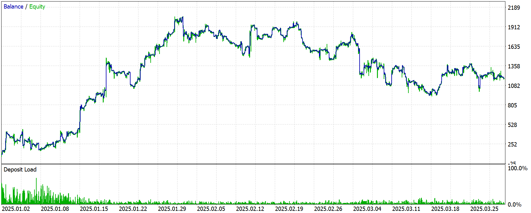
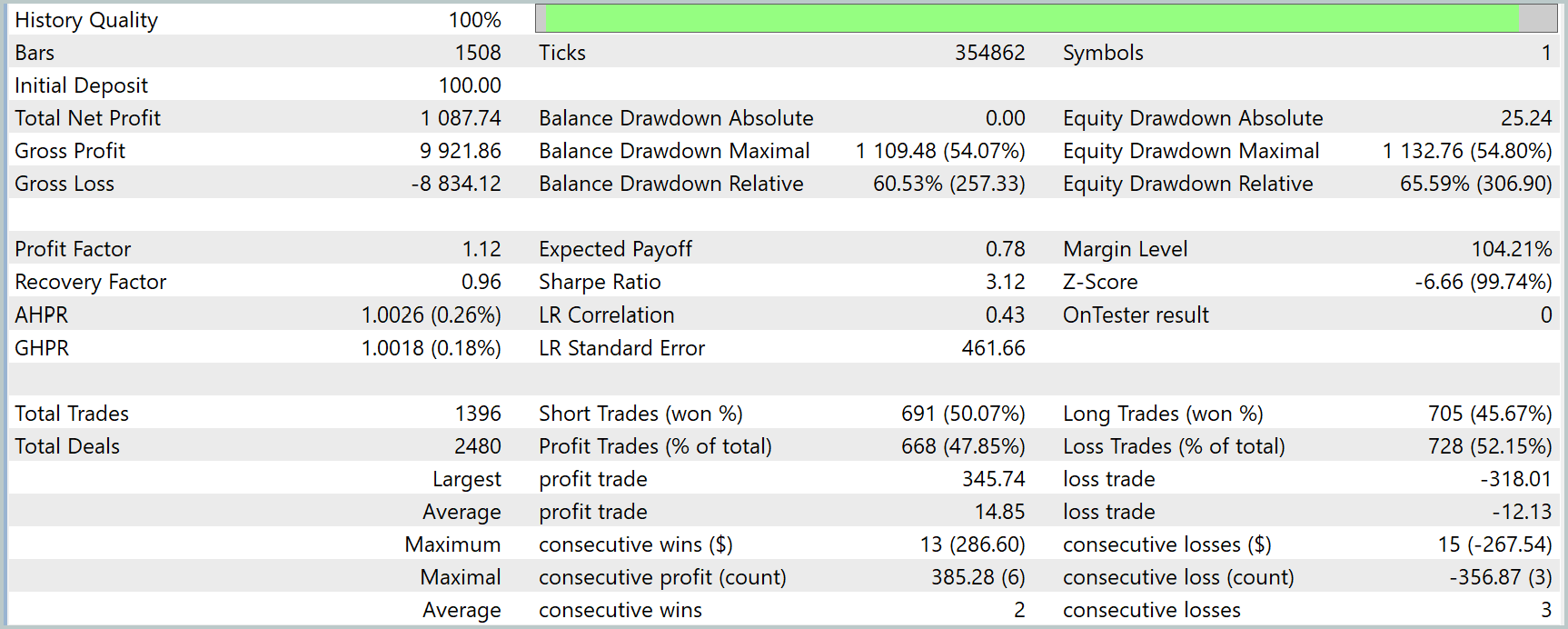
The model testing results provide an objective picture of its actual effectiveness and robustness outside the training sample. The initial deposit of $100 grew to $1,087.74, which is equivalent to a more than 10-fold increase in capital — a result that seems impressive at first glance. However, upon closer examination, a distinctive pattern becomes apparent: the model performs very well at the beginning of the test period, but as it moves further away from the training sample, its performance begins to decline.

The balance chart clearly illustrates this effect. The first third of the period is marked by rapid growth, following a near-reference trajectory with minimal drawdowns and steady gains. However, starting in mid-February and especially in March, the curve levels off and even shows signs of deterioration — fluctuations increase, losing streaks grow longer, and the rate of profit declines noticeably.

This effect is also confirmed by numerical metrics. The recovery factor (Recovery Factor) is less than 1 (0.96), which indicates a less-than-ideal ratio of profit to drawdown depth. The relative drawdown on equity reaches 65.59% — a fairly high level of risk, especially considering that the absolute drawdown at the start of the test was close to zero. The profit factor (Profit Factor) is 1.12 — the minimum acceptable value for a strategy that aims to operate consistently. The balance between profitable and unprofitable trades is also skewed against the model: profitable trades account for less than 48%.

This behavior can be logically explained by the limited size of the training sample. The model was trained using data from 2024 only, and although that data represented various market phases, the market remains a dynamic and volatile entity. As it moves further away from the known period, the model increasingly encounters situations with which it is unfamiliar. Without additional training episodes, its behavior becomes increasingly irrelevant, especially under new, volatile conditions.

One obvious way to solve this problem is to expand the training sample. Including data from previous years — for example, from 2020 or even 2015 — could enable the model to cover a much wider range of market scenarios. This will not only provide generalizability but also a better understanding of rare yet critically important price behavior patterns. Another option could be gradual online learning, with the model's weights updated periodically as new data arrive, which would keep the model up to date without full retraining.

Conclusion

In the course of our work, we demonstrated the practical applicability of the GinAR framework in real market conditions. From building the architecture and phased training to final testing, the entire process confirmed the viability of the proposed approach.

Despite strong performance at the beginning of the test period, the subsequent dynamics revealed the model's inherent limitations, which stemmed from the narrow training sample. This underscores a fundamental principle of working with time series: the robustness of a strategy depends directly on its ability to generalize knowledge beyond the training context.

The results obtained provide a solid foundation for further research and refinement. In particular, an obvious direction for further development is to expand the volume of training data and implement a continuous learning mechanism. All of this opens up opportunities for building truly adaptive and intelligent trading systems capable not only of surviving but also of consistently generating profits in challenging market conditions.

References

Programs used in the article

#	Name	Type	Description
1	Study.mq5	Expert Advisor	Expert Advisor for offline model training
2	StudyOnline.mq5	Expert Advisor	Expert Advisor for online model training
3	Test.mq5	Expert Advisor	Expert Advisor for model testing
4	Trajectory.mqh	Class Library	Structure for describing the system state and model architectures
5	NeuroNet.mqh	Class Library	Class library for creating a neural network
6	NeuroNet.cl	Library	Code library for the OpenCL program

Translated from Russian by MetaQuotes Ltd.
Original article: https://www.mql5.com/ru/articles/18914

Attached files |

Download ZIP

MQL5.zip (2935.06 KB)

Warning: All rights to these materials are reserved by MetaQuotes Ltd. Copying or reprinting of these materials in whole or in part is prohibited.

This article was written by a user of the site and reflects their personal views. MetaQuotes Ltd is not responsible for the accuracy of the information presented, nor for any consequences resulting from the use of the solutions, strategies or recommendations described.