

Harris Hawks Optimization (HHO)
 196
196
 2
2

Table of Contents
Introduction
When optimizing the parameters of a trading system within a limited computational budget (evaluation attempts), you inevitably face a dilemma: either the algorithm gets stuck too early in the first local optimum it finds, or it spends too much time exploring the space and fails to fully exploit promising regions by the end of the iteration budget. In practice, the transition point between exploration and exploitation is usually set manually using static hyperparameters — and this choice depends heavily on the specific task, the dimensionality, and the discretization grid. Given the limited number of calls to the fitness function and the “one fitness evaluation per iteration” rule, a mechanism is needed that automatically shifts the search from broad coverage to a targeted attack as the budget is consumed, without manual threshold adjustments.
Harris Hawks Optimization (HHO) offers precisely this approach: it is based on a scalar “escape energy” E, which deterministically decreases from ±2 to 0 as iterations progress, automatically switching the algorithm between the exploration and attack phases. In this article, we did not limit ourselves to a biological metaphor: we reproduced all HHO modes (two exploration variants, four attack strategies, including a Lévy-flight dive), adapted them to the unified MQL5 test bench interface with its requirement of one fitness evaluation per iteration, and implemented the working class C_AO_HHO. However, a technical limitation of the test bench (the inability to make two calls to the fitness function in a single iteration) forced us to replace the direct check F(Y) < F(X) in the Lévy strategy with a proxy rule based on the history of improvements — a detail that is important for the reproducibility and interpretation of the results.
The purpose of this article is to provide a ready-to-use component (Init/Moving/Revision, with the parameters popSize and β), a reproducible testing protocol (3 functions: Hilly, Forest, Megacity; three dimensionality levels; 10,000 calls per run; 10 repetitions), and an honest assessment of the applicability of HHO to practical tasks — in particular, to the calibration of trading systems under a limited budget.
Algorithm Implementation
The Texas deserts are home to a single species of bird of prey that hunts in flocks — the Harris's hawk. Several birds fan out, combing a wide area in search of a rabbit. As soon as prey is spotted, the tactics change instantly — the scouts transform into a well-coordinated team that closes in, cutting off all the prey’s escape routes. It is precisely this hunting behavior that is modeled by the Harris Hawks Optimization (HHO) algorithm, proposed by Heidari et al. in 2019.
Each hawk is a separate candidate solution to the optimization problem, a point X_i in the D-dimensional search space. The “rabbit” X_prey is the best solution found so far; this role is played by the cB[] vector of the global best. The algorithm controls how the hawks move — either individually exploring the space or collectively closing in on a find. In the implementation, each agent's next position is accumulated in the vector X_next (cP[]), then snapped to the search grid and passed to the fitness function.
A key innovation of HHO is the escape energy E, which decreases from ±2 to zero as the iterations are exhausted (Eq. 3):
E = 2 · E₀ · (1 − t / T)
E₀ ~ U(−1, 1) is a random initial energy, independent for each agent and each iteration; t is the current iteration number; T is the total number of iterations. The sign of E₀ specifies the direction of the rabbit's “struggle” for survival, and |E| determines the phase of the algorithm.
The parameter E functions as a timer that automatically switches the algorithm between two modes. As long as |E| ≥ 1, the hawks perform exploration, spreading out across the entire search space and acting independently. When |E| drops below 1, the search narrows and the hunt begins. An analogy: while there is still plenty of time left before the auction ends, participants examine a wide variety of lots throughout the room; as the timer nears zero, everyone's attention is focused on a single lot.
In exploration mode (|E| ≥ 1), each hawk chooses where to land in one of two ways, depending on a random parameter q ~ U(0, 1). When q < 0.5, a random neighbor X_rand from the current population serves as the reference point (Eq. 1a):
X_next[i] = X[rand] − r1 · |X[rand] − 2 · r2 · X[i]|;
where r1, r2 ~ U(0, 1) are independent for each coordinate, and X[rand] is the position of a randomly selected agent in the population. When q ≥ 0.5, the hawk uses the difference between the rabbit's position and the mean position of the population, X_mean (Eq. 2):
X_mean = (1/N) · Σ X[i]
and is shifted to an arbitrary location based on this difference (Eq. 1b):
X_next[i] = (X_prey − X_mean) − r3 · (LB + r4 · (UB − LB)); r3, r4 ~ U(0, 1);
LB, UB are the lower and upper search bounds. X_mean is calculated once as a snapshot at the start of the iteration—all agents see the same mean, which eliminates any dependence on the order of updates. Both options ensure a wide spread of agents, reducing the risk of getting stuck in a local optimum.
When the rabbit is detected (|E| < 1), four attack strategies come into play. Their choice depends on two factors: how exhausted the rabbit is and whether it has managed to break free. Exhaustion is determined by |E|: when |E| ≥ 0.5, the rabbit is still energetic; when |E| < 0.5, it is running out of energy. The success of the escape is determined by a random parameter r ~ U(0, 1), which is independent of E.
Soft besiege (r ≥ 0.5, |E| ≥ 0.5) — the hawks gradually close the distance, like firefighters methodically pushing back a fire (Eq. 4):
X_next[i] = (X_prey − X[i]) − E · |J · X_prey − X[i]|
J = 2 · (1 − U(0,1)) is the magnitude of the rabbit's random leap in an attempt to break free; the difference X_prey − X[i] is the closing-in vector. Hard besiege (r ≥ 0.5, |E| < 0.5) — the rabbit is exhausted; a direct attack without flanking maneuvers (Eq. 6):
X_next[i] = X_prey − E · |X_prey − X[i]|
J is not used in this strategy — the rabbit is no longer capable of active maneuvering.
A Lévy flight is not quite an ordinary random walk. Most steps are small, but occasionally there is a jump dozens of times longer. This distribution is found throughout nature — from the flight paths of albatrosses to the movements of molecules. The Lévy step is calculated using Mantegna's formula (Eq. 9):
LF = u / |v|^(1/β), u ~ N(0, σ²), v ~ N(0, 1)
σ = [Γ(1+β)·sin(πβ/2) / (Γ((1+β)/2)·β·2^((β−1)/2))]^(1/β); where β = 1.5 is the distribution tail index, a constant; u and v are independent normal samples generated using the Box–Muller method; σ is precomputed once in Init(). The LF result is signed: u can be negative, which ensures that the jump is bidirectional.
In HHO, the Lévy flight is used in strategies 3 and 4 as a fallback maneuver: if a directed move toward the rabbit does not improve the hawk’s position, a random Lévy perturbation is added. Soft besiege with diving (r < 0.5, |E| ≥ 0.5) — the rabbit is still full of energy and zigzags; the hawk first tries the directed step Y and, if that fails, adds a Lévy perturbation (Eq. 7–10):
Y = X_prey − E · |J · X_prey − X[i]|
Z = Y + U(0,1) · LF(D)
X_next[i] = Y if F(Y) < F(X[i]), otherwise Z.
Hard besiege with a dive (r < 0.5, |E| < 0.5) — the rabbit is exhausted; the attack is oriented toward the flock's center of mass, X_mean, rather than the agent’s individual position (Eq. 11–13):
Y = X_prey − E · |J · X_prey − X_mean|
Z = Y + U(0,1) · LF(D)
X_next[i] = Y if F(Y) < F(X[i]), otherwise Z.
Selecting Y or Z requires two calls to the fitness function within a single iteration. In this implementation, the framework allows exactly one fitness evaluation per iteration, so a proxy criterion is used: if the agent improved in the previous iteration (f[i] > f_prev[i]), Y is used; otherwise, Z is used. In the first iteration, f_prev[i] = −∞, which guarantees the selection of Z and promotes initial diversity through Lévy jumps.
Like a detective who methodically searches a room but sometimes, on a hunch, dashes up to another floor: most of those detours will turn out to be fruitless, but one of them might uncover a solution that a systematic search would have missed. This is precisely the role of strategies 3 and 4: the Lévy jump as a safeguard against premature convergence. The concept behind the algorithm is illustrated in the figure below.
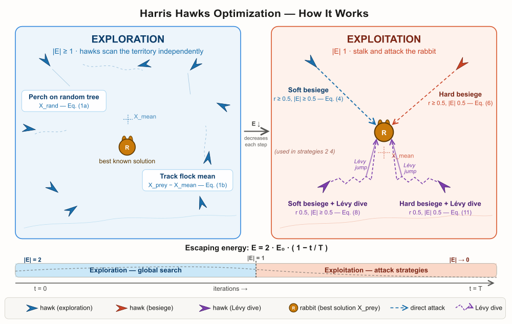
Figure 1. Illustration of how the HHO algorithm works
The illustration contains all the key elements of the algorithm. The left panel shows the exploration phase: 9 hawks fly off in random directions throughout the space; the rabbit is present but is not the focus of attention. The right panel shows the exploitation phase: 4 hawks attack the rabbit, each using its own strategy — straight blue arrows for strategies 1 and 2 (soft besiege and hard besiege), purple zigzags for strategies 3 and 4 (besiege + Lévy-flight dive; the long jump at the end of the path is intentionally highlighted). The timeline at the bottom shows E decreasing from 2 to 0, with a decay curve and a clear boundary at |E| = 1.
Let's move on to writing the pseudocode for HHO.
Init
INIT(LB[], UB[], step[], epochsP):
t ← 0 ; T ← epochsP
// Eq. (9): σ — precomputed once using LGamma()
num ← exp(LGamma(1+β)) · sin(π·β/2)
den ← exp(LGamma((1+β)/2)) · β · 2(β−1)/2
σ ← (den > 1e-15) ? (num/den)1/β : 1 // σ for LevyStep()
for i = 0..N−1:
for c = 0..D−1: X_next[i][c] ← U(LB[c], UB[c]) // random initialization
f_prev[i] ← −∞ // → the first iteration always selects Z (Lévy)
Moving · called before every fitness calculation
MOVING():
for i = 0..N−1:
for c = 0..D−1: X[i][c] ← snap(X_next[i][c], LB[c], UB[c], step[c])
Revision · called after calculating f[i] = F(X[i]) by the external code
REVISION():
t ← t + 1
// ─── 1. Updating personal bests and the global best ─────────────
for i = 0..N−1:
if f[i] > f_best[i]: f_best[i] ← f[i] ; X_best[i] ← X[i]
if f[i] > f_prey: f_prey ← f[i] ; X_prey ← X[i] // “rabbit”
// ─── 2. Mean position of the flock/population over X[i] (snapshot) ── Eq. (2) ──
for c = 0..D−1: X_mean[c] ← (1/N) · Σᵢ X[i][c]
// ─── 3. Overall energy multiplier for the iteration ──────────────
E1 ← 2 · (1 − t / T)
// ─── 4. Updating the position of each hawk ───────────────────
for i = 0..N−1:
// [L3] proxy for “Y is better than X” — set this value BEFORE updating f_prev
improvedLast ← (f[i] > f_prev[i])
f_prev[i] ← f[i]
// Eq. (3): E = E1 · E0, E0 ~ U(−1, 1) — inline; no separate variable is needed
E ← E1 · (2 · U(0,1) − 1)
|E| ← |E|
if |E| ≥ 1: // ══ EXPLORATION ══
q ← U(0,1) // is generated only in this branch
if q < 0.5: // Eq. (1a): random tree — orientation toward X[ri]
ri ← randInt(0, N−1)
r1, r2 ← U(0,1)
for c = 0..D−1:
X_next[i][c] ← clamp( X[ri][c] − r1·|X[ri][c] − 2·r2·X[i][c]|, LB[c], UB[c] )
else: // q ≥ 0.5 — Eq. (1b): orientation from X_prey through X_mean
r3, r4 ← U(0,1)
for c = 0..D−1:
X_next[i][c] ← clamp( (X_prey[c] − X_mean[c]) − r3·(LB[c] + r4·(UB[c]−LB[c])), LB[c], UB[c] )
else if |E| < 1 and r ≥ 0.5 and |E| ≥ 0.5: // ── Strategy 1: soft besiege ──
r ← U(0,1) // is generated first in the exploitation block
J ← 2·(1 − U(0,1)) // Jump_strength
for c = 0..D−1: // Eq. (4), ΔX = X_prey − X[i] (Eq. (5), inline)
X_next[i][c] ← clamp( (X_prey[c]−X[i][c]) − E·|J·X_prey[c] − X[i][c]|, LB[c], UB[c] )
else if |E| < 1 and r ≥ 0.5 and |E| < 0.5: // ── Strategy 2: hard besiege ──
// J is not needed in this strategy
for c = 0..D−1: // Eq. (6)
X_next[i][c] ← clamp( X_prey[c] − E·|X_prey[c] − X[i][c]|, LB[c], UB[c] )
else if |E| < 1 and r < 0.5 and |E| ≥ 0.5: // ── Strategy 3: soft besiege + Lévy ──
J ← 2·(1 − U(0,1))
for c = 0..D−1: // Eq. (7) — candidate Y
Y[c] ← clamp( X_prey[c] − E·|J·X_prey[c] − X[i][c]|, LB[c], UB[c] )
if improvedLast: // proxy F(Y) < F(X[i]) → take Y [L3]
X_next[i] ← Y
else: // proxy F(Y) ≥ F(X[i]) → Z = Y + Lévy Eq. (8)
for c = 0..D−1:
Z[c] ← clamp( Y[c] + U(0,1) · LevyStep(), LB[c], UB[c] ) // rand·LF(D)
X_next[i] ← Z
else: // |E| < 1, r < 0.5, |E| < 0.5 ── Strategy 4: hard besiege + Lévy ──
J ← 2·(1 − U(0,1))
for c = 0..D−1: // Eq. (12) — candidate Y' (X_mean instead of X[i])
Y[c] ← clamp( X_prey[c] − E·|J·X_prey[c] − X_mean[c]|, LB[c], UB[c] )
if improvedLast: // proxy F(Y') < F(X[i]) → take Y' [L3]
X_next[i] ← Y
else: // proxy F(Y') ≥ F(X[i]) → Z' = Y' + Lévy Eq. (13)
for c = 0..D−1:
Z[c] ← clamp( Y[c] + U(0,1) · LevyStep(), LB[c], UB[c] )
X_next[i] ← Z
// end strategy selection
// end for i
return X_prey, f_prey
LevyStep · signed scalar step — per-coordinate is called
LevyStep() → double:
// Box-Muller: two independent N(0,1) variables drawn from a single pair of uniformly distributed numbers
r1 ← U(1e-15, 1), r2 ← U(0, 1) // r1 > 0 so that ln(r1) does not blow up
n1 ← √(−2·ln r1) · cos(2π·r2) // n1 ~ N(0, 1)
n2 ← √(−2·ln r1) · sin(2π·r2) // n2 ~ N(0, 1)
u ← n1 · σ // u ~ N(0, σ²), as in randn()*sigma in the original
v ← n2 // v ~ N(0, 1), as in randn() in the original
av ← max(|v|, 1e-15)
return u / av1/β // signed result — preserves the sign of u and provides the ±direction
Now we can move on directly to the implementation.
The C_AO_HHO class inherits from the base class C_AO, which provides a unified test bench interface: an array of agents a[], a global best vector cB[], the counters coords and popSize, and the helper object "u" with random number generators. The class’s private fields "t" and "T" store the current iteration and the maximum number of iterations; they are needed to calculate the decreasing energy E1 = 2·(1 − t/T). The sigma field is calculated once in Init() and is used by the LevyStep() function throughout the entire run. The temporary buffers Xm[] and Ytmp[] are allocated for coords elements during initialization and reused without reallocating memory.
//────────────────────────────────────────────────────────────────────
class C_AO_HHO : public C_AO
{
  public: //------------------------------------------------------------
  ~C_AO_HHO () { }
  C_AO_HHO ()
  {
    ao_name = "HHO";
    ao_desc = "Harris Hawks Optimization";
    ao_link = "https://www.mql5.com/en/articles/21898";

    popSize = 50;
    beta    = 1.5;

    ArrayResize (params, 2);
    params [0].name = "popSize"; params [0].val = popSize;
    params [1].name = "beta";    params [1].val = beta;
  }

  void SetParams ()
  {
    popSize = (int)params [0].val;
    beta    =      params [1].val;
  }

  bool Init (const double &rangeMinP  [],
             const double &rangeMaxP  [],
             const double &rangeStepP [],
             const int     epochsP = 0);

  void Moving   ();
  void Revision ();

  //------------------------------------------------------------------
  double beta; // Lévy tail index (β = 1.5 in the original)

  private: //---------------------------------------------------------
  int    t;      // current iteration (starting at 1)
  int    T;      // total number of iterations
  double sigma;  // σ for the Lévy formula (Eq. 9), calculated once in Init

  double Xm   []; // [coords]  mean position of the flock (Eq. 2)
  double Ytmp []; // [coords]  candidate Y  (strategies 3, 4)

  double LGamma   (double x); // logarithm of Γ(x), Lanczos approximation
  double LevyStep ();         // [L2] scalar Lévy step: u~N(0,σ), v~N(0,1)

  double Clamp (double v, double lo, double hi)
  {
    return v < lo ? lo : (v > hi ? hi : v);
  }
};
//————————————————————————————————————————————————————————————————————
The Init() method performs a complete reset of the algorithm's state before each test run. It calls StandardInit(), which allocates the array of agents, copies the range bounds, and resets the random number generator. It then stores `epochsP` as "T", resets the "t" counter, and allocates the buffers. The sigma precomputation is performed using Mantegna's formula (Eq. 9): numerator — Γ(1+β)·sin(πβ/2), denominator — Γ((1+β)/2)·β·2^((β-1)/2); the result is raised to the power of 1/β. The computation is delegated to LGamma() to avoid overflow when the gamma function is computed directly via the factorial. Each agent is initialized uniformly in [LB, UB], and the field a[i].fP is reset to −DBL_MAX — this ensures that on the first iteration, improvedLast = false, and strategies 3 and 4 will always choose the branch with a Lévy jump, thereby promoting initial diversity.
//————————————————————————————————————————————————————————————————————
bool C_AO_HHO::Init (const double &rangeMinP  [],
                     const double &rangeMaxP  [],
                     const double &rangeStepP [],
                     const int     epochsP = 0)
{
  if (!StandardInit (rangeMinP, rangeMaxP, rangeStepP)) return false;

  //------------------------------------------------------------------
  T = (epochsP > 0) ? epochsP : 1;
  t = 0;

  ArrayResize (Xm,   coords);
  ArrayResize (Ytmp, coords);

  //--- Eq. (9): σ = [Γ(1+β)·sin(πβ/2) / (Γ((1+β)/2)·β·2^((β-1)/2))]^(1/β)
  double num = exp (LGamma (1.0 + beta)) * sin (M_PI * beta * 0.5);
  double den = exp (LGamma ((1.0 + beta) * 0.5)) * beta * pow (2.0, (beta - 1.0) * 0.5);
  sigma = (den > 1e-15) ? pow (fabs (num / den), 1.0 / beta) : 1.0;

  //--- initial positions: uniformly random in [LB, UB]
  for (int i = 0; i < popSize; i++)
  {
    for (int c = 0; c < coords; c++)
    {
      a [i].cP [c] = u.RNDfromCI (rangeMin [c], rangeMax [c]);
    }
    a [i].fP = -DBL_MAX; // Reset the improvement history for [L3]
  }

  return true;
}
//————————————————————————————————————————————————————————————————————
The Moving() method transfers the projected positions from cP[] to c[] by snapping them to a discrete grid via SeInDiSp(). It is called by the test bench before each fitness-function calculation. All the logic for computing the next step is concentrated in `Revision()`; `Moving()` is solely a projection operation.
//————————————————————————————————————————————————————————————————————
void C_AO_HHO::Moving ()
{
  for (int i = 0; i < popSize; i++)
  {
    for (int c = 0; c < coords; c++)
    {
      a [i].c [c] = u.SeInDiSp (a [i].cP [c], rangeMin [c], rangeMax [c], rangeStep [c]);
    }
  }
}
//————————————————————————————————————————————————————————————————————
The Revision() method is the main method and is called by the test bench after the external code has calculated the fitness of all agents and stored the results in a[i].f. It performs four consecutive steps. First, the best positions are updated: for each agent, the current fitness is compared with its personal best a[i].fB and with the global best fB; if an improvement is found, the corresponding coordinate vectors are copied. The vector cB[] always stores the rabbit's position. The second step is to calculate the mean position of the flock, Xm[] (Eq. 2) based on the current coordinates a[i].c[]. The third step is to compute E1 = 2·(1 − t/T), an iteration-wide decreasing multiplier. The fourth step is to update the position of each hawk.
At the beginning of the block, the proxy flag `improvedLast = (a[i].f > a[i].fP)` is set, after which `fP` is updated for the next iteration. This flag replaces the double fitness-function call used in the original in strategies 3 and 4: if the agent improved in the previous iteration, we trust the directed step Y; if not, we add the Lévy perturbation Z. Random numbers E, q, or r — and J, if necessary — are generated strictly within the branch of code where they are needed, without unnecessary calls to the random number generator.
The Clamp() helper method limits the value of v to the interval [lo, hi] and is applied after each calculation of the agent’s new position, ensuring that the candidate vector cP[] remains within the valid search range regardless of the step size — including potentially large Lévy jumps.
//————————————————————————————————————————————————————————————————————
// Revision(): updates X_prey and X_m, and computes cP for the next step.
//
// The structure matches the original:
//   |E| ≥ 1 → exploration:
//       q < 0.5  → X_rand formula (Eq. 1a)      [L1]
//       q ≥ 0.5 → X_prey − X_m  (Eq. 1b)
//   |E| <  1 → exploitation:
//       r ≥ 0.5, |E| ≥ 0.5 → strategy 1: soft besiege          Eq. (4-5)
//       r ≥ 0.5, |E| < 0.5 → strategy 2: hard besiege         Eq. (6)
//       r < 0.5, |E| ≥ 0.5 → strategy 3: soft besiege + Lévy  Eq. (7-10)
//       r < 0.5, |E| < 0.5 → strategy 4: hard besiege + Lévy Eq. (11-13)
//
// [L3] In the original, strategies 3/4 make two fobj calls (for Y and Z).
//      Proxy in our framework: if the agent improved in the previous iteration
//      (a[i].f > a[i].fP) — we trust the directed step Y;
//      otherwise, we add Lévy → Z (as a fallback).
void C_AO_HHO::Revision ()
{
  t++;

  //─── 1. Updating personal and global bests ──────────────────
  for (int i = 0; i < popSize; i++)
  {
    if (a [i].f > a [i].fB)
    {
      a [i].fB = a [i].f;
      ArrayCopy (a [i].cB, a [i].c, 0, 0, coords);
    }
    if (a [i].f > fB)
    {
      fB = a [i].f;
      ArrayCopy (cB, a [i].c, 0, 0, coords);
    }
  }

  //─── 2. Mean position of the flock Xm (Eq. 2) ───────────────────────
  ArrayInitialize (Xm, 0.0);
  for (int i = 0; i < popSize; i++)
  {
    for (int c = 0; c < coords; c++)
    {
      Xm [c] += a [i].c [c];
    }
  }
  for (int c = 0; c < coords; c++)
  {
    Xm [c] /= (double)popSize;
  }

  //─── 3. E1 — common to the entire iteration  ─────────────
  double E1 = 2.0 * (1.0 - (double)t / (double)T);

  //─── 4. Update of each hawk's position ──────────────────────
  for (int i = 0; i < popSize; i++)
  {
    //--- [L3] Record the improvement flag BEFORE updating fP
    bool improvedLast = (a [i].f > a [i].fP);
    a [i].fP = a [i].f; // Save this for the next iteration

    //--- Eq. (3): E = E1·E0, E0 ~ U(−1,1)  [E0 is not needed separately]
    double E    = E1 * (2.0 * u.RNDfromCI (0.0, 1.0) - 1.0);
    double absE = fabs (E);

    if (absE >= 1.0)
    {
      //══ EXPLORATION ══════════════════════════════════════════════
      // q is generated only here
      double q = u.RNDfromCI (0.0, 1.0);

      if (q < 0.5)
      {
        //─ [L1] Eq. (1a): orientation toward a random flock member ──────
        //  Xi(t+1) = X_rand − r1·|X_rand − 2·r2·Xi|
        int    ri = u.RNDminusOne (popSize);
        double r1 = u.RNDfromCI (0.0, 1.0);
        double r2 = u.RNDfromCI (0.0, 1.0);
        for (int c = 0; c < coords; c++)
        {
          a [i].cP [c] = Clamp (a [ri].c [c] - r1 * fabs (a [ri].c [c] - 2.0 * r2 * a [i].c [c]), rangeMin [c], rangeMax [c]);
        }
      }
      else
      {
        //─ Eq. (1b): orientation toward the difference X_prey − X_m ───────────
        //  Xi(t+1) = (X_prey − X_m) − r3·((UB−LB)·r4 + LB)
        double r3 = u.RNDfromCI (0.0, 1.0);
        double r4 = u.RNDfromCI (0.0, 1.0);
        for (int c = 0; c < coords; c++)
        {
          a [i].cP [c] = Clamp ((cB [c] - Xm [c]) - r3 * (rangeMin [c] + r4 * (rangeMax [c] - rangeMin [c])), rangeMin [c], rangeMax [c]);
        }
      }
    }
    else
    {
      //══ EXPLOITATION ═══════════════════════════════════════════════
      // r is generated only here
      double r = u.RNDfromCI (0.0, 1.0);

      if (r >= 0.5 && absE >= 0.5)
      {
        //─ Strategy 1: soft besiege ─────────────────────────────────
        //  ΔX = X_prey − Xi                                   Eq. (5)
        //  Xi(t+1) = ΔX − E·|J·X_prey − Xi|                  Eq. (4)
        //  J is generated here (Jump_strength)
        double J = 2.0 * (1.0 - u.RNDfromCI (0.0, 1.0));
        for (int c = 0; c < coords; c++)
        {
          a [i].cP [c] = Clamp ((cB [c] - a [i].c [c]) - E * fabs (J * cB [c] - a [i].c [c]), rangeMin [c], rangeMax [c]);
        }
      }
      else
      {
        if (r >= 0.5 && absE < 0.5)
        {
          //─ Strategy 2: hard besiege ────────────────────────────────
          //  Xi(t+1) = X_prey − E·|X_prey − Xi|                Eq. (6)
          //  J is not used in this strategy
          for (int c = 0; c < coords; c++)
          {
            a [i].cP [c] = Clamp (cB [c] - E * fabs (cB [c] - a [i].c [c]), rangeMin [c], rangeMax [c]);
          }
        }
        else
        {
          if (r < 0.5 && absE >= 0.5)
          {
            //─ Strategy 3: soft besiege + Lévy-flight dive ──────────────
            //  Y = X_prey − E·|J·X_prey − Xi|                    Eq. (7)
            //  Z = Y + rand·LF(D)                                 Eq. (8)
            //  Xi = Y if F(Y) < F(Xi), otherwise Z if F(Z) < F(Xi),
            //          otherwise Xi remains unchanged (stay-put is not supported by the framework).
            //  [L3] proxy: improvedLast → Y; otherwise → Z.
            //  J is generated here
            double J = 2.0 * (1.0 - u.RNDfromCI (0.0, 1.0));
            for (int c = 0; c < coords; c++)
            {
              Ytmp [c] = Clamp (cB [c] - E * fabs (J * cB [c] - a [i].c [c]), rangeMin [c], rangeMax [c]);
            }

            if (improvedLast)
            {
              for (int c = 0; c < coords; c++) a [i].cP [c] = Ytmp [c];
            }
            else
            {
              // Z = Y + rand·LF(D), rand(1,dim).*Levy(dim)  [L2]
              for (int c = 0; c < coords; c++)
              {
                a [i].cP [c] = Clamp (Ytmp [c] + u.RNDfromCI (0.0, 1.0) * LevyStep (), rangeMin [c], rangeMax [c]);
              }
            }
          }
          else   // r < 0.5 && absE < 0.5
          {
            //─ Strategy 4: hard besiege + Lévy-flight dive ─────────────
            //  Y' = X_prey − E·|J·X_prey − X_m|                  Eq. (12)
            //  Z' = Y' + rand·LF(D)                               Eq. (13)
            //  Xi = Y' if F(Y') < F(Xi), otherwise Z' if F(Z') < F(Xi),
            //          otherwise Xi remains unchanged (stay-put is not supported by the framework).
            //  [L3] proxy: improvedLast → Y'; otherwise → Z'.
            //  J is generated here
            double J = 2.0 * (1.0 - u.RNDfromCI (0.0, 1.0));
            for (int c = 0; c < coords; c++)
            {
              Ytmp [c] = Clamp (cB [c] - E * fabs (J * cB [c] - Xm [c]), rangeMin [c], rangeMax [c]);
            }

            if (improvedLast)
            {
              for (int c = 0; c < coords; c++)
              {
                a [i].cP [c] = Ytmp [c];
              }
            }
            else
            {
              // Z' = Y' + rand·LF(D)  [L2]
              for (int c = 0; c < coords; c++)
              {
                a [i].cP [c] = Clamp (Ytmp [c] + u.RNDfromCI (0.0, 1.0) * LevyStep (), rangeMin [c], rangeMax [c]);
              }
            }
          }
        }
      }
    }
  } // for i
}
//————————————————————————————————————————————————————————————————————
The LevyStep() method returns a single scalar Lévy step of a Lévy flight according to Mantegna's formula. Two independent normal samples, n1 and n2, are generated by the Box–Muller method from two uniformly distributed random numbers, r1 ∈ (1e-15, 1) and r2 ∈ [0, 1). The lower bound for r1 prevents a zero argument to the logarithm. The step size is calculated as uu / |vv|^(1/β), where uu = n1·sigma and vv = n2. The result is signed — n1 can be negative, which ensures that the jump is bidirectional. The calling code multiplies the result by an independent uniformly distributed factor, u.RNDfromCI(0, 1): rand(1,dim).*Levy(dim).
//————————————————————————————————————————————————————————————————————
// [L2] Scalar Lévy step:
//   u = randn()*σ,  v = randn()
//   step = u / |v|^(1/β)
// Normal samples are generated by Box-Muller method.
// Levy() returns a vector; here, it is a scalar; the calling code
// calls the function per coordinate: rand(1,dim).*Levy(dim).
double C_AO_HHO::LevyStep ()
{
  // Box–Muller: two independent N(0,1) variates
  double r1 = u.RNDfromCI (1e-15, 1.0);
  double r2 = u.RNDfromCI (0.0,   1.0);
  double n1 = sqrt (-2.0 * log (r1)) * MathCos (2.0 * M_PI * r2);
  double n2 = sqrt (-2.0 * log (r1)) * sin (2.0 * M_PI * r2);

  double uu = n1 * sigma; // u ~ N(0, σ²)
  double vv = n2;         // v ~ N(0, 1)
  double av = fabs (vv);
  if (av < 1e-15) av = 1e-15;
  return fabs (uu / pow (av, 1.0 / beta));
}
//————————————————————————————————————————————————————————————————————
The LGamma() method computes the natural logarithm of the gamma function, ln(Γ(x)), with an accuracy of approximately 15 significant digits for x > 0, using the Lanczos approximation with parameters g = 7 and n = 8. It is used exclusively in Init() to calculate sigma and does not affect the performance of the main loop. For x < 0.5, the reflection formula Γ(x)·Γ(1−x) = π/sin(πx) is used, which ensures correct operation for fractional beta values close to zero. Returning the logarithm rather than the value of Γ(x) itself prevents double overflow for large arguments.
//————————————————————————————————————————————————————————————————————
// Logarithm of the gamma function—the Lanczos approximation (g=7, n=8).
// Accuracy of approximately 15 significant digits for Re(x) > 0.
double C_AO_HHO::LGamma (double x)
{
  static const double cL [8] =
  {
    676.5203681218851,    -1259.1392167224028,
    771.32342877765313,   -176.61502916214059,
    12.507343278686905,    -0.13857109526572012,
    9.9843695780195716e-6,  1.5056327351493116e-7
  };
  if (x < 0.5) return log (M_PI / sin (M_PI * x)) - LGamma (1.0 - x);
  x -= 1.0;
  double ag = 0.99999999999980993;
  for (int k = 0; k < 8; k++) ag += cL [k] / (x + k + 1.0);
  double tt = x + 7.5;
  return 0.5 * log (2.0 * M_PI) + (x + 0.5) * log (tt) - tt + log (ag);
}
//————————————————————————————————————————————————————————————————————
Test Results
The algorithm was tested on three standard test-bench functions — Hilly, Forest, and Megacity — at three dimensionality levels: 10, 50, and 1000 coordinates, respectively, with 10,000 function evaluations per run and 10 repetitions. The overall result is impressive; we will discuss it later.HHO|Harris Hawks Optimization|50.0|1.5|
=============================
5 Hilly's; Func runs: 10000; result: 0.5845287633538552
25 Hilly's; Func runs: 10000; result: 0.4063647569651291
500 Hilly's; Func runs: 10000; result: 0.34188339366081033
=============================
5 Forest's; Func runs: 10000; result: 0.9294946030062039
25 Forest's; Func runs: 10000; result: 0.960139366657175
500 Forest's; Func runs: 10000; result: 0.9512729220389199
=============================
5 Megacity's; Func runs: 10000; result: 0.6492307692307692
25 Megacity's; Func runs: 10000; result: 0.6255384615384616
500 Megacity's; Func runs: 10000; result: 0.7003076923076924
=============================
All score: 6.14876 (68.32%)
Below is a visualization of the algorithm's performance on test functions: both those used to calculate the rating and standard research benchmark functions.

HHO on the Hilly test function

HHO on the Forest test function

HHO on the Megacity test function

HHO on the Skin test function

HHO on the Ackley test function
Based on the test results, the algorithm ranks first among the best optimization algorithms, despite not achieving the highest scores on the Hilly function.
No. | AO | Description | Hilly | Hilly Final | Forest | Forest Final | Megacity (discrete) | Megacity Final | Final Result | % of MAX | ||||||
| 10 p (5 F) | 50 p (25 F) | 1,000 p (500 F) | 10 p (5 F) | 50 p (25 F) | 1,000 p (500 F) | 10 p (5 F) | 50 p (25 F) | 1,000 p (500 F) | ||||||||
| 1 | HHO | harris_hawks_optimization | 0.58452 | 0.40636 | 0.34188 | 1.33276 | 0.92949 | 0.96013 | 0.95127 | 2.84089 | 0.64923 | 0.62553 | 0.70031 | 1.97507 | 6.149 | 68.32 |
| 2 | ANS | across neighborhood search | 0.94948 | 0.84776 | 0.43857 | 2.23581 | 1.00000 | 0.92334 | 0.39988 | 2.32323 | 0.70923 | 0.63477 | 0.23091 | 1.57491 | 6.134 | 68.15 |
| 3 | CLA | code lock algorithm (joo) | 0.95345 | 0.87107 | 0.37590 | 2.20042 | 0.98942 | 0.91709 | 0.31642 | 2.22294 | 0.79692 | 0.69385 | 0.19303 | 1.68380 | 6.107 | 67.86 |
| 4 | AMOm | animal migration optimization M | 0.90358 | 0.84317 | 0.46284 | 2.20959 | 0.99001 | 0.92436 | 0.46598 | 2.38034 | 0.56769 | 0.59132 | 0.23773 | 1.39675 | 5.987 | 66.52 |
| 5 | (P+O)ES | (P+O) evolution strategies | 0.92256 | 0.88101 | 0.40021 | 2.20379 | 0.97750 | 0.87490 | 0.31945 | 2.17185 | 0.67385 | 0.62985 | 0.18634 | 1.49003 | 5.866 | 65.17 |
| 6 | CTA | comet tail algorithm (joo) | 0.95346 | 0.86319 | 0.27770 | 2.09435 | 0.99794 | 0.85740 | 0.33949 | 2.19484 | 0.88769 | 0.56431 | 0.10512 | 1.55712 | 5.846 | 64.96 |
| 7 | TETA | time evolution travel algorithm (joo) | 0.91362 | 0.82349 | 0.31990 | 2.05701 | 0.97096 | 0.89532 | 0.29324 | 2.15952 | 0.73462 | 0.68569 | 0.16021 | 1.58052 | 5.797 | 64.41 |
| 8 | SDSm | stochastic diffusion search M | 0.93066 | 0.85445 | 0.39476 | 2.17988 | 0.99983 | 0.89244 | 0.19619 | 2.08846 | 0.72333 | 0.61100 | 0.10670 | 1.44103 | 5.709 | 63.44 |
| 9 | ECBO | enhanced_colliding_bodies_optimization | 0.93479 | 0.75747 | 0.32471 | 2.01697 | 0.97436 | 0.77446 | 0.23037 | 1.97919 | 0.88923 | 0.58061 | 0.15224 | 1.62208 | 5.618 | 62.43 |
| 10 | BOAm | billiards optimization algorithm M | 0.95757 | 0.82599 | 0.25235 | 2.03590 | 1.00000 | 0.90036 | 0.30502 | 2.20538 | 0.73538 | 0.52523 | 0.09563 | 1.35625 | 5.598 | 62.19 |
| 11 | AAm | archery algorithm M | 0.91744 | 0.70876 | 0.42160 | 2.04780 | 0.92527 | 0.75802 | 0.35328 | 2.03657 | 0.67385 | 0.55200 | 0.23738 | 1.46323 | 5.548 | 61.64 |
| 12 | ESG | evolution of social groups (joo) | 0.99906 | 0.79654 | 0.35056 | 2.14616 | 1.00000 | 0.82863 | 0.13102 | 1.95965 | 0.82333 | 0.55300 | 0.04725 | 1.42358 | 5.529 | 61.44 |
| 13 | SIA | simulated isotropic annealing (joo) | 0.95784 | 0.84264 | 0.41465 | 2.21513 | 0.98239 | 0.79586 | 0.20507 | 1.98332 | 0.68667 | 0.49300 | 0.09053 | 1.27020 | 5.469 | 60.76 |
| 14 | EOm | extremal_optimization_M | 0.76166 | 0.77242 | 0.31747 | 1.85155 | 0.99999 | 0.76751 | 0.23527 | 2.00277 | 0.74769 | 0.53969 | 0.14249 | 1.42987 | 5.284 | 58.71 |
| 15 | BBO | biogeography-based optimization | 0.94912 | 0.69456 | 0.35031 | 1.99399 | 0.93820 | 0.67365 | 0.25682 | 1.86867 | 0.74615 | 0.48277 | 0.17369 | 1.40261 | 5.265 | 58.50 |
| 16 | ACS | artificial cooperative search | 0.75547 | 0.74744 | 0.30407 | 1.80698 | 1.00000 | 0.88861 | 0.22413 | 2.11274 | 0.69077 | 0.48185 | 0.13322 | 1.30583 | 5.226 | 58.06 |
| 17 | DA | dialectical algorithm | 0.86183 | 0.70033 | 0.33724 | 1.89940 | 0.98163 | 0.72772 | 0.28718 | 1.99653 | 0.70308 | 0.45292 | 0.16367 | 1.31967 | 5.216 | 57.95 |
| 18 | BHAm | black hole algorithm M | 0.75236 | 0.76675 | 0.34583 | 1.86493 | 0.93593 | 0.80152 | 0.27177 | 2.00923 | 0.65077 | 0.51646 | 0.15472 | 1.32195 | 5.196 | 57.73 |
| 19 | ASO | anarchy society optimization | 0.84872 | 0.74646 | 0.31465 | 1.90983 | 0.96148 | 0.79150 | 0.23803 | 1.99101 | 0.57077 | 0.54062 | 0.16614 | 1.27752 | 5.178 | 57.54 |
| 20 | RFO | royal flush optimization (JOO) | 0.83361 | 0.73742 | 0.34629 | 1.91733 | 0.89424 | 0.73824 | 0.24098 | 1.87346 | 0.63154 | 0.50292 | 0.16421 | 1.29867 | 5.089 | 56.55 |
| 21 | AOSm | atomic orbital search M | 0.80232 | 0.70449 | 0.31021 | 1.81702 | 0.85660 | 0.69451 | 0.21996 | 1.77107 | 0.74615 | 0.52862 | 0.14358 | 1.41835 | 5.006 | 55.63 |
| 22 | TSEA | turtle shell evolution algorithm (joo) | 0.96798 | 0.64480 | 0.29672 | 1.90949 | 0.99449 | 0.61981 | 0.22708 | 1.84139 | 0.69077 | 0.42646 | 0.13598 | 1.25322 | 5.004 | 55.60 |
| 23 | BSA | backtracking_search_algorithm | 0.97309 | 0.54534 | 0.29098 | 1.80941 | 0.99999 | 0.58543 | 0.21747 | 1.80289 | 0.84769 | 0.36953 | 0.12978 | 1.34700 | 4.959 | 55.10 |
| 24 | DE | differential evolution | 0.95044 | 0.61674 | 0.30308 | 1.87026 | 0.95317 | 0.78896 | 0.16652 | 1.90865 | 0.78667 | 0.36033 | 0.02953 | 1.17653 | 4.955 | 55.06 |
| 25 | SRA | successful restaurateur algorithm (joo) | 0.96883 | 0.63455 | 0.29217 | 1.89555 | 0.94637 | 0.55506 | 0.19124 | 1.69267 | 0.74923 | 0.44031 | 0.12526 | 1.31480 | 4.903 | 54.48 |
| 26 | BO | bonobo_optimizer | 0.77565 | 0.63805 | 0.32908 | 1.74278 | 0.88088 | 0.76344 | 0.25573 | 1.90005 | 0.61077 | 0.49846 | 0.14246 | 1.25169 | 4.895 | 54.38 |
| 27 | CRO | chemical reaction optimization | 0.94629 | 0.66112 | 0.29853 | 1.90593 | 0.87906 | 0.58422 | 0.21146 | 1.67473 | 0.75846 | 0.42646 | 0.12686 | 1.31178 | 4.892 | 54.36 |
| 28 | CSO | competitive_swarm_optimizer | 0.90291 | 0.61887 | 0.29830 | 1.82008 | 0.99982 | 0.64581 | 0.23975 | 1.88538 | 0.63384 | 0.40553 | 0.12852 | 1.16789 | 4.873 | 54.15 |
| 29 | BIO | blood inheritance optimization (JOO) | 0.81568 | 0.65336 | 0.30877 | 1.77781 | 0.89937 | 0.65319 | 0.21760 | 1.77016 | 0.67846 | 0.47631 | 0.13902 | 1.29378 | 4.842 | 53.80 |
| 30 | DOA | dream_optimization_algorithm | 0.85556 | 0.70085 | 0.37280 | 1.92921 | 0.73421 | 0.48905 | 0.24147 | 1.46473 | 0.77231 | 0.47354 | 0.18561 | 1.43146 | 4.825 | 53.62 |
| 31 | BSA | bird swarm algorithm | 0.89306 | 0.64900 | 0.26250 | 1.80455 | 0.92420 | 0.71121 | 0.24939 | 1.88479 | 0.69385 | 0.32615 | 0.10012 | 1.12012 | 4.809 | 53.44 |
| 32 | DEA | dolphin_echolocation_algorithm | 0.75995 | 0.67572 | 0.34171 | 1.77738 | 0.89582 | 0.64223 | 0.23941 | 1.77746 | 0.61538 | 0.44031 | 0.15115 | 1.20684 | 4.762 | 52.91 |
| 33 | HS | harmony search | 0.86509 | 0.68782 | 0.32527 | 1.87818 | 0.99999 | 0.68002 | 0.09590 | 1.77592 | 0.62000 | 0.42267 | 0.05458 | 1.09725 | 4.751 | 52.79 |
| 34 | SSG | saplings sowing and growing | 0.77839 | 0.64925 | 0.39543 | 1.82308 | 0.85973 | 0.62467 | 0.17429 | 1.65869 | 0.64667 | 0.44133 | 0.10598 | 1.19398 | 4.676 | 51.95 |
| 35 | BCOm | bacterial chemotaxis optimization M | 0.75953 | 0.62268 | 0.31483 | 1.69704 | 0.89378 | 0.61339 | 0.22542 | 1.73259 | 0.65385 | 0.42092 | 0.14435 | 1.21912 | 4.649 | 51.65 |
| 36 | ABO | african buffalo optimization | 0.83337 | 0.62247 | 0.29964 | 1.75548 | 0.92170 | 0.58618 | 0.19723 | 1.70511 | 0.61000 | 0.43154 | 0.13225 | 1.17378 | 4.634 | 51.49 |
| 37 | (PO)ES | (PO) evolution strategies | 0.79025 | 0.62647 | 0.42935 | 1.84606 | 0.87616 | 0.60943 | 0.19591 | 1.68151 | 0.59000 | 0.37933 | 0.11322 | 1.08255 | 4.610 | 51.22 |
| 38 | FBA | fractal-based algorithm | 0.79000 | 0.65134 | 0.28965 | 1.73099 | 0.87158 | 0.56823 | 0.18877 | 1.62858 | 0.61077 | 0.46062 | 0.12398 | 1.19537 | 4.555 | 50.61 |
| 39 | TSm | tabu search M | 0.87795 | 0.61431 | 0.29104 | 1.78330 | 0.92885 | 0.51844 | 0.19054 | 1.63783 | 0.61077 | 0.38215 | 0.12157 | 1.11449 | 4.536 | 50.40 |
| 40 | BSO | brain storm optimization | 0.93736 | 0.57616 | 0.29688 | 1.81041 | 0.93131 | 0.55866 | 0.23537 | 1.72534 | 0.55231 | 0.29077 | 0.11914 | 0.96222 | 4.498 | 49.98 |
| 41 | WOAm | whale optimization algorithm M | 0.84521 | 0.56298 | 0.26263 | 1.67081 | 0.93100 | 0.52278 | 0.16365 | 1.61743 | 0.66308 | 0.41138 | 0.11357 | 1.18803 | 4.476 | 49.74 |
| 42 | AEFA | artificial electric field algorithm | 0.87700 | 0.61753 | 0.25235 | 1.74688 | 0.92729 | 0.72698 | 0.18064 | 1.83490 | 0.66615 | 0.11631 | 0.09508 | 0.87754 | 4.459 | 49.55 |
| 43 | AEO | artificial ecosystem-based optimization algorithm | 0.91380 | 0.46713 | 0.26470 | 1.64563 | 0.90223 | 0.43705 | 0.21400 | 1.55327 | 0.66154 | 0.30800 | 0.28563 | 1.25517 | 4.454 | 49.49 |
| 44 | CAm | camel algorithm M | 0.78684 | 0.56042 | 0.35133 | 1.69859 | 0.82772 | 0.56041 | 0.24336 | 1.63149 | 0.64846 | 0.33092 | 0.13418 | 1.11356 | 4.444 | 49.37 |
| 45 | ACOm | ant colony optimization M | 0.88190 | 0.66127 | 0.30377 | 1.84693 | 0.85873 | 0.58680 | 0.15051 | 1.59604 | 0.59667 | 0.37333 | 0.02472 | 0.99472 | 4.438 | 49.31 |
| RW | random walk | 0.48754 | 0.32159 | 0.25781 | 1.06694 | 0.37554 | 0.21944 | 0.15877 | 0.75375 | 0.27969 | 0.14917 | 0.09847 | 0.52734 | 2.348 | 26.09 | |
Conclusions
From an implementation standpoint, the result is positive. We obtained a reproducible, test-bench-compatible component C_AO_HHO (parameters popSize and β), a correct implementation of the Lévy steps (Box–Muller method, precomputed σ), and an adaptation of the Y/Z logic to the constraint of a single fitness evaluation per iteration. The component can be connected to the unified test bench without any modifications, and the scenario is verifiable: 3 functions, 3 dimensions, 10,000 calls, 10 repetitions — all metrics and code are available.
The test results point to a mixed conclusion. Based on the aggregated score, HHO took first place (68.32%), with outstanding performance on the Forest function across all dimensions. However, a detailed analysis revealed that this lead is not due to universal effectiveness, but rather to the partial “compatibility” of the algorithm’s mechanics with the structure of a specific benchmark. On the Hilly function, HHO demonstrated performance close to that of a random search: the narrow “needle” of the global maximum requires the accumulation of the agent’s personal experience (the personal best component), which is absent in classical HHO — and the algorithm’s diagonally correlated steps generally do not reach that point. This points to the risk of “benchmark-specificity”: high rankings may reflect a coincidence between the algorithm’s trajectories and the geometry of the test function, rather than general applicability across all classes of problems.
Practical conclusions for use in optimizing trading systems:
- HHO is suitable for problems with relatively wide attraction regions and a smooth multidimensional structure — in such cases, its automatic switching and Lévy jumps provide an advantage.
- When searching for narrow, isolated peaks (analogous to Hilly), HHO without additional memory mechanisms or adaptation of personal bests falls short of more targeted methods.
- Always test the algorithm on a test set modified to match the geometry of your problem (peak shifts, changes in peak width, symmetry violations), to avoid a false sense of reliability caused by a “coincidence” with a standard benchmark.
In the next article, we will test the hypothesis of benchmark-specificity directly: we will modify the test functions (diagonal shifts, changes in peak width, and symmetry violations) and rerun the entire set of algorithms. If HHO maintains its leading position, this will confirm its universality; if not, it will serve as a clear warning about the method’s limitations and the need for case-by-case testing of algorithms on problems that are close to the real applied setting.
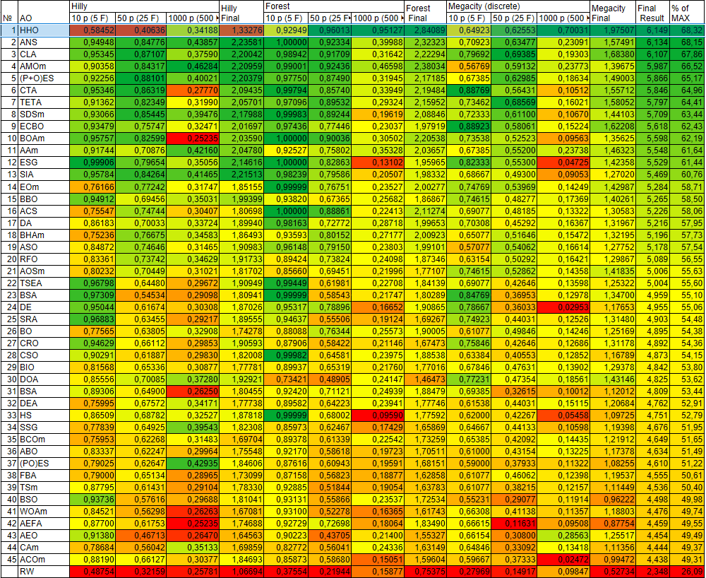
Figure 2. Color coding of algorithms for the corresponding tests
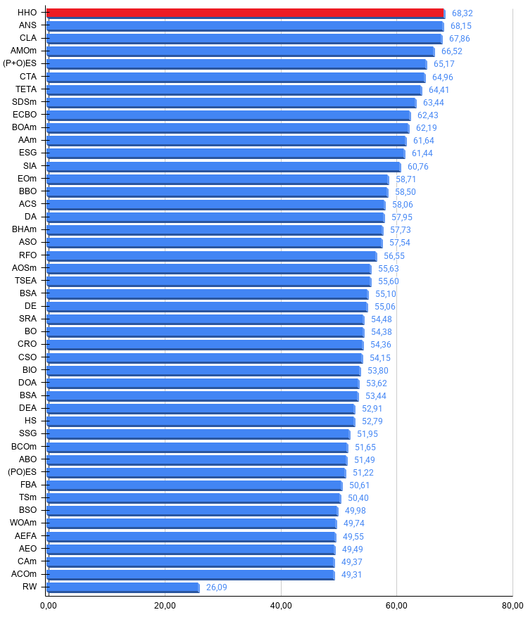
Figure 3. Histogram of results (0–100; higher is better; 100 is the theoretical maximum). The archive contains a script for calculating the ranking table.
Pros and Cons of the HHO Algorithm
Pros:
- Good performance on high-dimensional instances of the Forest function.
Cons:
- Weak convergence on the Hilly function.
- Computational complexity.
An archive containing the latest versions of the algorithm code is attached to the article. The author of this article does not assume responsibility for the absolute accuracy of the descriptions of canonical algorithms; changes have been made to many of them to improve their search capabilities. The conclusions and judgments presented in the articles are based on the results of the experiments conducted.
Programs used in the article
| # | Name | Type | Description |
|---|---|---|---|
| 1 | #C_AO.mqh | Include file | Parent class for population-based optimization algorithms |
| 2 | #C_AO_enum.mqh | Include file | Enumeration of population-based optimization algorithms |
| 3 | TestFunctions.mqh | Include file | Test function library |
| 4 | TestStandFunctions.mqh | Include file | Test bench function library |
| 5 | TestStand3D.mqh | Include file | 3D visualization panel for a test bench |
| 6 | Utilities.mqh | Include file | Utility functions library |
| 7 | CalculationTestResults.mqh | Include file | Script for calculating results for the comparison table |
| 8 | Testing AOs.mq5 | Script | Unified test bench for all population-based optimization algorithms |
| 9 | Simple use of population optimization algorithms.mq5 | Script | Simple example of using population-based optimization algorithms without visualization |
| 10 | Test_HHO.mq5 | Script | HHO test bench |
Translated from Russian by MetaQuotes Ltd.
Original article: https://www.mql5.com/ru/articles/21898
Warning: All rights to these materials are reserved by MetaQuotes Ltd. Copying or reprinting of these materials in whole or in part is prohibited.
This article was written by a user of the site and reflects their personal views. MetaQuotes Ltd is not responsible for the accuracy of the information presented, nor for any consequences resulting from the use of the solutions, strategies or recommendations described.

 Features of Custom Indicators Creation
 Ollivier-Ricci Curvature: Reading the Shape of a Correlation Network, Not Its Level
 Features of Experts Advisors
 Price Action Analysis Toolkit Development (Part 84): Validating Recorded Double-Bottom Samples

- Free trading apps
- Over 8,000 signals for copying
- Economic news for exploring financial markets
You agree to website policy and terms of use
What a great discovery!
I really appreciate this
Many thanks
What a great discovery!
I appreciate this
Many thanks