

The Dragonfly Algorithm (DA)
 87
87
 0
0

Table of Contents
Introduction
Let's consider another modern population-based metaheuristic method — the Dragonfly Algorithm — for our optimization problems. Dragonflies are among the most spectacular flying insects and have existed on the planet for nearly 300 million years. Their unique ability to maneuver in the air — hovering, instantaneous changes in direction, and flight in six degrees of freedom — has long attracted the attention of researchers. However, in the field of metaheuristic optimization, it is not the aerodynamics of an individual dragonfly that is of particular interest, but rather the collective behavior of swarms.
In 2015, Seyedali Mirjalili proposed the Dragonfly Algorithm (DA), which models two types of dragonfly swarm behavior: static and dynamic. A static swarm forms during hunting — dragonflies gather in small groups and move over a limited area in search of prey. A dynamic swarm forms during migration — large groups move in the same direction over considerable distances. These two modes naturally correspond to the two fundamental phases of optimization: exploitation (exploiting the solutions found) and exploration (exploring new search space).
Implementation of the Algorithm
Imagine a warm summer evening by a pond. Dozens of dragonflies are circling above the water. If you look closely, you can notice a pattern: dragonflies do not fly randomly. They stay together as a group but do not collide; they fly in roughly the same direction, but each follows its own path. If one of them finds a swarm of gnats, the others move in; if a bird appears, the whole group scatters. The algorithm simulates a swarm of dragonflies, where each dragonfly represents a potential solution to the problem, and the quality of the solution is the amount of prey caught.
Five Simple Rules of Behavior. Each dragonfly in the algorithm follows five rules. They are all intuitive because we observe similar behavior in everyday life — in crowds of people, in flocks of birds, and in traffic.
1. Do Not Crowd Others (Separation). If your neighbors get too close, move away. This rule prevents all the dragonflies from gathering at one point. For example, you are standing in an elevator with other people; no one has made any arrangements, but everyone has instinctively spread out around the elevator at roughly equal distances. In optimization terms: if all agents converge at a single point, the algorithm will stop exploring the space and get stuck. Separation protects against this.
2. Fly Like the Others (Alignment). Look where your neighbors are flying, and adjust your velocity and direction accordingly. This rule ensures coordinated movement of the group. Imagine that you are walking along a sidewalk in a flow of people: without even thinking about it, you walk at roughly the same speed and in the same direction as those around you. In optimization: if one dragonfly finds a promising direction, its neighbors begin moving in the same direction, intensifying the search in that area.
3. Stay with the Swarm (Cohesion). Aim for the center of the group of neighbors; do not fall behind or fly far away on your own. Imagine a group of tourists in an unfamiliar city: everyone wants to look around, but no one strays too far from the group — so they don't get lost. In optimization, cohesion prevents agents from scattering uncontrollably throughout the search space, keeping them together so they can explore promising areas collaboratively.
4. Fly toward the food (Food Attraction). If you find a food source nearby, move toward it. In the algorithm, “food” is the best solution found so far. For example, you are walking through a shopping mall and smell the aroma of freshly baked goods. Your feet naturally carry you in that direction, so in optimization, the best solution found draws the agents toward it, concentrating the search around the most promising point.
5. Run from the enemy (Enemy Distraction). If you spot a predator nearby, get away from it. The danger is the worst solution found. If you are walking down an unfamiliar side street in the city and see a warning sign, you will turn around and take a different route. Repulsion from the worst solutions helps avoid wasting time on unpromising areas of the search space.
How these rules work together. At each step of the algorithm, each dragonfly calculates all five factors and combines them into a single movement vector: it must move away from its neighbors (separation), fly in the direction they are flying (alignment), but not break away from the group (cohesion), while staying on course toward the food (food) and away from the predator (enemy). The resulting direction is a compromise between all five tendencies. Inertia also comes into play — a dragonfly cannot change direction instantly, so part of its previous velocity is retained.
Here's a simple numerical example. Suppose a dragonfly is located at point X = 5 along one coordinate. The five factors yield the following values:
- Separation = +2 (neighbors are on the left, so it needs to move to the right)
- Alignment = −1 (neighbors tend to fly to the left on average)
- Cohesion = −3 (the center of the flock is to the left)
- Food = +4 (the best solution is to the right)
- Enemy = +1 (the worst solution is to the left; we move to the right)
With weights s = 0.05, a = 0.05, c = 0.05, f = 1.2, e = 0.05, and inertia w·ΔX = 0.3: ΔX = 0.05·2 + 0.05·(−1) + 0.05·(−3) + 1.2·4 + 0.05·1 + 0.3 = 5.15. New position: X = 5 + 5.15 = 10.15. The dragonfly has shifted significantly to the right — mainly because of food attraction (4 × 1.2 = 4.8), which dominates. The other factors made only minimal corrections.
A lone dragonfly and Lévy flight. Sometimes a dragonfly finds itself isolated — it has no neighbors within its viewing radius, and the food is far away, too. In this case, the five rules are useless: there is no one to repel itself from, no one to join, and nothing to pursue. What does a lone dragonfly do? It performs a Lévy flight — a special type of random walk named after the French mathematician Paul Lévy. How is it different from a regular random search? An ordinary random step is like flipping a coin: a step forward or backward by the same distance. A Lévy flight is a series of small steps punctuated by occasional big leaps.
How the algorithm matures. The algorithm has one key feature: its behavior changes over time. At the beginning, dragonflies behave like explorers. By the end — like a group of hunters who have already found their target and are closing in. This is achieved through three adaptive parameters:
The vision radius (r) is small at first. Dragonflies see few neighbors, often find themselves isolated, and perform Lévy flights, exploring the entire space. Toward the end, the radius grows to enormous values: all the dragonflies can see one another and act as a single organism, precisely adjusting their positions. The weight coefficients (s, a, c, e) decrease from nonzero values to zero during the first half of the iterations. In the second half, only food attraction (f) remains.
Inertia (w) decreases from 0.9 to 0.4. High initial inertia means that the dragonfly takes a long time to pick up speed and cannot turn quickly; this helps it explore over long distances. Low inertia toward the end allows for precise maneuvers near the optimum.
In summary: one step of the algorithm. Let's put it all together. At each iteration, the algorithm performs the following:
For each dragonfly:
- Look around — find neighbors within radius r.
- Calculate the five factors: separation, alignment, cohesion, food, and enemy.
- If there is food nearby and enough neighbors, perform a full update by combining all five factors with adaptive weights.
- If there is no food nearby but there are neighbors — move according to the swarm rules (separation + alignment + cohesion).
- If you are isolated, perform a Lévy flight.
Constrain the position to the boundaries of the search space. After all the dragonflies have moved:
- Calculate the fitness of each solution.
- Update "food" (the best solution) and "enemy" (the worst solution).
Repeat until all iterations have been completed. The best solution found over all iterations is the result of the algorithm.
Let's review once again the behavior of each dragonfly in the swarm:
- Separation — dragonflies avoid collisions with their neighbors by veering away from individuals that are too close. In terms of optimization, this prevents agents from clustering at a single point and maintains population diversity.
- Alignment — dragonflies coordinate their velocity and flight direction with their neighbors. This ensures coordinated movement of the group in promising directions.
- Cohesion — dragonflies are drawn toward the center of mass of their neighbors. This mechanism draws scattered agents back toward the group, preventing them from flying off uncontrollably.
- Food attraction — dragonflies move toward a food source, which corresponds to agents being attracted to the best solution found.
- Enemy distraction — dragonflies move away from predators, which in the model means repulsion from the worst known solution.
Mathematical model. For each dragonfly i with position X and velocity vector DeltaX, five corrective vectors are calculated based on neighbors within radius r:
Separation (Eq. 1): S = -SUM(X - Xj)
Alignment (Eq. 2): A = SUM(Vj) / N
Cohesion (Eq. 3): C = SUM(Xj) / N - X
Food (Eq. 4): F = X+ - X
Enemy (Eq. 5): E = X- + X; where N is the number of neighbors, Vj is the velocity of the j-th neighbor, X+ is the position of the best solution (Food), and X- is the position of the worst solution (Enemy).
The velocity vector update combines all five factors with adaptive weights (Eq. 6):
DeltaX(t+1) = s*S + a*A + c*C + f*F + e*E + w*DeltaX(t), and the new position is calculated as (Eq. 7):
X(t+1) = X(t) + DeltaX(t+1)
When a dragonfly is isolated (with fewer than two neighbors within radius r and Food out of reach), it performs a random Lévy flight (Eq. 8) — a random walk with heavy tails, allowing both small steps and rare large jumps:
X(t+1) = X(t) + Levy(d) * X(t)
The Lévy step is calculated using the Mantegna algorithm (Eq. 9):
Levy = 0.01 * (r1 * sigma) / |r2|^(1/beta)
where r1 ~ N(0, sigma^2), r2 ~ N(0, 1), beta = 1.5, and sigma is defined via the Gamma function (Eq. 10).
Adaptive mechanism. A key feature of DA is the smooth transition from "exploration" to "exploitation" through adaptive parameters:
The neighborhood radius r increases with each iteration. At the start of optimization, dragonflies see few neighbors and therefore perform Lévy flights more often (exploration). By the end, the radius covers most of the space, and all agents coordinate as a single swarm (exploitation).
The weighting coefficients (s, a, c, e) decrease from their maximum values to zero during the first half of the iterations. In the second half, only food attraction (f) remains, which concentrates the search around the best solution.
The inertia "w" decreases from 0.9 to 0.4, gradually reducing the influence of the previous velocity and enabling fine-tuning of the position at the end of the optimization. This mechanism does not require any user configuration — the only external parameter of the algorithm is the population size.
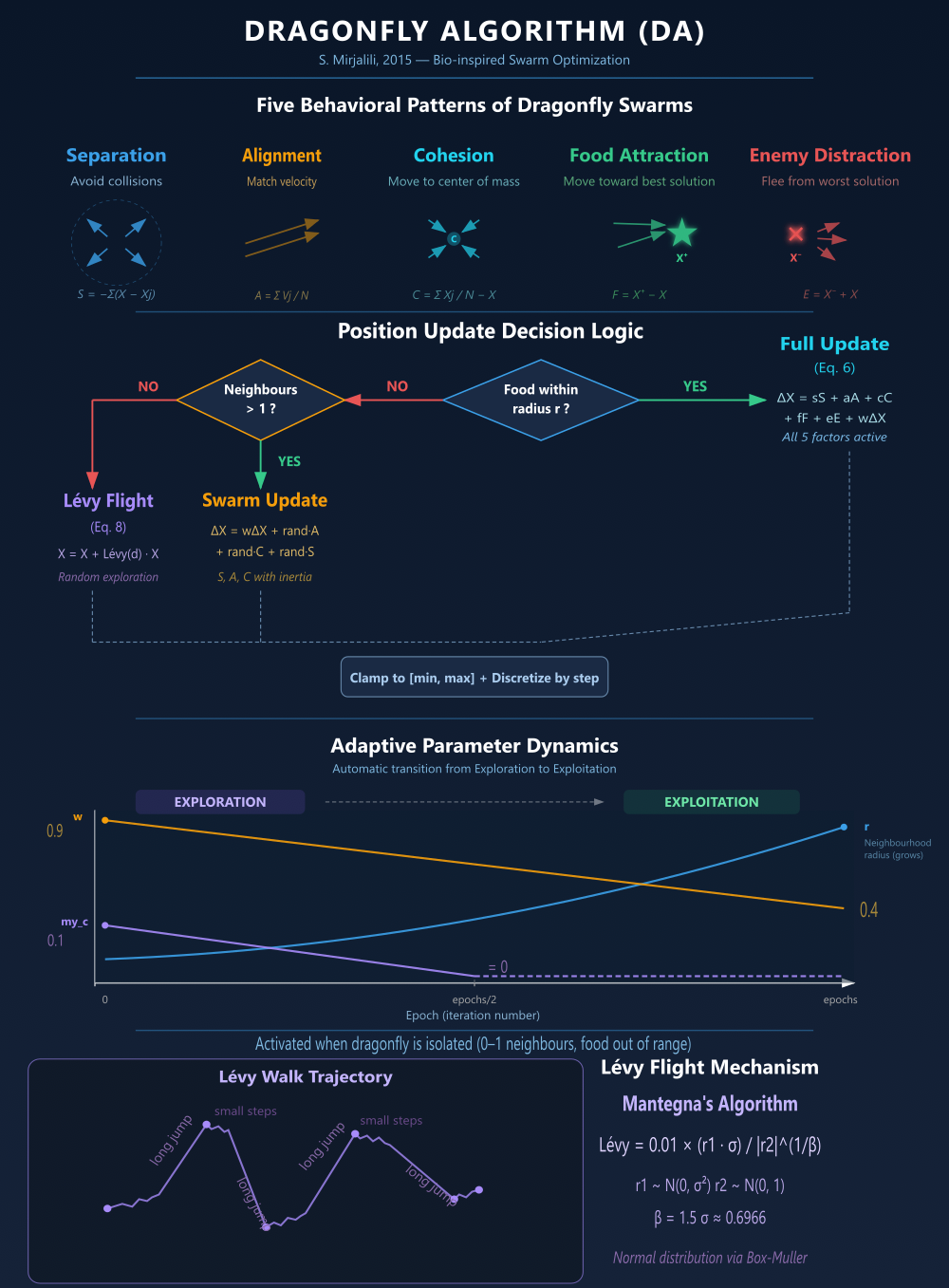
The illustration consists of four sections:
1. Five Behavioral Patterns — visual diagrams of all five factors (Separation, Alignment, Cohesion, Food, Enemy) featuring dragonfly icons, directional arrows, and formulas.
2. Position Update Decision Logic — flowchart for selecting the movement mode: Food within the radius → Full Update (Eq. 6); otherwise, check whether the number of neighbors is > 1 → Swarm Update or Lévy Flight (Eq. 8). All three paths converge at the final Clamp + Discretize stage.
3. Adaptive Parameter Dynamics — graphs of three key parameters over time: r (increasing), w (decreasing from 0.9 to 0.4), and my_c (decreasing from 0.1 to 0 during the first half). The transition from Exploration to Exploitation is shown.
4. Lévy Flight Mechanism — a visualization of the Lévy flight trajectory (many small steps + occasional long jumps) and the Mantegna formula with parameters.
We can now move directly on to the algorithm implementation.
The C_AO_DA_Dragonfly class implements the Dragonfly Algorithm, which is inspired by the swarming behavior of dragonflies in nature. The class inherits from the base class "C_AO," which provides a common infrastructure for all population-based optimization algorithms: an array of agents, search space boundaries, storage for the best and worst solutions found, and utilities for generating random numbers and discretizing coordinates.
The class stores the velocities of all agents in a flat array called "DeltaX", with each agent corresponding to a set of velocity components across all coordinates. Access to the elements of this array is provided through the helper methods "GetDX" and "SetDX", which calculate the linear index based on the agent index and the coordinate index.
The algorithm operates on two key points in the search space: "Food" and "Enemy". The former stores the position and fitness of the best solution found so far and acts as an attractor — agents that are close enough to "Food" are drawn toward this point. "Enemy" stores the position and fitness of the worst solution found and acts as a repellent — agents near "Enemy" are repelled from it.
To manage the adaptive parameters, the class maintains the total number of optimization epochs and a counter for the current epoch. The ratio between them determines the values of the neighborhood radius, inertia, and weighting coefficients at each step. The range width for each coordinate and the maximum allowable velocity — equal to one-hundredth of that range width — are also precomputed. The only externally configurable parameter is the population size. All other coefficients in the algorithm are calculated automatically.
The "SetParams" method reads the population size value from the external "params" array and writes it to the class's internal field. It is called after the test script has written the required parameter values. This algorithm has only one parameter, so the method is trivial, but its presence ensures a consistent interface with all other algorithms.
//————————————————————————————————————————————————————————————————————
class C_AO_DA_Dragonfly : public C_AO
{
  public: //----------------------------------------------------------
  ~C_AO_DA_Dragonfly () { }
  C_AO_DA_Dragonfly ()
  {
    ao_name = "DA(Dragonfly)";
    ao_desc = "Dragonfly Algorithm";
    ao_link = "https://www.mql5.com/en/articles/21310";

    popSize = 50;

    ArrayResize (params, 1);
    params [0].name = "popSize"; params [0].val = popSize;
  }

  void SetParams ()
  {
    popSize = (int)params [0].val;
  }

  bool Init (const double &rangeMinP  [],
             const double &rangeMaxP  [],
             const double &rangeStepP [],
             const int     epochsP = 0);

  void Moving   ();
  void Revision ();

  private: //---------------------------------------------------------

  // Velocities (DeltaX)
  double DeltaX [];  // [popSize * coords] flat array

  // Food (best) and Enemy (worst)
  double Food_pos [];
  double Food_f;
  double Enemy_pos [];
  double Enemy_f;

  // Iteration tracking
  int    epochs;
  int    epochNow;

  // Helpers
  double Delta_max [];  // max velocity per dimension
  double r_base    [];  // (ub-lb) per dimension

  double LevyStep ();
  double RandN    ();   // normal distribution N(0,1) generated by the Box-Muller method

  // Flat array access helpers
  double GetDX  (int i, int c) { return DeltaX  [i * coords + c]; }
  void   SetDX  (int i, int c, double v) { DeltaX [i * coords + c] = v; }
};
//————————————————————————————————————————————————————————————————————
The Init method performs full initialization of the algorithm before the optimization loop starts. It accepts arrays of the lower and upper bounds of the search space, the discretization steps for each coordinate, and the total number of epochs.
First, the parent class's "StandardInit" method is called; it resets the random number generator, sets the fitness of the best solution to negative infinity, and allocates memory for the arrays of agents, bounds, and best coordinates. If an error occurs, initialization is aborted. Next, the total number of epochs is saved — it is needed to calculate the adaptive parameters in "Moving". If the value passed is zero or negative, the default value — one thousand — is used. The current epoch counter is reset.
Memory is allocated for a flat array of velocities. For each coordinate, the range width — the difference between the upper and lower bound — is precomputed, along with the maximum allowable velocity, which is equal to one-hundredth of that width. The velocity limit prevents excessively large movements in a single step.
The "Food" position is initialized with a fitness of negative infinity, and the "Enemy" position is initialized with a fitness of positive infinity. This ensures that the first agent to be evaluated will update both positions. The initial positions of all agents are generated uniformly at random within the specified bounds and then discretized according to the step size. Initial velocities are also generated randomly within the same ranges.
//————————————————————————————————————————————————————————————————————
bool C_AO_DA_Dragonfly::Init (const double &rangeMinP  [],
                              const double &rangeMaxP  [],
                              const double &rangeStepP [],
                              const int     epochsP = 0)
{
  if (!StandardInit (rangeMinP, rangeMaxP, rangeStepP)) return false;

  //------------------------------------------------------------------
  epochs   = epochsP > 0 ? epochsP : 1000;
  epochNow = 0;

  //--- allocate DeltaX
  ArrayResize (DeltaX, popSize * coords);

  //--- Delta_max and r_base
  ArrayResize (Delta_max, coords);
  ArrayResize (r_base,    coords);
  for (int c = 0; c < coords; c++)
  {
    r_base    [c] = rangeMax [c] - rangeMin [c];
    Delta_max [c] = r_base [c] / 100.0;
  }

  //--- Food (best) and Enemy (worst) — for maximization
  ArrayResize (Food_pos,  coords);
  ArrayResize (Enemy_pos, coords);
  Food_f  = -DBL_MAX;
  Enemy_f =  DBL_MAX;

  //--- Initialize positions randomly, DeltaX randomly
  for (int i = 0; i < popSize; i++)
  {
    for (int c = 0; c < coords; c++)
    {
      a [i].c [c] = u.RNDfromCI (rangeMin [c], rangeMax [c]);
      a [i].c [c] = u.SeInDiSp  (a [i].c [c], rangeMin [c], rangeMax [c], rangeStep [c]);

      SetDX (i, c, u.RNDfromCI (rangeMin [c], rangeMax [c]));
    }
  }

  return true;
}
//————————————————————————————————————————————————————————————————————
The Moving method is the central part of the algorithm, performing the movement of all agents in the current epoch. It is called once per iteration before the fitness function is computed. After it is executed, the external code calculates the fitness values for each agent and passes control to the "Revision" method.
At the beginning of the method, the epoch counter is incremented, and the adaptive parameters that control the balance between exploration of the search space and exploitation of the solutions found are calculated.
The adaptive neighborhood radius is calculated for each coordinate as one-quarter of the range width plus twice that width multiplied by the fraction of elapsed epochs. At the beginning of the optimization process, the radius is small — agents see few neighbors, are often isolated, and perform Lévy flights, exploring the entire space. By the end of the optimization process, the radius grows so large that it encompasses virtually the entire search space — all agents can see one another and act as a coordinated swarm, fine-tuning their positions near the optimum.
Inertia decreases linearly from 0.9 to 0.4 throughout all epochs. High initial inertia means that the agent retains a significant portion of its previous velocity and moves in long jumps, which helps it quickly cover large distances. Low inertia toward the end allows for short, precise movements to fine-tune the position.
The "my_c" coefficient decreases linearly from 0.1 to zero during the first half of the epochs and remains zero during the second half; it scales the weights of separation, alignment, cohesion, and enemy repulsion. When "my_c" reaches zero, all these weights are reset to zero, and the agents are driven solely by food attraction toward the best solution — the algorithm switches entirely to exploitation.
The weight coefficients for the five behavioral factors are calculated once per epoch. The separation, alignment, and cohesion coefficients are equal to the product of 2, a random number between zero and one, and "my_c". The enemy repulsion coefficient is simply "my_c". The food attraction coefficient is equal to the product of 2 and a random number — it does not depend on "my_c" and remains active throughout the entire optimization process.
Next, a five-step procedure is performed for each agent. In the first step, the neighbors of the current agent are identified. For each other agent, the system checks whether the distance to that agent does not exceed the adaptive radius along each coordinate. An agent is considered a neighbor only if the distance along all coordinates simultaneously falls within the corresponding components of the radius. In parallel with counting the number of neighbors, three sets of sums are accumulated: the sums of the neighbors' velocities, the sums of their positions, and the sums of the differences between the neighbors' positions and the current agent's position. These sums are used to calculate the behavioral factors without iterating through the array again.
In the second step, five behavioral factors are calculated. Separation is equal to the negative sum of the differences between the positions of the neighbors and the current agent — this forms a vector directed away from the cluster of neighbors, preventing collisions. In this implementation, separation is enabled when there are more than four neighbors; otherwise, it is set to zero. Alignment is equal to the average velocity of all neighbors and causes the agent to fly in the same direction as the rest of the group; if there are fewer than two neighbors, the agent's own velocity is used. Cohesion is equal to the difference between the average position of the neighbors and the agent's current position — this is a vector pointing toward the group's center of mass; if there are too few neighbors, it is set to zero.
Food attraction is equal to the difference between the "Food" position and the agent's position, but it is calculated only if "Food" is within the adaptive radius in all coordinates; otherwise, it is set to zero. Enemy repulsion is calculated as the sum of the "Enemy" position and the agent's position, and is also activated only when "Enemy" is within the radius.
In the third step, boundary wrap-around is performed with a velocity reset. If an agent's position along any coordinate exceeds the upper boundary, it is moved to the lower boundary, and vice versa. During this wrap-around, the corresponding velocity component is reset to a random value between zero and one.
In the fourth step, the agent's velocity and position are updated. The update mode is determined by two conditions: whether "Food" is within the adaptive radius and whether the agent has more than one neighbor. If "Food" is within the radius, a full update is performed: the new velocity is equal to the weighted sum of all five factors plus the inertia component of the previous velocity. This is the algorithm's core formula, which combines all behavioral signals into a single resulting movement.
If "Food" is outside the radius but the agent has more than one neighbor, a swarm update is performed without explicit food attraction: the velocity is formed from inertia and randomly weighted alignment, cohesion, and separation factors. The agent coordinates with the nearest group until it is close enough to "Food." If "Food" is outside the radius and the agent has no more than one neighbor, the agent performs a Lévy flight: the new position is equal to the current position plus the product of the Lévy step and the current position, and the velocity is reset to zero. This mode provides stochastic exploration of the space when the agent is isolated from the swarm.
In all three modes, the velocity is limited in absolute value by "Delta_max" for each coordinate, preventing excessively large displacements.
In the fifth step, the position is strictly constrained by the boundaries of the search space — values exceeding the maximum are clipped to the maximum, and values below the minimum are clipped to the minimum — and is discretized using the step via the "SeInDiSp" method, providing a final guarantee of coordinate validity before the fitness function is calculated.
//————————————————————————————————————————————————————————————————————
void C_AO_DA_Dragonfly::Moving ()
{
  epochNow++;

  double iter_ratio = (double)epochNow / (double)epochs;

  //--- Adaptive neighborhood radius: r = (ub - lb)/4 + (ub - lb) * (iter / Max_iter) * 2
  double r [];
  ArrayResize (r, coords);
  for (int c = 0; c < coords; c++)
  {
    r [c] = r_base [c] / 4.0 + r_base [c] * iter_ratio * 2.0;
  }

  //--- Inertia weight: w = 0.9 - iter*((0.9-0.4)/Max_iter)
  double w = 0.9 - epochNow * ((0.9 - 0.4) / (double)epochs);

  //--- Adaptive coefficient my_c = 0.1 - iter*(0.1/(Max_iter/2))
  double my_c = 0.1 - epochNow * (0.1 / ((double)epochs / 2.0));
  if (my_c < 0.0) my_c = 0.0;

  //--- Weights (computed once per epoch, as in MATLAB)
  double s_w = 2.0 * u.RNDfromCI (0.0, 1.0) * my_c; // Separation weight
  double a_w = 2.0 * u.RNDfromCI (0.0, 1.0) * my_c; // Alignment weight
  double c_w = 2.0 * u.RNDfromCI (0.0, 1.0) * my_c; // Cohesion weight
  double f_w = 2.0 * u.RNDfromCI (0.0, 1.0);        // Food attraction weight
  double e_w = my_c;                                // Enemy distraction weight

  //--- For each dragonfly
  for (int i = 0; i < popSize; i++)
  {
    //================================================================
    // 1. Find neighbors within a radius of r
    //================================================================
    int nCount = 0;

    double sumNDX [];  ArrayResize (sumNDX, coords);  ArrayInitialize (sumNDX, 0.0);
    double sumNX  [];  ArrayResize (sumNX,  coords);  ArrayInitialize (sumNX,  0.0);
    double sepV   [];  ArrayResize (sepV,   coords);  ArrayInitialize (sepV,   0.0);

    for (int j = 0; j < popSize; j++)
    {
      if (j == i) continue;

      // Per-dimension distance check: all (dist <= r)
      bool inNeighbour = true;
      for (int c = 0; c < coords; c++)
      {
        if (MathAbs (a [i].c [c] - a [j].c [c]) > r [c])
        {
          inNeighbour = false;
          break;
        }
      }

      if (inNeighbour)
      {
        nCount++;
        for (int c = 0; c < coords; c++)
        {
          sumNDX [c] += GetDX (j, c);
          sumNX  [c] += a [j].c [c];
          sepV   [c] += (a [j].c [c] - a [i].c [c]);
        }
      }
    }

    //================================================================
    // 2. Compute swarm behaviors (Eq. 3.1–3.5)
    //================================================================

    //--- Separation S (Eq. 3.1): S = -Σ(Xj - Xi)
    //    requires neighbors_no > 1
    double S [];  ArrayResize (S, coords);
    if (nCount > 4)
    {
      for (int c = 0; c < coords; c++) S [c] = -sepV [c];
    }
    else
    {
      ArrayInitialize (S, 0.0);
    }

    //--- Alignment A (Eq. 3.2): A = Σ Vj / N
    //    If there are no neighbors: A = own DeltaX
    double A [];  ArrayResize (A, coords);
    if (nCount > 1)
    {
      for (int c = 0; c < coords; c++) A [c] = sumNDX [c] / (double)nCount;
    }
    else
    {
      for (int c = 0; c < coords; c++) A [c] = GetDX (i, c);
    }

    //--- Cohesion C (Eq. 3.3): C = Σ Xj / N - Xi
    //    If there are no neighbors: C = 0
    double C [];  ArrayResize (C, coords);
    if (nCount > 1)
    {
      for (int c = 0; c < coords; c++) C [c] = sumNX [c] / (double)nCount - a [i].c [c];
    }
    else
    {
      for (int c = 0; c < coords; c++) C [c] = 0.0;
    }

    //--- Food attraction F (Eq. 3.4): F = Food_pos - Xi (if food is within r)
    double F [];  ArrayResize (F, coords);  ArrayInitialize (F, 0.0);
    bool foodInRange = false;
    if (Food_f > -DBL_MAX)
    {
      foodInRange = true;
      for (int c = 0; c < coords; c++)
      {
        if (MathAbs (a [i].c [c] - Food_pos [c]) > r [c])
        {
          foodInRange = false;
          break;
        }
      }
      if (foodInRange)
      {
        for (int c = 0; c < coords; c++) F [c] = Food_pos [c] - a [i].c [c];
      }
    }

    //--- Enemy distraction E (Eq. 3.5)
    //    Enemy = Enemy_pos + Xi (if enemy is within r)
    double E [];  ArrayResize (E, coords);  ArrayInitialize (E, 0.0);
    if (Enemy_f < DBL_MAX)
    {
      bool enemyInRange = true;
      for (int c = 0; c < coords; c++)
      {
        if (MathAbs (a [i].c [c] - Enemy_pos [c]) > r [c])
        {
          enemyInRange = false;
          break;
        }
      }
      if (enemyInRange)
      {
        for (int c = 0; c < coords; c++) E [c] = Enemy_pos [c] + a [i].c [c];
      }
    }

    //================================================================
    // 3. Boundary wrap-around with velocity reset
    //    AFTER S/A/C/F/E computation, BEFORE velocity/position update
    //================================================================
    for (int c = 0; c < coords; c++)
    {
      if (a [i].c [c] > rangeMax [c])
      {
        a [i].c [c] = rangeMin [c];
        SetDX (i, c, u.RNDfromCI (0.0, 1.0));
      }
      if (a [i].c [c] < rangeMin [c])
      {
        a [i].c [c] = rangeMax [c];
        SetDX (i, c, u.RNDfromCI (0.0, 1.0));
      }
    }

    //================================================================
    // 4. Update velocity and position
    //================================================================
    if (!foodInRange)
    {
      // Food NOT in range
      if (nCount > 1) // neighbours_no > 1
      {
        // Swarm behavior: use S, A, and C with inertia
        for (int c = 0; c < coords; c++)
        {
          double dx = w * GetDX (i, c)
                      + u.RNDfromCI (0.0, 1.0) * A [c]
                      + u.RNDfromCI (0.0, 1.0) * C [c]
                      + u.RNDfromCI (0.0, 1.0) * S [c];

          if (dx >  Delta_max [c]) dx =  Delta_max [c];
          if (dx < -Delta_max [c]) dx = -Delta_max [c];

          SetDX (i, c, dx);
          a [i].c [c] += dx;
        }
      }
      else
      {
        // Lévy flight (Eq. 3.8): X = X + Levy(d) * X
        for (int c = 0; c < coords; c++)
        {
          a [i].c [c] += LevyStep () * a [i].c [c];
          SetDX (i, c, 0.0);
        }
      }
    }
    else
    {
      // Food IS in range — full update (Eq. 3.6)
      // ΔX(t+1) = (s·S + a·A + c·C + f·F + e·E) + w·ΔX(t)
      for (int c = 0; c < coords; c++)
      {
        double dx = (s_w * S [c] + a_w * A [c] + c_w * C [c] + f_w * F [c] + e_w * E [c])
                    + w * GetDX (i, c);

        if (dx >  Delta_max [c]) dx =  Delta_max [c];
        if (dx < -Delta_max [c]) dx = -Delta_max [c];

        SetDX (i, c, dx);
        a [i].c [c] += dx;
      }
    }

    //================================================================
    // 5. Post-update clamp to bounds and discretize
    //    X = X.*(~(Flag4ub+Flag4lb)) + ub.*Flag4ub + lb.*Flag4lb
    //================================================================
    for (int c = 0; c < coords; c++)
    {
      if (a [i].c [c] > rangeMax [c]) a [i].c [c] = rangeMax [c];
      if (a [i].c [c] < rangeMin [c]) a [i].c [c] = rangeMin [c];
      a [i].c [c] = u.SeInDiSp (a [i].c [c], rangeMin [c], rangeMax [c], rangeStep [c]);
    }
  }
}
//————————————————————————————————————————————————————————————————————
The Revision method revises the results after the external code has calculated the fitness values for all agents. It is called once per epoch and iterates over the entire population, performing three updates.
The first update concerns the global best solution. If the current agent's fitness exceeds the fitness of the best solution "fB" in the parent class, the new fitness is recorded and the coordinates are copied to the array "cB". These fields are used by the test bench to track optimization progress and perform a final quality assessment.
The second update concerns the internal "Food" attractor. If an agent's fitness exceeds the current "Food_f", the fitness and position of "Food" are updated. Although "Food" and "fB" in practice contain the same value, they are logically separate: "fB" and "cB" are the interface to the outside world, while "Food" is the algorithm's internal mechanics, used in "Moving" to calculate the attraction vector.
The third update concerns the internal repellent "Enemy". Before the update, the system checks whether the agent is within the boundaries of the search space in all coordinates. If an agent is within the boundaries and its fitness is lower than the current "Enemy_f", the fitness and position of "Enemy" are updated. Boundary checking prevents "Enemy" from being assigned to invalid points that could generate incorrect repulsion vectors.
//————————————————————————————————————————————————————————————————————
void C_AO_DA_Dragonfly::Revision ()
{
  for (int i = 0; i < popSize; i++)
  {
    //--- Update global best (Food in maximization)
    if (a [i].f > fB)
    {
      fB = a [i].f;
      ArrayCopy (cB, a [i].c, 0, 0, coords);
    }

    if (a [i].f > Food_f)
    {
      Food_f = a [i].f;
      ArrayCopy (Food_pos, a [i].c, 0, 0, coords);
    }

    //--- Update global worst (Enemy in maximization)
    // Only if within bounds
    bool inBounds = true;
    for (int c = 0; c < coords; c++)
    {
      if (a [i].c [c] > rangeMax [c] || a [i].c [c] < rangeMin [c])
      {
        inBounds = false;
        break;
      }
    }

    if (inBounds && a [i].f < Enemy_f)
    {
      Enemy_f = a [i].f;
      ArrayCopy (Enemy_pos, a [i].c, 0, 0, coords);
    }
  }
}
//————————————————————————————————————————————————————————————————————
The RandN method generates random numbers with a normal distribution N(0, 1) using the Box–Muller transform. Two independent uniformly distributed numbers are taken from the interval from zero to one, and one normally distributed value is computed from them: the square root of minus two times the natural logarithm of the first number, multiplied by the cosine of the product of 2π and the second number.
This method is necessary for the correct implementation of Lévy flight. In Mantegna's formula, the variables "r1" and "r2" must be normally distributed. Using a uniform distribution instead of a normal distribution distorts the heavy-tailed nature of the Lévy distribution: the probability of long jumps decreases, which reduces the efficiency of space exploration and essentially turns a Lévy flight into an ordinary random walk.
To prevent calculation of the logarithm of zero, the first uniform number is bounded below by a small value.
//————————————————————————————————————————————————————————————————————
// Normal distribution N(0,1) via the Box–Muller transform
double C_AO_DA_Dragonfly::RandN ()
{
  double u1 = u.RNDfromCI (0.0, 1.0);
  double u2 = u.RNDfromCI (0.0, 1.0);

  // Avoid log(0)
  if (u1 < 1e-10) u1 = 1e-10;

  return MathSqrt (-2.0 * MathLog (u1)) * MathCos (2.0 * M_PI * u2);
}
//————————————————————————————————————————————————————————————————————
The LevyStep method computes a single scalar Lévy step of a Lévy flight using Mantegna's algorithm. A Lévy flight is a random walk in which step lengths follow a power-law distribution: the vast majority of steps are small, but very long jumps occur occasionally. This type of random walk has been mathematically proven to be optimal for finding sparsely distributed targets and is used in many metaheuristic algorithms during the space exploration phase.
The step is calculated as the product of a scaling factor of 0.01 and a quotient: the numerator is a normally distributed value multiplied by the precomputed constant "sigma", and the denominator is the absolute value of another normally distributed value raised to the power of the reciprocal of the stability parameter "beta".
The constant "sigma" is precomputed using a formula involving the Gamma function for "beta" equal to 1.5 and is approximately 0.6966. The multiplier 0.01 provides a moderate step amplitude, preventing excessively large outliers. The denominator is protected against division by zero by being bounded below by a small value.
The returned scalar step is used in the "Moving" method: it is multiplied by the agent's current position and added to it, forming a new position during a Lévy flight.
//————————————————————————————————————————————————————————————————————
// Lévy flight step — Mantegna's algorithm (Eq. 9, 10)
// Levy(x) = 0.01 * (r1 * sigma) / |r2|^(1/beta)
// where r1 ~ N(0, sigma^2), r2 ~ N(0, 1), beta = 1.5
// sigma = (Gamma(1+beta)*sin(pi*beta/2) / (Gamma((1+beta)/2)*beta*2^((beta-1)/2)))^(1/beta)
double C_AO_DA_Dragonfly::LevyStep ()
{
  double beta = 1.5;

  // For beta = 1.5:
  // Gamma(2.5)   = 1.329340
  // sin(3*pi/4)  = 0.707107
  // Gamma(1.25)  = 0.906402
  // 1.5 * 2^0.25 = 1.783811
  // sigma = (1.329340 * 0.707107 / 1.616873)^(1/1.5) ≈ 0.6966
  double sigma = 0.6966;

  double u_val = RandN () * sigma; // r1 ~ N(0, sigma^2)
  double v_val = MathAbs (RandN ());    // |r2|, r2 ~ N(0, 1)

  if (v_val < 1e-10) v_val = 1e-10;

  double step = u_val / MathPow (v_val, 1.0 / beta);

  return 0.01 * step;
}
//————————————————————————————————————————————————————————————————————
Test Results
The Dragonfly Algorithm (DA) achieved a score of 36% on our test bench, which, unfortunately, is not enough for it to qualify for the main ranking table. This is an average score, indicating that the algorithm has some difficulty solving optimization problems of varying complexity.=============================
5 Hilly's; Func runs: 10000; result: 0.6776724523765025
25 Hilly's; Func runs: 10000; result: 0.3961601008221486
500 Hilly's; Func runs: 10000; result: 0.27032293850032585
=============================
5 Forest's; Func runs: 10000; result: 0.6088666045448039
25 Forest's; Func runs: 10000; result: 0.3063399651091877
500 Forest's; Func runs: 10000; result: 0.18032255251950144
=============================
5 Megacity's; Func runs: 10000; result: 0.5061538461538462
25 Megacity's; Func runs: 10000; result: 0.21415384615384614
500 Megacity's; Func runs: 10000; result: 0.1035384615384625
=============================
All score: 3.26353 (36.26%)
Visualization of the Dragonfly Algorithm in operation on our test problems of varying dimensions and on standard functions.

DA_Dragonfly on the Hilly test function

DA_Dragonfly on the Forest test function

DA_Dragonfly on the Megacity test function

DA_Dragonfly on the standard Ackley function

DA_Dragonfly on the standard Paraboloid function
Based on the test results, the DA_Dragonfly algorithm is included in the ranking table for reference.
| No. | AO | Description | Hilly | Hilly Final | Forest | Forest Final | Megacity (discrete) | Megacity Final | Final Result | % of MAX | ||||||
| 10 p (5 F) | 50 p (25 F) | 1,000 p (500 F) | 10 p (5 F) | 50 p (25 F) | 1,000 p (500 F) | 10 p (5 F) | 50 p (25 F) | 1,000 p (500 F) | ||||||||
| 1 | ANS | across neighbourhood search | 0.94948 | 0.84776 | 0.43857 | 2.23581 | 1.00000 | 0.92334 | 0.39988 | 2.32323 | 0.70923 | 0.63477 | 0.23091 | 1.57491 | 6.134 | 68.15 |
| 2 | CLA | code lock algorithm (jo o) | 0.95345 | 0.87107 | 0.37590 | 2.20042 | 0.98942 | 0.91709 | 0.31642 | 2.22294 | 0.79692 | 0.69385 | 0.19303 | 1.68380 | 6.107 | 67.86 |
| 3 | AMOm | animal migration optimization M | 0.90358 | 0.84317 | 0.46284 | 2.20959 | 0.99001 | 0.92436 | 0.46598 | 2.38034 | 0.56769 | 0.59132 | 0.23773 | 1.39675 | 5.987 | 66.52 |
| 4 | (P+O)ES | (P+O) evolution strategies | 0.92256 | 0.88101 | 0.40021 | 2.20379 | 0.97750 | 0.87490 | 0.31945 | 2.17185 | 0.67385 | 0.62985 | 0.18634 | 1.49003 | 5.866 | 65.17 |
| 5 | CTA | comet tail algorithm (joo) | 0.95346 | 0.86319 | 0.27770 | 2.09435 | 0.99794 | 0.85740 | 0.33949 | 2.19484 | 0.88769 | 0.56431 | 0.10512 | 1.55712 | 5.846 | 64.96 |
| 6 | TETA | time evolution travel algorithm (joo) | 0.91362 | 0.82349 | 0.31990 | 2.05701 | 0.97096 | 0.89532 | 0.29324 | 2.15952 | 0.73462 | 0.68569 | 0.16021 | 1.58052 | 5.797 | 64.41 |
| 7 | SDSm | stochastic diffusion search M | 0.93066 | 0.85445 | 0.39476 | 2.17988 | 0.99983 | 0.89244 | 0.19619 | 2.08846 | 0.72333 | 0.61100 | 0.10670 | 1.44103 | 5.709 | 63.44 |
| 8 | ECBO | enhanced_colliding_bodies_optimization | 0.93479 | 0.75747 | 0.32471 | 2.01697 | 0.97436 | 0.77446 | 0.23037 | 1.97919 | 0.88923 | 0.58061 | 0.15224 | 1.62208 | 5.618 | 62.43 |
| 9 | BOAm | billiards optimization algorithm M | 0.95757 | 0.82599 | 0.25235 | 2.03590 | 1.00000 | 0.90036 | 0.30502 | 2.20538 | 0.73538 | 0.52523 | 0.09563 | 1.35625 | 5.598 | 62.19 |
| 10 | AAm | archery algorithm M | 0.91744 | 0.70876 | 0.42160 | 2.04780 | 0.92527 | 0.75802 | 0.35328 | 2.03657 | 0.67385 | 0.55200 | 0.23738 | 1.46323 | 5.548 | 61.64 |
| 11 | ESG | evolution of social groups (joo) | 0.99906 | 0.79654 | 0.35056 | 2.14616 | 1.00000 | 0.82863 | 0.13102 | 1.95965 | 0.82333 | 0.55300 | 0.04725 | 1.42358 | 5.529 | 61.44 |
| 12 | SIA | simulated isotropic annealing (joo) | 0.95784 | 0.84264 | 0.41465 | 2.21513 | 0.98239 | 0.79586 | 0.20507 | 1.98332 | 0.68667 | 0.49300 | 0.09053 | 1.27020 | 5.469 | 60.76 |
| 13 | EOm | extremal_optimization_M | 0.76166 | 0.77242 | 0.31747 | 1.85155 | 0.99999 | 0.76751 | 0.23527 | 2.00277 | 0.74769 | 0.53969 | 0.14249 | 1.42987 | 5.284 | 58.71 |
| 14 | BBO | biogeography-based optimization | 0.94912 | 0.69456 | 0.35031 | 1.99399 | 0.93820 | 0.67365 | 0.25682 | 1.86867 | 0.74615 | 0.48277 | 0.17369 | 1.40261 | 5.265 | 58.50 |
| 15 | ACS | artificial cooperative search | 0.75547 | 0.74744 | 0.30407 | 1.80698 | 1.00000 | 0.88861 | 0.22413 | 2.11274 | 0.69077 | 0.48185 | 0.13322 | 1.30583 | 5.226 | 58.06 |
| 16 | DA | dialectical algorithm | 0.86183 | 0.70033 | 0.33724 | 1.89940 | 0.98163 | 0.72772 | 0.28718 | 1.99653 | 0.70308 | 0.45292 | 0.16367 | 1.31967 | 5.216 | 57.95 |
| 17 | BHAm | black hole algorithm M | 0.75236 | 0.76675 | 0.34583 | 1.86493 | 0.93593 | 0.80152 | 0.27177 | 2.00923 | 0.65077 | 0.51646 | 0.15472 | 1.32195 | 5.196 | 57.73 |
| 18 | ASO | anarchy society optimization | 0.84872 | 0.74646 | 0.31465 | 1.90983 | 0.96148 | 0.79150 | 0.23803 | 1.99101 | 0.57077 | 0.54062 | 0.16614 | 1.27752 | 5.178 | 57.54 |
| 19 | RFO | royal flush optimization (joo) | 0.83361 | 0.73742 | 0.34629 | 1.91733 | 0.89424 | 0.73824 | 0.24098 | 1.87346 | 0.63154 | 0.50292 | 0.16421 | 1.29867 | 5.089 | 56.55 |
| 20 | AOSm | atomic orbital search M | 0.80232 | 0.70449 | 0.31021 | 1.81702 | 0.85660 | 0.69451 | 0.21996 | 1.77107 | 0.74615 | 0.52862 | 0.14358 | 1.41835 | 5.006 | 55.63 |
| 21 | TSEA | turtle shell evolution algorithm (joo) | 0.96798 | 0.64480 | 0.29672 | 1.90949 | 0.99449 | 0.61981 | 0.22708 | 1.84139 | 0.69077 | 0.42646 | 0.13598 | 1.25322 | 5.004 | 55.60 |
| 22 | BSA | backtracking_search_algorithm | 0.97309 | 0.54534 | 0.29098 | 1.80941 | 0.99999 | 0.58543 | 0.21747 | 1.80289 | 0.84769 | 0.36953 | 0.12978 | 1.34700 | 4.959 | 55.10 |
| 23 | DE | differential evolution | 0.95044 | 0.61674 | 0.30308 | 1.87026 | 0.95317 | 0.78896 | 0.16652 | 1.90865 | 0.78667 | 0.36033 | 0.02953 | 1.17653 | 4.955 | 55.06 |
| 24 | SRA | successful restaurateur algorithm (joo) | 0.96883 | 0.63455 | 0.29217 | 1.89555 | 0.94637 | 0.55506 | 0.19124 | 1.69267 | 0.74923 | 0.44031 | 0.12526 | 1.31480 | 4.903 | 54.48 |
| 25 | BO | bonobo_optimizer | 0.77565 | 0.63805 | 0.32908 | 1.74278 | 0.88088 | 0.76344 | 0.25573 | 1.90005 | 0.61077 | 0.49846 | 0.14246 | 1.25169 | 4.895 | 54.38 |
| 26 | CRO | chemical reaction optimization | 0.94629 | 0.66112 | 0.29853 | 1.90593 | 0.87906 | 0.58422 | 0.21146 | 1.67473 | 0.75846 | 0.42646 | 0.12686 | 1.31178 | 4.892 | 54.36 |
| 27 | BIO | blood inheritance optimization (joo) | 0.81568 | 0.65336 | 0.30877 | 1.77781 | 0.89937 | 0.65319 | 0.21760 | 1.77016 | 0.67846 | 0.47631 | 0.13902 | 1.29378 | 4.842 | 53.80 |
| 28 | DOA | dream_optimization_algorithm | 0.85556 | 0.70085 | 0.37280 | 1.92921 | 0.73421 | 0.48905 | 0.24147 | 1.46473 | 0.77231 | 0.47354 | 0.18561 | 1.43146 | 4.825 | 53.62 |
| 29 | BSA | bird swarm algorithm | 0.89306 | 0.64900 | 0.26250 | 1.80455 | 0.92420 | 0.71121 | 0.24939 | 1.88479 | 0.69385 | 0.32615 | 0.10012 | 1.12012 | 4.809 | 53.44 |
| 30 | DEA | dolphin_echolocation_algorithm | 0.75995 | 0.67572 | 0.34171 | 1.77738 | 0.89582 | 0.64223 | 0.23941 | 1.77746 | 0.61538 | 0.44031 | 0.15115 | 1.20684 | 4.762 | 52.91 |
| 31 | HS | harmony search | 0.86509 | 0.68782 | 0.32527 | 1.87818 | 0.99999 | 0.68002 | 0.09590 | 1.77592 | 0.62000 | 0.42267 | 0.05458 | 1.09725 | 4.751 | 52.79 |
| 32 | SSG | saplings sowing and growing | 0.77839 | 0.64925 | 0.39543 | 1.82308 | 0.85973 | 0.62467 | 0.17429 | 1.65869 | 0.64667 | 0.44133 | 0.10598 | 1.19398 | 4.676 | 51.95 |
| 33 | BCOm | bacterial chemotaxis optimization M | 0.75953 | 0.62268 | 0.31483 | 1.69704 | 0.89378 | 0.61339 | 0.22542 | 1.73259 | 0.65385 | 0.42092 | 0.14435 | 1.21912 | 4.649 | 51.65 |
| 34 | ABO | african buffalo optimization | 0.83337 | 0.62247 | 0.29964 | 1.75548 | 0.92170 | 0.58618 | 0.19723 | 1.70511 | 0.61000 | 0.43154 | 0.13225 | 1.17378 | 4.634 | 51.49 |
| 35 | (PO)ES | (PO) evolution strategies | 0.79025 | 0.62647 | 0.42935 | 1.84606 | 0.87616 | 0.60943 | 0.19591 | 1.68151 | 0.59000 | 0.37933 | 0.11322 | 1.08255 | 4.610 | 51.22 |
| 36 | FBA | fractal-based algorithm | 0.79000 | 0.65134 | 0.28965 | 1.73099 | 0.87158 | 0.56823 | 0.18877 | 1.62858 | 0.61077 | 0.46062 | 0.12398 | 1.19537 | 4.555 | 50.61 |
| 37 | TSm | tabu search M | 0.87795 | 0.61431 | 0.29104 | 1.78330 | 0.92885 | 0.51844 | 0.19054 | 1.63783 | 0.61077 | 0.38215 | 0.12157 | 1.11449 | 4.536 | 50.40 |
| 38 | BSO | brain storm optimization | 0.93736 | 0.57616 | 0.29688 | 1.81041 | 0.93131 | 0.55866 | 0.23537 | 1.72534 | 0.55231 | 0.29077 | 0.11914 | 0.96222 | 4.498 | 49.98 |
| 39 | WOAm | whale optimization algorithm M | 0.84521 | 0.56298 | 0.26263 | 1.67081 | 0.93100 | 0.52278 | 0.16365 | 1.61743 | 0.66308 | 0.41138 | 0.11357 | 1.18803 | 4.476 | 49.74 |
| 40 | AEFA | artificial electric field algorithm | 0.87700 | 0.61753 | 0.25235 | 1.74688 | 0.92729 | 0.72698 | 0.18064 | 1.83490 | 0.66615 | 0.11631 | 0.09508 | 0.87754 | 4.459 | 49.55 |
| 41 | AEO | artificial ecosystem-based optimization algorithm | 0.91380 | 0.46713 | 0.26470 | 1.64563 | 0.90223 | 0.43705 | 0.21400 | 1.55327 | 0.66154 | 0.30800 | 0.28563 | 1.25517 | 4.454 | 49.49 |
| 42 | CAm | camel algorithm M | 0.78684 | 0.56042 | 0.35133 | 1.69859 | 0.82772 | 0.56041 | 0.24336 | 1.63149 | 0.64846 | 0.33092 | 0.13418 | 1.11356 | 4.444 | 49.37 |
| 43 | ACOm | ant colony optimization M | 0.88190 | 0.66127 | 0.30377 | 1.84693 | 0.85873 | 0.58680 | 0.15051 | 1.59604 | 0.59667 | 0.37333 | 0.02472 | 0.99472 | 4.438 | 49.31 |
| 44 | CMAES | covariance_matrix_adaptation_evolution_strategy | 0.76258 | 0.72089 | 0.00000 | 1.48347 | 0.82056 | 0.79616 | 0.00000 | 1.61672 | 0.75846 | 0.49077 | 0.00000 | 1.24923 | 4.349 | 48.33 |
| 45 | DA_duelist | duelist_algorithm | 0.92782 | 0.53778 | 0.27792 | 1.74352 | 0.86957 | 0.47536 | 0.18193 | 1.52686 | 0.62153 | 0.33569 | 0.11715 | 1.07437 | 4.345 | 48.28 |
| DA_dr.fly | dragonfly_algorithm | 0.67767 | 0.39616 | 0.27032 | 1.34415 | 0.60887 | 0.30634 | 0.18032 | 1.09553 | 0.50615 | 0.21415 | 0.10353 | 0.82383 | 3.264 | 36.26 | |
| RW | random walk | 0.48754 | 0.32159 | 0.25781 | 1.06694 | 0.37554 | 0.21944 | 0.15877 | 0.75375 | 0.27969 | 0.14917 | 0.09847 | 0.52734 | 2.348 | 26.09 | |
Conclusions
The main problem with DA is its tendency to get stuck in local optima. Despite the presence of the Lévy flight mechanism, which in theory should allow escape from traps through random long jumps, in practice this proves insufficient. In the second half of the optimization process, when the neighborhood radius becomes large and the weight coefficients for separation, alignment, cohesion, and enemy repulsion are set to zero, the swarm effectively loses its diversification mechanisms. All agents come within one another's vision range and are drawn toward a single point — Food — which deprives the algorithm of the ability to explore alternative areas of the space. If, at this point, the best solution found turns out to be a local optimum, the algorithm has no way of escaping it.
One of the positive aspects worth noting is its ease of use. Formally, the algorithm has only one external parameter — the population size. This is a significant advantage over many metaheuristics that require fine-tuning of several coefficients. However, it should be noted that, in addition to the population size, the implementation includes internal coefficients selected empirically — namely, the maximum velocity limit "Delta_max," the initial and final inertia values, the decay rate of the "my_c" coefficient, and the separation activation threshold. They are not exposed as parameters, but they nonetheless affect the algorithm's behavior and can be further tuned if desired.
The algorithm's behavior during visualization deserves special mention. The Dragonfly Algorithm is visually interesting in operation: the agents form distinctive geometric patterns — lines and rays — that are particularly noticeable in high-dimensional problems. This clearly illustrates the mechanics of the algorithm: the alignment of velocities and attraction to common points organize the swarm into ordered structures, unlike the chaotic cloud of points typical of many population-based algorithms. However, the visual appeal of the visualization does not compensate for the algorithm's limited search effectiveness.
In summary, the Dragonfly Algorithm is a solid piece of academic work featuring a beautiful biological metaphor and an elegant adaptive mechanism, but its practical effectiveness on our set of test functions fell short of expectations. The Dragonfly Algorithm may be of interest as an educational example of a swarm algorithm with straightforward mechanics and minimal configuration requirements; however, for tasks requiring high optimization accuracy, it is preferable to use algorithms from the top of our ranking.

Figure 2. Color gradation of the algorithms for the corresponding tests

Figure 3. Histogram of algorithm test results (on a scale from 0 to 100; the higher the score, the better, where 100 is the maximum possible theoretical result; the archive contains a script for calculating the ranking table)
Pros and cons of the DA_Dragonfly algorithm:
Pros:
- Only one external parameter.
Cons:
- It gets stuck.
An archive containing the current versions of the algorithm code is attached to the article. The author of this article does not claim absolute accuracy in describing the canonical algorithms; many of them have been modified to improve their search capabilities. The conclusions and judgments presented in the articles are based on the results of the experiments conducted.
Programs used in the article
| # | Name | Type | Description |
|---|---|---|---|
| 1 | #C_AO.mqh | Include file | Parent class of population-based optimization algorithms |
| 2 | #C_AO_enum.mqh | Include file | Enumeration of population-based optimization algorithms |
| 3 | TestFunctions.mqh | Include file | Test function library |
| 4 | TestStandFunctions.mqh | Include file | Test bench function library |
| 5 | Utilities.mqh | Include file | Utility functions library |
| 6 | CalculationTestResults.mqh | Include file | Script for calculating results for a comparison table |
| 7 | Testing AOs.mq5 | Script | A unified test bench for all population-based optimization algorithms |
| 8 | Simple use of population optimization algorithms.mq5 | Script | A simple example of using population-based optimization algorithms without visualization |
| 9 | Test_DA_Dragonfly.mq5 | Script | Test bench for DA_Dragonfly |
Translated from Russian by MetaQuotes Ltd.
Original article: https://www.mql5.com/ru/articles/21310
Warning: All rights to these materials are reserved by MetaQuotes Ltd. Copying or reprinting of these materials in whole or in part is prohibited.
This article was written by a user of the site and reflects their personal views. MetaQuotes Ltd is not responsible for the accuracy of the information presented, nor for any consequences resulting from the use of the solutions, strategies or recommendations described.

 MetaTrader 5 Machine Learning Blueprint (Part 21): Feature Importance Analysis
 Neural Networks in Trading: The Adaptive Graph Diffusion Model (Attention Module)
 Did Your Scale Outs Actually Help? A Scale Out Value Analyzer in MQL5
 How to Connect an LLM to an MQL5 Expert Advisor via a Python Server

- Free trading apps
- Over 8,000 signals for copying
- Economic news for exploring financial markets
You agree to website policy and terms of use