Competitive Swarm Optimizer (CSO)

Table of Contents

1. Introduction
2. Implementation of the Algorithm
3. Test Results
4. Conclusions

Introduction

Selecting the parameters of a trading system is a challenge faced by everyone involved in algorithmic trading. Metaheuristics handle it quite well at the start: during the first few iterations, the population quickly finds a decent solution. But then the familiar pattern begins — the algorithm "gets stuck". Agents converge on the global leader, population diversity drops sharply, and the remaining run budget is wasted: there are no improvements, and there is no way to escape the local extremum.

The cause of this pathology in the classic PSO is well known: at every step, each agent is directly attracted to the global leader. Information about the best solution spreads instantly throughout the entire population — and just as instantly kills exploratory activity. Our hypothesis to be tested: if we remove the direct attraction to the global leader and replace it with local competition between random pairs of agents, will we be able to maintain population diversity long enough to prevent the algorithm from getting stuck, given a fixed computational budget?

This is precisely the mechanism proposed by the Competitive Swarm Optimizer (CSO), introduced in 2014 by Ran Cheng and Yaochu Jin. In each epoch, agents are randomly paired up; the loser learns from the winner and is gently drawn toward the swarm center — the only global reference point — while the winner remains completely unaffected. Information about good solutions isn't shared directly, but rather through a chain of encounters.

To test the hypothesis, we implemented CSO in MQL5 as a class compatible with the unified test bench and conducted reproducible experiments on a standard set of functions: Hilly, Forest, and Megacity in three dimensionality modes — 5, 25, and 500 coordinates. Evaluation criteria: the quality of the solution given a fixed number of calls to the objective function, and the stability of the result across repeated runs. In addition, the article presents an upgrade of the test bench: algorithm visualization has been moved into three-dimensional space, making it possible to clearly observe the population’s movement directly on the surface of the test function.

Implementation of the Algorithm

Imagine a chess tournament with an unusual rule: after each round, the loser must reconsider their playing style, while the winner changes nothing — they have already proved their worth. This is exactly how CSO works. A population of "m" agents roams the search space, but not all at once — at each epoch, the agents are divided into random pairs; within each pair, a winner and a loser are identified, and only the loser updates its position. The winner pauses and waits for the next round.

This approach differs from classical PSO, where each agent is pulled toward the global leader at every step. In CSO, information about the best solutions spreads gradually through a series of encounters — like rumors in a large group. This slows down convergence but dramatically improves exploration, especially in high-dimensional problems.

At the start of the algorithm, "m" agents are distributed uniformly and randomly across the feasible search region. Each agent "i" has a position "x_i" — a vector of coordinates in solution space — and a velocity "v_i" — a vector representing the direction and rate of motion, which is initially zero. All velocities are zero at the very beginning: the agents do not know where to go until the first competition takes place.

Example. Let m = 6 agents search for the maximum of a single-variable function on the interval [0, 10]. After initialization, their positions might look like this:

Agent | Position x | Fitness f(x) | Velocity v = 0 for all.

A | 1.2 | 3.1
B | 4.7 | 8.9
C | 3.3 | 6.4
D | 7.8 | 5.2
E | 9.1 | 2.0
F | 5.5 | 9.1

Swarm center. Before each round, the swarm center — the average position of all agents — is calculated: x̄ = (1/m) * Σ x_i

The center is not the best solution or the leader; it is simply the centroid of the population. It serves as a gentle global guide that prevents agents from scattering to the corners of the space.

Example. For the six agents above: x̄ = (1.2 + 4.7 + 3.3 + 7.8 + 9.1 + 5.5) / 6 = 31.6 / 6 ≈ 5.27

Pairwise competitions. The agents are randomly shuffled and split into ⌊m/2⌋ pairs. In each pair, fitness values are compared: the agent with the better result becomes the winner and remains unchanged, while the agent with the worse result becomes the loser and must learn. Random pairing:

Pair | Agents | Fitness values | Winner | Loser
1 | A vs D | 3.1 vs 5.2 | D | A
2 | C vs F | 6.4 vs 9.1 | F | C
3 | B vs E | 8.9 vs 2.0 | B | E

Agents D, F, and B freeze. Agents A, C, and E will be updated.

Updating the losers. This is the heart of the algorithm. The losing agent receives a new velocity composed of three terms, each responsible for its own aspect of motion.

Velocity formula: v_l(t+1) = r1 · v_l(t) + r2 · (x_w(t) − x_l(t)) + φ · r3 · (x̄(t) − x_l(t))

Position formula: x_l(t+1) = x_l(t) + v_l(t+1); here, r1, r2, and r3 are random numbers from [0, 1], generated independently for each coordinate; the index l denotes the loser, and w denotes the winner.

Term 1 — inertia: r1 · v_l(t). The agent retains some of its previous velocity. The random coefficient "r1" makes this retention stochastic: sometimes the agent follows its previous trajectory almost completely, and sometimes it almost forgets it. Inertia makes movement smoother and helps overcome small local obstacles. For example, agent "A" had a velocity of v = 0 (in the first epoch), so the first term is zero. Starting in the second epoch, inertia begins to play a role.

Term 2 — social attraction toward the winner: r2 · (x_w(t) − x_l(t)). The loser is pulled toward the winner in its pair. The difference in positions determines the direction, while the random coefficient "r2" controls the strength of attraction — how strongly the agent wants to reach the better neighbor. This is local social learning: the agent learns not from an abstract global leader, but from a specific rival that has just outperformed it. Agent A (x = 1.2) lost to agent D (x = 7.8). Pull toward the winner: 7.8 − 1.2 = 6.6. If r2 = 0.4, the contribution of this term will be 0.4 × 6.6 = 2.64 — agent A will shift toward D.

Term 3 — global attraction toward the center: φ · r3 · (x̄(t) − x_l(t)). The "φ" parameter is the only adjustable coefficient in the algorithm. It determines how strongly the entire swarm pulls the loser toward its center. When φ = 0, this term vanishes, and the algorithm operates in a pure pairwise learning mode without any centralization. With large "φ" values, the population concentrates more quickly, but risks losing diversity. For example, the swarm center is x̄ ≈ 5.27, and agent "A" is at x = 1.2. Distance to the center: 5.27 − 1.2 = 4.07. When φ = 0.1 and r3 = 0.7, the contribution will be 0.1 × 0.7 × 4.07 ≈ 0.28.

Final calculation for agent "A" (first epoch, v = 0): v_A = 0 + 0.4 × 6.6 + 0.1 × 0.7 × 4.07 = 0 + 2.64 + 0.28 = 2.92; x_A = 1.2 + 2.92 = 4.12. Agent "A" moved from position 1.2 to position 4.12 — closer to both winner D and the swarm center.

Boundary check. After the update, the position of every losing agent is checked to ensure it does not go beyond the bounds of the feasible region. If an agent goes beyond the boundary, it returns to the nearest boundary:

x_l = min(max(x_l, l), u); where “l” and “u” are the vectors representing the lower and upper search boundaries, respectively.

The role of the parameter “φ”. The choice of "φ" significantly affects the nature of the search. In the original article, the authors recommend adjusting it to the problem’s dimensionality: for problems with separable functions and high dimensionality — values of 0.1–0.2; for problems with strong interdependence among variables — 0.05–0.1; and for dimensionality below 500 — φ = 0. The intuition here is simple: in high dimensions, it is more difficult for agents to find the correct direction on their own, and the swarm center serves as a useful reference point; in low dimensions, its pull only hinders free exploration.

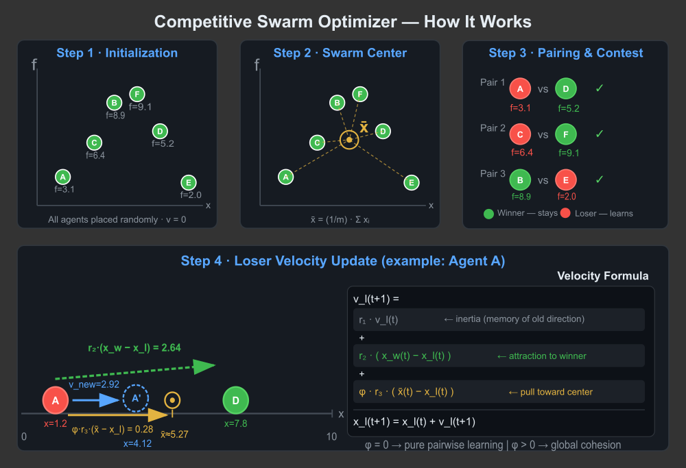
Figure 1. Illustration of how the CSO algorithm works

The illustration consists of four blocks that follow the logic of the algorithm:

• Step 1: Initialization — Six agents are randomly distributed, and their velocities are zero.
• Step 2: Swarm Center — the same agents; the dashed spokes converge toward the swarm center, x̄.
• Step 3: Pairing & Contest — three pairs; the winners are highlighted in green with a checkmark, and the losers are highlighted in red.
• Step 4: Loser Velocity Update — a specific example of agent A: the green arrow pulls toward winner D, the yellow arrow pulls toward the center, and the blue final arrow indicates the new position A′; next to it is a formula with a color-coded breakdown of the three terms.

The algorithm's complete cycle:

Initialization: distribute agents randomly, v = 0

WHILE the computation budget is not exhausted:

1. Evaluate the fitness of all agents
2. Compute the swarm center x̄
3. Randomly shuffle the agents and form pairs
4. FOR each pair (a, b):
determine the winner w and the loser l
update v_l using the velocity formula
update x_l = x_l + v_l
apply boundary control
5. Record the global best result

Return the best position found

The winners move on to the next epoch unchanged — right up until the draw in the next round pairs them with a stronger opponent. Then they themselves will become losers and will start learning too. Thus, information about good solutions gradually spreads throughout the entire population through a series of encounters — not in a directive, top-down manner, but democratically, from agent to agent.

Let's move on to writing the code for the CSO algorithm. The algorithm is implemented as the "C_AO_CSO" class, which inherits from the base class "C_AO". The architecture allows CSO to be integrated into a unified framework for testing population-based algorithms without modifying the test bench: external code interacts with the algorithm through three standard methods — Init, Moving, and Revision. The class contains one public parameter, "phi" — the attraction coefficient toward the swarm center — and a set of private arrays that support the algorithm's operation:

• V is a flattened two-dimensional array of velocities for all agents, stored in row-major order. The agent's velocity at coordinate "c" can be accessed via the helper method `Idx(i, c)`, which returns the index `i * coords + c`.
• Vmax is an array of the maximum allowable velocities for each axis. It is initialized as half the search range for the corresponding coordinate and is used to limit the velocity after each update.
• center — the swarm center vector, recalculated every epoch as the arithmetic mean of the current positions of all agents.
• rlist — an auxiliary array of indices that is shuffled by the Shuffle method before each pairing.
• nPairs — the number of pairs, equal to half the population size. If `popSize` is odd, the last agent in the current epoch does not participate in the competition.

The constructor sets the default values and registers the parameters in the "params" array, through which the test bench passes settings from outside.

The SetParams method reads values from the "params" array into the class fields. It is called by the test bench after manually changing params[i].val to synchronize the working variables with the new settings.

//————————————————————————————————————————————————————————————————————
class C_AO_CSO : public C_AO
{
public: //----------------------------------------------------------
  ~C_AO_CSO () { }
  C_AO_CSO ()
  {
    ao_name = "CSO";
    ao_desc = "Competitive Swarm Optimizer";
    ao_link = "https://www.mql5.com/en/articles/21727";

    popSize = 50;
    phi     = 0.2;

    ArrayResize (params, 2);
    params [0].name = "popSize";
    params [0].val = popSize;
    params [1].name = "phi";
    params [1].val = phi;
  }

  void SetParams ()
  {
    popSize = (int)params [0].val;
    phi     =      params [1].val;
  }

  bool Init (const double &rangeMinP  [],
             const double &rangeMaxP  [],
             const double &rangeStepP [],
             const int     epochsP = 0);

  void Moving   ();
  void Revision ();

  //------------------------------------------------------------------
  double phi; // coefficient of attraction toward the swarm center, φ ∈ [0, 1]

private: //---------------------------------------------------------
  double V       []; // particle velocities [popSize * coords]
  double Vmax    []; // velocity limit [coords]
  double center  []; // swarm center             [coords]
  int    rlist   []; // auxiliary shuffle array [popSize]
  int    nPairs;     // number of pairs = popSize / 2
  bool   initialized;

  int    Idx     (int i, int c)
  {
    return i * coords + c;
  }
  double Clamp   (double v, double lo, double hi)
  {
    return v < lo ? lo : v > hi ? hi : v;
  }
  void   Shuffle (); // Fisher-Yates shuffling of rlist
};
//————————————————————————————————————————————————————————————————————

The initialization method is called before each independent optimization run. First, it passes control to the standard initializer of the StandardInit base class, which allocates shared arrays, resets the global best result, and fills in the search ranges. After that, CSO-specific initialization is performed.

The number of pairs, nPairs, is calculated as popSize / 2. The arrays "V", "Vmax", "center", and "rlist" are allocated.

For each coordinate c, Vmax[c] = (rangeMax[c] - rangeMin[c]) * 0.5 is calculated. Limiting the velocity to half the range is standard practice in PSO-like algorithms: it prevents a situation where an agent jumps across the entire search space in a single step.

Each agent is assigned a random initial position drawn from a uniform distribution within the valid range. The initial velocities are set to zero — in exact accordance with the original article, which shows that initializing the velocities to zero yields better results than random initialization. Each agent's personal best fitness is reset to -DBL_MAX.

//————————————————————————————————————————————————————————————————————
bool C_AO_CSO::Init (const double &rangeMinP  [],
                     const double &rangeMaxP  [],
                     const double &rangeStepP [],
                     const int     epochsP = 0)
{
  if (!StandardInit (rangeMinP, rangeMaxP, rangeStepP)) return false;

  //------------------------------------------------------------------
  nPairs = popSize / 2; // A leftover agent does not participate in the competition

  ArrayResize (V,      popSize * coords);
  ArrayResize (Vmax,   coords);
  ArrayResize (center, coords);
  ArrayResize (rlist,  popSize);

  // Vmax = half the range on each axis
  for (int c = 0; c < coords; c++) Vmax [c] = (rangeMax [c] - rangeMin [c]) * 0.5;

  // Initial positions are random; velocities = 0 (as in the original article)
  for (int i = 0; i < popSize; i++)
  {
    for (int c = 0; c < coords; c++)
    {
      a [i].cP [c] = u.RNDfromCI (rangeMin [c], rangeMax [c]);
      V [Idx (i, c)] = 0.0;
    }
    a [i].fB = -DBL_MAX;
  }

  initialized = false;
  return true;
}
//————————————————————————————————————————————————————————————————————

The Moving method is responsible for preparing agent positions for external fitness evaluation. Its task is simple: to copy the current working coordinates "cP" of each agent to the coordinates "c," while applying quantization via "SeInDiSp" — a function that aligns the value to a valid grid, taking into account the "rangeStep" step size. If the step size is zero, quantization is not performed.

In CSO, the Moving method is single-phase: at each epoch, all agents simply submit their current positions "cP" for evaluation. There is no division into phases here — this makes the algorithm's structure particularly transparent.

//————————————————————————————————————————————————————————————————————
// Moving: copy the current positions from cP to c for external fitness evaluation
void C_AO_CSO::Moving ()
{
  for (int i = 0; i < popSize; i++) for (int c = 0; c < coords; c++) a [i].c [c] = u.SeInDiSp (a [i].cP [c], rangeMin [c], rangeMax [c], rangeStep [c]);
}
//————————————————————————————————————————————————————————————————————

Revision is the main method of the algorithm, executed after the outer loop has computed the fitness for all agents. It consists of four consecutive stages.

Stage 1. Updating the best results. For each agent, the system checks whether its current fitness, a[i].f, exceeds its personal best, a[i].fB. If so, the personal best is updated and the position is saved. Similarly, the global best result "fB" and the vector "cB" are updated.

Stage 2. Computing the swarm center. The "center" array is initialized to zero, and then, in a loop over all agents and coordinates, the sum of the current positions "cP" is accumulated. After dividing by "popSize," the average position of the swarm is obtained. Please note: the center is calculated based on "cP," not "c" — that is, based on the positions that will be used for movement. Not those that were passed for evaluation in "Moving." In a synchronous architecture (where Moving always copies cP → c), the difference is negligible, but it is semantically correct to compute the center based on the working coordinates.

Stage 3. Shuffling and pair formation. The "Shuffle" method is called, which randomly rearranges the indices 0..popSize-1 in the "rlist" array. After shuffling, the first half of "rlist" contains the indices of one set of participants in the pairs, and the second half contains the indices of the other set. The pair "k" is formed by the agents rlist[k] and rlist[k + nPairs].

Step 4. Pairwise competitions and updating the losers. For each pair, a winner "w" and a loser "l" are determined: since this is a maximization problem, the agent with the lower fitness value is considered the loser. Next, for each coordinate "c," three independent random numbers "r1," "r2," and "r3" are generated from [0, 1], and the velocity formula is applied:

vNew = r1 * V[idx] + r2 * (cP[w][c] - cP[l][c]) + phi * r3 * (center[c] - cP[l][c])

The resulting velocity is clamped to the range [-Vmax[c], Vmax[c]], after which a new position is calculated:

xNew = cP[l][c] + vNew

The position is also clamped to the search boundaries. The velocity and position of the winner "w" do not change.

An important implementation detail: the loser's position is updated immediately in the "cP" array, that is, in the middle of the pairwise loop. This means that if the same agent could theoretically end up as the loser in multiple pairs in a given epoch (which is impossible with proper shuffling, since each agent is included in exactly one pair), its updated position would already be visible to the other pairs. With proper shuffling, this subtlety does not cause any problems.

//————————————————————————————————————————————————————————————————————
// Revision:
//   1. Update personal/global bests
//   2. Calculate the swarm center
//   3. Generate random pairs; determine the winners and losers
//   4. Update the velocities and positions of the losers (formulas from the article)
void C_AO_CSO::Revision ()
{
  //--- 1. Updating the bests ----------------------------------------
  for (int i = 0; i < popSize; i++)
  {
    if (a [i].f > a [i].fB)
    {
      a [i].fB = a [i].f;
      ArrayCopy (a [i].cB, a [i].c, 0, 0, coords);
    }
    if (a [i].f > fB)
    {
      fB = a [i].f;
      ArrayCopy (cB, a [i].c, 0, 0, coords);
    }
  }

  initialized = true;

  //--- 2. Swarm center: center = (1/m) * Σ cP_i ---------------------
  ArrayInitialize (center, 0.0);
  for (int i = 0; i < popSize; i++) for (int c = 0; c < coords; c++) center [c] += a [i].cP [c];
  for (int c = 0; c < coords; c++) center [c] /= (double)popSize;

  //--- 3. Random pairs ------------------------------------------
  Shuffle ();

  //--- 4. Pairwise competitions and updating the losers ----------
  for (int k = 0; k < nPairs; k++)
  {
    int ai = rlist [k];
    int bi = rlist [k + nPairs];

    // Maximization: loser = the agent with lower fitness
    int li = (a [ai].f < a [bi].f) ? ai : bi; // loser
    int wi = (a [ai].f < a [bi].f) ? bi : ai; // winner

    // The velocity formula (Eq. 3 from the article):
    // v_l(t+1) = r1⊙v_l(t) + r2⊙(x_w(t) − x_l(t)) + φ·r3⊙(x̄(t) − x_l(t))
    //
    // Position formula:
    // x_l(t+1) = x_l(t) + v_l(t+1)
    for (int c = 0; c < coords; c++)
    {
      double r1 = u.RNDfromCI (0.0, 1.0);
      double r2 = u.RNDfromCI (0.0, 1.0);
      double r3 = u.RNDfromCI (0.0, 1.0);

      int idx = Idx (li, c);

      double vNew =          r1 * V [idx]
                             +        r2 * (a [wi].cP [c] - a [li].cP [c])
                             + phi  * r3 * (center [c] - a [li].cP [c]);

      vNew = Clamp (vNew, -Vmax [c], Vmax [c]);

      double xNew = Clamp (a [li].cP [c] + vNew, rangeMin [c], rangeMax [c]);

      V [idx] = vNew;
      a [li].cP [c] = xNew;
      // The winner's position, cP[wi], remains unchanged
    }
  }
}
//————————————————————————————————————————————————————————————————————

The Shuffle method implements the Fisher–Yates algorithm for uniformly shuffling an array of integers. First, "rlist" is filled with the sequence 0, 1, 2, ..., popSize-1. Then, in a loop running from the end to the beginning, each element is swapped with a random element from the prefix that has not yet been processed. The result is a uniform random permutation that ensures that pairing in each epoch is completely unpredictable.

The random number generator is called via u.RNDfromCI (0.0, 1.0), where "u" is an instance of the C_AO_Utilities helper class from the base class. The index "j" is capped at "i" to prevent going out of array bounds when rounding a real number to an integer.

Helper methods:

Idx (i, c) — returns the linear index in the one-dimensional array "V" for agent "i" and coordinate "c".

Clamp (v, lo, hi) — clamps the value "v" to the range [lo, hi]. It is applied to both velocities and positions after updating.

//————————————————————————————————————————————————————————————————————
// Fisher-Yates shuffling of the `rlist` array
void C_AO_CSO::Shuffle ()
{
  for (int i = 0; i < popSize; i++) rlist [i] = i;
  for (int i = popSize - 1; i > 0; i--)
  {
    int j = (int)(u.RNDfromCI (0.0, 1.0) * (i + 1));
    if (j > i) j = i;
    int tmp    = rlist [i];
    rlist [i] = rlist [j];
    rlist [j] = tmp;
  }
}
//————————————————————————————————————————————————————————————————————

Test Results

CSO|Competitive Swarm Optimizer|50.0|0.2|
=============================
5 Hilly's; Func runs: 10000; result: 0.9029155571810208
25 Hilly's; Func runs: 10000; result: 0.6188702055480547
500 Hilly's; Func runs: 10000; result: 0.29830471226794253
=============================
5 Forest's; Func runs: 10000; result: 0.9998176263259818
25 Forest's; Func runs: 10000; result: 0.6458134365888859
500 Forest's; Func runs: 10000; result: 0.2397479908923888
=============================
5 Megacity's; Func runs: 10000; result: 0.633846153846154
25 Megacity's; Func runs: 10000; result: 0.4055384615384615
500 Megacity's; Func runs: 10000; result: 0.12852307692307804
=============================
Overall score: 4.87338 (54.15%)

Visualization of the CSO algorithm in action. Our visualization has changed due to its implementation in 3D. Now we can see not only the functions with 3D color coding, but also the the trajectory of the best solution throughout each optimization run. Below, we will examine the implementation code for the 3D test bench.

CSO on the Hilly test function

CSO on the Forest test function

CSO on the Megacity test function

CSO on the Rastrigin test function

CSO on the Ackley test function

The C_TestStand3D class is a 3D test bench for metaheuristics. Along with the classic two-dimensional test bench (C_TestStand), which displays the function landscape as a heat map and a convergence graph, the C_TestStand3D 3D visualizer has been added to the toolkit for this series. It overlays the left square panel of the two-dimensional test bench with an interactive DirectX surface and operates in parallel with it: the right panel with the convergence graph remains visible through the two-dimensional canvas unchanged.

The function surface is built using the BuildSurface() method, which takes a “C_Function” object and a mesh resolution parameter (by default, 80 vertices per axis; allowable range: 10–200). The color scheme is CS_COLD_TO_HOT: blue corresponds to the minimum value of the function, red to the maximum, and it is visually consistent with the heat map of the two-dimensional test bench. Population agents are passed via the SetAgents() method as an array of (x, y) pairs and are projected onto the surface manually using a view × projection matrix, since CCanvas3D's two-dimensional primitives are not part of the DirectX pipeline. The best agent is marked with a white circle of increased radius.

The fundamental difference between a three-dimensional test bench and a two-dimensional one is the presence of a best-solution trail — a tool that is not available in a flat representation. The trail records the world coordinates of the best agent at each epoch in a circular buffer with a capacity of 600 points and displays the accumulated history as a continuous gold line (#FFC828). The opacity of the line increases from the beginning of the trail to its end: older positions are rendered almost transparent (alpha ≈ 0x30), while newer ones are rendered more opaque (alpha ≈ 0xE0), allowing you to assess at a glance the direction and velocity of the best solution’s movement across the landscape. To create the illusion of thickness, each segment is duplicated with a vertical offset of one pixel. The trail is automatically reset when the test function is changed (BuildSurface) and at the start of each independent repeated run (ResetTrail), so the screen always displays only the history of the current independent test.

For now, camera control is planned via left-button dragging (azimuth and tilt rotation), the mouse wheel, and double-clicking (reset to the default position); however, the image is currently static, and the current implementation also reserves space in the code for future changes. The LookAt and perspective projection matrices are implemented using the portable matrix helpers _LookAtLH and _PerspLH, without relying on external DX utilities, since MQL5 requires DXVector3 structures to be passed only by reference and does not support matrix fields in _11/_12 notation. The agents’ colors are generated by the _HSL function, which uniformly distributes the spectrum hues from blue (the first agent) to red (the last) with saturation S = 1 and lightness L = 0.5.

//+------------------------------------------------------------------+
//|                                                  TestStand3D.mqh |
//|  3D visualization panel for the metaheuristics test bench        |
//|                                                                  |
//|  Order of #include statements in the script:                     |
//|    1. TestStandFunctions.mqh  — C_TestStand (2D test stand)      |
//|    2. TestFunctions.mqh       — C_Function, GenerateDataFixedSize|
//|    3. TestStand3D.mqh         — this file                        |
//|    4. Optimization algorithm                                     |
//+------------------------------------------------------------------+

#include <Canvas\Canvas3D.mqh>
#include <Canvas\DX\DXSurface.mqh>
#include <Math\AOs\TestFunctions.mqh>

//--- Camera parameters (can be changed)
#define S3D_DIST_DEF      35.0    // default distance
#define S3D_DIST_MIN      12.0    // minimum zoom-in
#define S3D_DIST_MAX      80.0    // maximum zoom-out
#define S3D_PITCH_DEF     0.45f   // default camera pitch (~26°)
#define S3D_FOV           0.5236f // field of view = π/6 (30°)
//--- Surface half-extents in world coordinates
#define S3D_SX            10.0f
#define S3D_SY             5.0f
#define S3D_SZ            10.0f

//--- 3D panel background color
#define S3D_BG            0xFF0D0D1A

//+------------------------------------------------------------------+
//| S3DTrailPt — best-solution trail point (world coordinates)       |
//+------------------------------------------------------------------+
struct S3DTrailPt
{
  float wx, wy, wz;
};

//+------------------------------------------------------------------+
//| S3DAgent — population agent (world coordinates + color)          |
//+------------------------------------------------------------------+
struct S3DAgent
{
  float             wx, wy, wz;
  uint              clr;        // ARGB
  bool              is_best;    // best agent — special rendering
};

//+------------------------------------------------------------------------+
//| C_TestStand3D                                                          |
//|                                                                        |
//| Displays the left (H×H) panel of the test bench as an interactive      |
//| 3D function surface with agent projections and the best-solution trail.|
//|                                                                        |
//| Controls (EA context, events via OnChartEvent):                        |
//|   LMB-drag      — rotate the camera                                    |
//|   Scroll        — zoom                                                 |
//|   Double-click  — reset the camera to its default position             |
//+------------------------------------------------------------------------+
class C_TestStand3D
{
  //--- DX objects
  CCanvas3D  m_cv;
  CDXSurface m_surf;

  //--- canvas parameters
  string m_name;
  int    m_x, m_y, m_w, m_h;
  bool   m_surf_ok;
  bool   m_vis;
  bool   m_shutdown_done;
  int    m_grid;

  //--- camera parameters
  float  m_pitch;      // tilt (around the X-axis)
  float  m_yaw;        // azimuth (around Y)
  double m_dist;       // distance from the center of the scene
  int    m_mx, m_my;   // previous mouse position (local)

  //--- view×projection matrix for manually projecting agents onto the screen
  DXMatrix m_vp;

  //--- function domain range (for mapping agents to world coordinates)
  double m_fxMin, m_fxMax, m_fyMin, m_fyMax;

  //--- agents of the current epoch
  S3DAgent m_ag [];
  int      m_nAg;

  //--- best-solution trail (ring buffer)
  S3DTrailPt m_trail [];
  int        m_trailLen;
  int        m_trailMax;

public:
  C_TestStand3D  ();
  ~C_TestStand3D ()
  {
    Shutdown ();
  }

  //--- life cycle
  bool              Init (const string name, int x, int y, int w, int h);
  void              Shutdown ();

  //--- content
  // grid — number of vertices along one axis (10..200); call when the function changes
  bool              BuildSurface (C_Function &func, int grid = 80);
  // args[] = [x0, y0, x1, y1, …] (number of pairs); best_idx = -1 → no highlighting
  void              SetAgents (double &args [], int count,
                               C_Function &func, int best_idx = -1);
  // a single render frame
  void              Redraw ();
  // reset the best-solution trail (call at the beginning of each new test)
  void              ResetTrail ()
  {
    m_trailLen = 0;
  }

  //--- events (route from OnChartEvent to the EA)
  void              OnMouseMove (int chart_x, int chart_y, uint flags);
  void              OnMouseWheel (double delta);
  void              OnDblClick ();
  // dt in seconds; pass a fixed virtual step in the script
  void              OnTimer (double dt);

  //--- visibility and size
  void              Show (bool v);
  bool              IsVisible () const
  {
    return m_vis;
  }
  string            GetName ()   const
  {
    return m_name;
  }
  void              Resize (int new_w, int new_h);

private:
  //--- recalculation of the camera and VP matrices
  void              _CamUpdate ();
  //--- projection of a world point → screen pixels; false = off-screen
  bool              _Project (float wx, float wy, float wz, int &sx, int &sy);
  //--- rendering the best-solution trail and agents
  void              _DrawTrail ();
  void              _DrawAgents ();

  //--- matrix helpers (portable, without external DX functions)
  // Note: DXMatrix in MQL5 stores elements as m[row][col]
  //           DXVector3 is passed by reference only
  static void       _LookAtLH (DXMatrix &M, DXVector3 &eye, DXVector3 &tgt, DXVector3 &up);
  static void       _PerspLH (DXMatrix &M, float fov, float aspect, float zn, float zf);
  static void       _MulMat (DXMatrix &C, DXMatrix &A, DXMatrix &B);

  //--- rainbow color by agent index: h_deg ∈ [0,360] → ARGB (S=1, L=0.5)
  static uint       _HSL (int h_deg);
};

//+------------------------------------------------------------------+
C_TestStand3D::C_TestStand3D ()
  : m_surf_ok (false), m_vis (false), m_shutdown_done (false),
    m_nAg (0), m_grid (80),
    m_pitch (S3D_PITCH_DEF), m_yaw (0.0f), m_dist (S3D_DIST_DEF),
    m_mx (-1), m_my (-1),
    m_fxMin (0), m_fxMax (1), m_fyMin (0), m_fyMax (1),
    m_trailLen (0), m_trailMax (600)
{
  ArrayResize (m_trail, m_trailMax);
}

//+------------------------------------------------------------------+
bool C_TestStand3D::Init (const string name, int x, int y, int w, int h)
{
  m_name = name;
  m_x = x;
  m_y = y;
  m_w = w;
  m_h = h;

  ResetLastError ();
  if (!m_cv.CreateBitmapLabel (m_name, m_x, m_y, m_w, m_h,
                               COLOR_FORMAT_ARGB_NORMALIZE))
  {
    PrintFormat ("C_TestStand3D::Init – error CreateBitmapLabel: %d",
                 GetLastError ());
    return false;
  }

  m_cv.ProjectionMatrixSet (S3D_FOV, (float)m_w / m_h, 0.1f, 200.0f);

  DXVector3 tgt = DXVector3 (0.0f, 0.0f, 0.0f);
  DXVector3 up  = DXVector3 (0.0f, 1.0f, 0.0f);
  m_cv.ViewTargetSet (tgt);
  m_cv.ViewUpDirectionSet (up);

  m_cv.LightColorSet (DXColor (1.0f, 0.97f, 0.88f, 0.32f));
  m_cv.AmbientColorSet (DXColor (0.82f, 0.88f, 1.0f, 0.72f));

  _CamUpdate ();

  ObjectSetInteger (0, m_name, OBJPROP_HIDDEN,     true);
  ObjectSetInteger (0, m_name, OBJPROP_SELECTABLE, false);
  return true;
}

//+------------------------------------------------------------------+
void C_TestStand3D::Shutdown ()
{
  if (m_shutdown_done) return;
  m_shutdown_done = true;
  m_surf.Shutdown ();
  // We do not call m_cv.Destroy() — the CCanvas3D destructor will do it itself.
  // Calling Destroy() twice resulted in Abnormal termination.
  ObjectDelete (0, m_name);
}

//+------------------------------------------------------------------+
bool C_TestStand3D::BuildSurface (C_Function &func, int grid)
{
  m_grid = (int)MathMax (10.0, MathMin (200.0, (double)grid));

  m_fxMin = func.GetMinRangeX ();
  m_fxMax = func.GetMaxRangeX ();
  m_fyMin = func.GetMinRangeY ();
  m_fyMax = func.GetMaxRangeY ();

  double buf [];
  if (!GenerateDataFixedSize (m_grid, m_grid, func, buf))
  {
    Print ("C_TestStand3D::BuildSurface – GenerateDataFixedSize failed");
    return false;
  }

  const float VAL_RANGE = 1.0f;   // The C_Function normalizes values to the range [0,1]
  DXVector3 bMin = DXVector3 (-S3D_SX, -S3D_SY, -S3D_SZ);
  DXVector3 bMax = DXVector3 (S3D_SX,  S3D_SY,  S3D_SZ);
  DXVector2 uv   = DXVector2 (1.0f, 1.0f);

  if (!m_surf_ok)
  {
    if (!m_surf.Create (m_cv.DXDispatcher (), m_cv.InputScene (),
                        buf, (uint)m_grid, (uint)m_grid,
                        VAL_RANGE, bMin, bMax, uv,
                        CDXSurface::SF_TWO_SIDED | CDXSurface::SF_USE_NORMALS))
    {
      Print ("C_TestStand3D::BuildSurface – CDXSurface::Create failed");
      return false;
    }
    // CDXSurface::Create does not accept a color scheme → Update immediately,
    // Otherwise, the first function is displayed without a gradient (gray).
    m_surf.Update (buf, (uint)m_grid, (uint)m_grid,
                   VAL_RANGE, bMin, bMax, uv,
                   CDXSurface::SF_TWO_SIDED | CDXSurface::SF_USE_NORMALS,
                   CDXSurface::CS_COLD_TO_HOT);
    m_surf.SpecularColorSet (DXColor (1.0f, 1.0f, 1.0f, 0.55f));
    m_cv.ObjectAdd (&m_surf);
    m_surf_ok = true;
  }
  else
  {
    m_surf.Update (buf, (uint)m_grid, (uint)m_grid,
                   VAL_RANGE, bMin, bMax, uv,
                   CDXSurface::SF_TWO_SIDED | CDXSurface::SF_USE_NORMALS,
                   CDXSurface::CS_COLD_TO_HOT);
  }

  m_nAg      = 0;
  m_trailLen = 0;   // The trail is reset when the function changes
  return true;
}

//+------------------------------------------------------------------+
void C_TestStand3D::SetAgents (double &args [], int count,
                               C_Function &func, int best_idx)
{
  m_nAg = MathMax (0, count);
  if (m_nAg == 0) return;

  ArrayResize (m_ag, m_nAg);

  double rx = m_fxMax - m_fxMin;
  if (rx < 1e-9) rx = 1e-9;
  double ry = m_fyMax - m_fyMin;
  if (ry < 1e-9) ry = 1e-9;

  for (int i = 0; i < m_nAg; i++)
  {
    // clamping to the valid range
    double ax = MathMax (m_fxMin, MathMin (m_fxMax, args [i * 2]));
    double ay = MathMax (m_fyMin, MathMin (m_fyMax, args [i * 2 + 1]));

    // mapping: function domain → world coordinates of the surface
    float wx = (float)(-S3D_SX + (ax - m_fxMin) / rx * 2.0 * S3D_SX);
    float wz = (float)(-S3D_SZ + (ay - m_fyMin) / ry * 2.0 * S3D_SZ);

    // height: normalized function value [0,1] → world Y + offset
    double fv = MathMax (0.0, MathMin (1.0, func.Core (ax, ay)));
    float  wy = (float)(-S3D_SY + fv * 2.0 * S3D_SY) + 0.22f;

    m_ag [i].wx      = wx;
    m_ag [i].wy      = wy;
    m_ag [i].wz      = wz;
    m_ag [i].is_best = (i == best_idx);
    // rainbow color: blue (i=0) → red (i=last)
    m_ag [i].clr     = _HSL ((int)(270.0 * i / MathMax (1, m_nAg - 1)));

    // add the best position to the trail
    if (i == best_idx && best_idx >= 0)
    {
      if (m_trailLen < m_trailMax)
      {
        m_trail [m_trailLen].wx = wx;
        m_trail [m_trailLen].wy = wy;
        m_trail [m_trailLen].wz = wz;
        m_trailLen++;
      }
      else
      {
        // buffer is full — shift by 1; the oldest point is discarded
        for (int t = 0; t < m_trailMax - 1; t++) m_trail [t] = m_trail [t + 1];
        m_trail [m_trailMax - 1].wx = wx;
        m_trail [m_trailMax - 1].wy = wy;
        m_trail [m_trailMax - 1].wz = wz;
      }
    }
  }
}

//+------------------------------------------------------------------+
void C_TestStand3D::Redraw ()
{
  if (!m_vis || !m_surf_ok) return;
  m_cv.Render (DX_CLEAR_COLOR | DX_CLEAR_DEPTH, S3D_BG);
  _DrawTrail ();    // trail under the agents
  _DrawAgents ();
  m_cv.Update ();
}

//+------------------------------------------------------------------+
void C_TestStand3D::_CamUpdate ()
{
  // Rotate the base position (0, 0, -dist) around the X-axis (pitch), then around the Y-axis (yaw)
  DXVector4 cam = DXVector4 (0.0f, 0.0f, -(float)m_dist, 1.0f);
  DXVector4 lgt = DXVector4 (0.25f, -0.45f, 1.0f, 0.0f);
  DXMatrix  rot;

  DXMatrixRotationX (rot, m_pitch);
  DXVec4Transform   (cam, cam, rot);
  DXVec4Transform   (lgt, lgt, rot);

  DXMatrixRotationY (rot, m_yaw);
  DXVec4Transform (cam, cam, rot);
  DXVec4Transform (lgt, lgt, rot);

  DXVector3 eye = DXVector3 (cam);
  DXVector3 ld  = DXVector3 (lgt);
  DXVector3 tgt = DXVector3 (0.0f, 0.0f, 0.0f);
  DXVector3 up  = DXVector3 (0.0f, 1.0f, 0.0f);

  // Update all camera parameters so that CCanvas3D recalculates the view matrix
  m_cv.ViewPositionSet (eye);
  m_cv.ViewTargetSet (tgt);
  m_cv.ViewUpDirectionSet (up);
  m_cv.LightDirectionSet (ld);

  // Build a VP matrix for manually projecting agents in _Project()
  DXMatrix view, proj;
  _LookAtLH (view, eye, tgt, up);
  _PerspLH (proj, S3D_FOV, (float)m_w / m_h, 0.1f, 200.0f);
  _MulMat (m_vp, view, proj);
}

//+------------------------------------------------------------------+
bool C_TestStand3D::_Project (float wx, float wy, float wz,
                              int &sx, int &sy)
{
  DXVector4 p = DXVector4 (wx, wy, wz, 1.0f);
  DXVec4Transform (p, p, m_vp);
  if (p.w < 0.01f) return false;

  float nx = p.x / p.w;
  float ny = p.y / p.w;
  if (nx < -1.1f || nx > 1.1f || ny < -1.1f || ny > 1.1f) return false;

  sx = (int)((nx + 1.0f) * 0.5f * m_w);
  sy = (int)((1.0f - ny) * 0.5f * m_h);
  return true;
}

//+------------------------------------------------------------------------------------+
//| _DrawTrail                                                                         |
//| Gold line (#FFC828) showing the history of positions of the best agent.            |
//| Transparency gradient: old points have alpha ≈ 0x30, new ones have alpha ≈ 0xE0.   |
//| Double line (offset +1px along Y) — visual thickness.                              |
//+------------------------------------------------------------------------------------+
void C_TestStand3D::_DrawTrail ()
{
  if (m_trailLen < 2) return;

  int  px = 0, py = 0, cx = 0, cy = 0;
  bool hasPrev = false;

  for (int t = 0; t < m_trailLen; t++)
  {
    if (!_Project (m_trail [t].wx, m_trail [t].wy, m_trail [t].wz, cx, cy))
    {
      hasPrev = false;   // break when a point goes outside the viewport
      continue;
    }

    if (!hasPrev)
    {
      px = cx;
      py = cy;
      hasPrev = true;
      continue;
    }

    double ratio = (double)t / (double)(m_trailLen - 1);
    uint   alpha = (uint)(0x30 + ratio * 0xB0);   // 0x30 → 0xE0

    uint clr  = (alpha        << 24) | 0x00FFC828;
    uint clrT = ((alpha >> 1) << 24) | 0x00FFC828;  // shadow +1px

    m_cv.LineAA (px, py,     cx, cy,     clr);
    m_cv.LineAA (px, py + 1, cx, cy + 1, clrT);

    px = cx;
    py = cy;
  }
}

//+------------------------------------------------------------------+
//| _DrawAgents                                                      |
//| Standard agent: colored circle with r=4 and a black outline.     |
//| Best agent: white circle with r=7 + heavy shadow.                |
//+------------------------------------------------------------------+
void C_TestStand3D::_DrawAgents ()
{
  for (int i = 0; i < m_nAg; i++)
  {
    int sx, sy;
    if (!_Project (m_ag [i].wx, m_ag [i].wy, m_ag [i].wz, sx, sy)) continue;

    if (m_ag [i].is_best)
    {
      m_cv.FillCircle (sx, sy, 7, 0xFFFFFFFF);
      m_cv.Circle     (sx, sy, 7, 0xFF000000);
      m_cv.Circle     (sx, sy, 8, 0xFF000000);
      m_cv.Circle     (sx, sy, 9, 0x88000000);
    }
    else
    {
      m_cv.FillCircle (sx, sy, 4, m_ag [i].clr);
      m_cv.Circle     (sx, sy, 4, 0xFF000000);
      m_cv.Circle     (sx, sy, 5, 0x55000000);
    }
  }
}

//+------------------------------------------------------------------+
void C_TestStand3D::OnMouseMove (int chart_x, int chart_y, uint flags)
{
  int lx = chart_x - m_x;
  int ly = chart_y - m_y;

  if ((flags & 1) == 1)   // LMB pressed
  {
    if (m_mx >= 0)
    {
      m_yaw   += (lx - m_mx) / 240.0f;
      m_pitch += (ly - m_my) / 240.0f;
      // Tilt limit: ±86°
      float pMax = (float)(DX_PI * 0.48);
      if (m_pitch < -pMax) m_pitch = -pMax;
      if (m_pitch >  pMax) m_pitch =  pMax;
      _CamUpdate ();
    }
    m_mx = lx;
    m_my = ly;
  }
  else
  {
    m_mx = -1;
    m_my = -1;
  }
}

//+------------------------------------------------------------------+
void C_TestStand3D::OnMouseWheel (double delta)
{
  m_dist *= (1.0 - delta * 0.0012);
  m_dist  = MathMax (S3D_DIST_MIN, MathMin (S3D_DIST_MAX, m_dist));
  _CamUpdate ();
}

//+------------------------------------------------------------------+
void C_TestStand3D::OnDblClick ()
{
  m_pitch = S3D_PITCH_DEF;
  m_yaw   = 0.0f;
  m_dist  = S3D_DIST_DEF;
  _CamUpdate ();
}

//+------------------------------------------------------------------+
void C_TestStand3D::OnTimer (double dt)
{
  // Reserved for future implementation of auto-rotation
}

//+------------------------------------------------------------------+
void C_TestStand3D::Show (bool v)
{
  m_vis = v;
  ObjectSetInteger (0, m_name, OBJPROP_HIDDEN, !v);
  ChartRedraw ();
}

//+------------------------------------------------------------------+
void C_TestStand3D::Resize (int new_w, int new_h)
{
  if (new_w == m_w && new_h == m_h) return;
  m_w = new_w;
  m_h = new_h;
  m_cv.Resize (m_w, m_h);
  DXContextSetSize (m_cv.DXContext (), m_w, m_h);
  m_cv.ProjectionMatrixSet (S3D_FOV, (float)m_w / m_h, 0.1f, 200.0f);
  _CamUpdate ();
}

//══════════════════════════════════════════════════════════════════
//  Matrix helpers
//
//  DXMatrix in MQL5 stores elements as m[row][col], NOT as _11/_12
//  DXVector3 is passed by reference only (objects are passed by reference only in MQL5)
//  All matrices are row-major, left-handed (DirectX convention)
//══════════════════════════════════════════════════════════════════

//--- LookAt LH: equivalent to D3DXMatrixLookAtLH
void C_TestStand3D::_LookAtLH (DXMatrix &M, DXVector3 &eye, DXVector3 &tgt, DXVector3 &up)
{
  // z = normalize(tgt - eye) — the "forward" axis
  float zx = tgt.x - eye.x, zy = tgt.y - eye.y, zz = tgt.z - eye.z;
  float zl = (float)MathSqrt (zx * zx + zy * zy + zz * zz);
  if (zl < 1e-7f) zl = 1e-7f;
  zx /= zl;
  zy /= zl;
  zz /= zl;

  // x = normalize(cross(up, z))  — the "right" axis
  float xx = up.y * zz - up.z * zy;
  float xy = up.z * zx - up.x * zz;
  float xz = up.x * zy - up.y * zx;
  float xl = (float)MathSqrt (xx * xx + xy * xy + xz * xz);
  if (xl < 1e-7f) xl = 1e-7f;
  xx /= xl;
  xy /= xl;
  xz /= xl;

  // y = cross(z, x) — the orthogonalized "up" axis
  float yx = zy * xz - zz * xy;
  float yy = zz * xx - zx * xz;
  float yz = zx * xy - zy * xx;

  // translation component (dot products of the camera's position with the axes)
  float dx = -(xx * eye.x + xy * eye.y + xz * eye.z);
  float dy = -(yx * eye.x + yy * eye.y + yz * eye.z);
  float dz = -(zx * eye.x + zy * eye.y + zz * eye.z);

  M.m [0] [0] = xx;
  M.m [0] [1] = yx;
  M.m [0] [2] = zx;
  M.m [0] [3] = 0.0f;
  M.m [1] [0] = xy;
  M.m [1] [1] = yy;
  M.m [1] [2] = zy;
  M.m [1] [3] = 0.0f;
  M.m [2] [0] = xz;
  M.m [2] [1] = yz;
  M.m [2] [2] = zz;
  M.m [2] [3] = 0.0f;
  M.m [3] [0] = dx;
  M.m [3] [1] = dy;
  M.m [3] [2] = dz;
  M.m [3] [3] = 1.0f;
}

//--- Perspective LH: equivalent to D3DXMatrixPerspectiveFovLH
void C_TestStand3D::_PerspLH (DXMatrix &M,
                              float fov, float aspect, float zn, float zf)
{
  float ys = 1.0f / (float)MathTan (fov * 0.5);
  float xs = ys / aspect;
  float zr = zf / (zf - zn);

  M.m [0] [0] = xs;
  M.m [0] [1] = 0.0f;
  M.m [0] [2] = 0.0f;
  M.m [0] [3] = 0.0f;
  M.m [1] [0] = 0.0f;
  M.m [1] [1] = ys;
  M.m [1] [2] = 0.0f;
  M.m [1] [3] = 0.0f;
  M.m [2] [0] = 0.0f;
  M.m [2] [1] = 0.0f;
  M.m [2] [2] = zr;
  M.m [2] [3] = 1.0f;
  M.m [3] [0] = 0.0f;
  M.m [3] [1] = 0.0f;
  M.m [3] [2] = -zn * zr;
  M.m [3] [3] = 0.0f;
}

//--- C = A × B (row-major)
void C_TestStand3D::_MulMat (DXMatrix &C, DXMatrix &A, DXMatrix &B)
{
  C.m [0] [0] = A.m [0] [0] * B.m [0] [0] + A.m [0] [1] * B.m [1] [0] + A.m [0] [2] * B.m [2] [0] + A.m [0] [3] * B.m [3] [0];
  C.m [0] [1] = A.m [0] [0] * B.m [0] [1] + A.m [0] [1] * B.m [1] [1] + A.m [0] [2] * B.m [2] [1] + A.m [0] [3] * B.m [3] [1];
  C.m [0] [2] = A.m [0] [0] * B.m [0] [2] + A.m [0] [1] * B.m [1] [2] + A.m [0] [2] * B.m [2] [2] + A.m [0] [3] * B.m [3] [2];
  C.m [0] [3] = A.m [0] [0] * B.m [0] [3] + A.m [0] [1] * B.m [1] [3] + A.m [0] [2] * B.m [2] [3] + A.m [0] [3] * B.m [3] [3];
  C.m [1] [0] = A.m [1] [0] * B.m [0] [0] + A.m [1] [1] * B.m [1] [0] + A.m [1] [2] * B.m [2] [0] + A.m [1] [3] * B.m [3] [0];
  C.m [1] [1] = A.m [1] [0] * B.m [0] [1] + A.m [1] [1] * B.m [1] [1] + A.m [1] [2] * B.m [2] [1] + A.m [1] [3] * B.m [3] [1];
  C.m [1] [2] = A.m [1] [0] * B.m [0] [2] + A.m [1] [1] * B.m [1] [2] + A.m [1] [2] * B.m [2] [2] + A.m [1] [3] * B.m [3] [2];
  C.m [1] [3] = A.m [1] [0] * B.m [0] [3] + A.m [1] [1] * B.m [1] [3] + A.m [1] [2] * B.m [2] [3] + A.m [1] [3] * B.m [3] [3];
  C.m [2] [0] = A.m [2] [0] * B.m [0] [0] + A.m [2] [1] * B.m [1] [0] + A.m [2] [2] * B.m [2] [0] + A.m [2] [3] * B.m [3] [0];
  C.m [2] [1] = A.m [2] [0] * B.m [0] [1] + A.m [2] [1] * B.m [1] [1] + A.m [2] [2] * B.m [2] [1] + A.m [2] [3] * B.m [3] [1];
  C.m [2] [2] = A.m [2] [0] * B.m [0] [2] + A.m [2] [1] * B.m [1] [2] + A.m [2] [2] * B.m [2] [2] + A.m [2] [3] * B.m [3] [2];
  C.m [2] [3] = A.m [2] [0] * B.m [0] [3] + A.m [2] [1] * B.m [1] [3] + A.m [2] [2] * B.m [2] [3] + A.m [2] [3] * B.m [3] [3];
  C.m [3] [0] = A.m [3] [0] * B.m [0] [0] + A.m [3] [1] * B.m [1] [0] + A.m [3] [2] * B.m [2] [0] + A.m [3] [3] * B.m [3] [0];
  C.m [3] [1] = A.m [3] [0] * B.m [0] [1] + A.m [3] [1] * B.m [1] [1] + A.m [3] [2] * B.m [2] [1] + A.m [3] [3] * B.m [3] [1];
  C.m [3] [2] = A.m [3] [0] * B.m [0] [2] + A.m [3] [1] * B.m [1] [2] + A.m [3] [2] * B.m [2] [2] + A.m [3] [3] * B.m [3] [2];
  C.m [3] [3] = A.m [3] [0] * B.m [0] [3] + A.m [3] [1] * B.m [1] [3] + A.m [3] [2] * B.m [2] [3] + A.m [3] [3] * B.m [3] [3];
}

//--- HSL→ARGB with S=1, L=0.5 (pure spectrum)
uint C_TestStand3D::_HSL (int h_deg)
{
  double hue = h_deg / 360.0;
  uint   ch [3];
  double off [3];
  off [0] = 1.0 / 3.0;
  off [1] = 0.0;
  off [2] = -1.0 / 3.0;

  for (int i = 0; i < 3; i++)
  {
    double vh = hue + off [i];
    if (vh < 0.0) vh += 1.0;
    if (vh > 1.0) vh -= 1.0;

    double v;
    if     (6.0 * vh < 1.0) v = 6.0 * vh;
    else if (2.0 * vh < 1.0) v = 1.0;
    else if (3.0 * vh < 2.0) v = (2.0 / 3.0 - vh) * 6.0;
    else                     v = 0.0;

    ch [i] = (uint)(v * 255.0);
  }

  return 0xFF000000 | (ch [0] << 16) | (ch [1] << 8) | ch [2];
}
//+------------------------------------------------------------------+
//+------------------------------------------------------------------+

The test script underwent only the minimum necessary changes, maintaining full backward compatibility with the 2D test bench and leaving the logic of the optimization algorithm unchanged.

The order of the #include directives is now strictly fixed. The TestStand3D.mqh header file is included third — after TestStandFunctions.mqh and TestFunctions.mqh — because it uses the C_Function"type and the GenerateDataFixedSize function declared in the preceding header files. The optimization algorithm is included last, after all the test benches.

Two new input parameters have been added: Use3D_P (a Boolean flag that enables or disables 3D visualization) and Grid3D_P (surface grid resolution; valid range: 20–150). Both parameters have been moved to a separate group called TestStand_5, along with the existing DelayInMS_P and Video_P, which preserves the familiar layout of the input parameters dialog.

In OnStart, after the 2D test bench is initialized, a C_TestStand3D object is created via a pointer. The pointer is intentionally declared as "NULL" and is assigned only when Use3D_P = true; therefore, when 3D rendering is disabled, the overhead is zero. If the 3D test bench's Init() function returns an error — for example, due to a lack of DirectX hardware support — the pointer is immediately released and set to NULL, and the script continues to run in standard 2D mode. Every time the test function changes, BuildSurface() is called, rebuilding the surface and resetting the trail; after that, the test bench is made visible using Show(true).

The "FuncTests" function now has an additional parameter — a C_TestStand3D *st3 pointer, which may be "NULL." All code related to it is protected by the if (st3 != NULL) check, so the function signature remains compatible with any script that does not use the 3D test bench. The ag3D[] agent coordinate buffer is allocated once after ao.Init(), not at every epoch. At the same point, immediately after agCnt is calculated, st3. ResetTrail() is called to reset the trail at the start of each independent retest. The on-screen best-solution trail always displays the history of only the current run, not a combined history of all previous runs.

Within the epoch loop, after the 2D rendering is complete, a 3D visualization block has been added. It fills the ag3D buffer with the c[0] and c[1] coordinates of each agent, finds the index of the agent with the best fitness value using a linear search, passes all of this to SetAgents(), and then calls Redraw(). The 2D rendering remains unaffected and is performed in the same way as in the original script.

Finalization is organized in accordance with the specific characteristics of the "CCanvas3D" lifecycle. The 3D test bench is hidden using Show(false) and destroyed using delete; an explicit call to Shutdown() is intentionally omitted: the class destructor calls it automatically via a guard flag, and a double call to Destroy() would cause the script to terminate abnormally with an "Abnormal termination" message. The 2D test bench, by contrast, requires an explicit call to `ST.Canvas.Destroy()` before termination — without it, the bitmap object remains on the chart after the script finishes running.

//────────────────────────────────────────────────────────────────────
void OnStart ()
{
  //--- Create and configure the algorithm
  C_AO *AO = new C_AO_CSO ();
  AO.params [0].val = PopSize_P;
  AO.params [1].val = Phi_P;
  AO.SetParams ();
  Print (AO.GetName (), "|", AO.GetDesc (), "|", AO.GetParams ());

  //--- 2D test bench (width 750, height 375 — standard)
  C_TestStand ST;
  ST.Init (750, 375);

  //--- 3D test bench
  //    Covers the left H×H panel of the 2D test bench (function heat map).
  //    The right panel with convergence remains visible through the 2D canvas.
  //    ST.H = test bench height (= WscrFunc/HscrFunc = H-2 = 373).
  C_TestStand3D *ST3 = NULL;
  if (Use3D_P)
  {
    ST3 = new C_TestStand3D ();
    int side = ST.H;  // square left panel
    if (!ST3.Init ("__3DView__", 5, 30, side, side))
    {
      Print ("C_TestStand3D: Init failed — 3D mode disabled");
      delete ST3;
      ST3 = NULL;
    }
  }

  //==================================================================
  double allScore = 0.0;
  double allTests = 0.0;

  if (Function1 != NONE_Func)
  {
    C_Function *F = SelectFunction (Function1);
    if (F != NULL)
    {
      Print ("=============================");
      ST.CanvasErase ();
      // When the function changes, recalculate the 3D surface
      if (ST3 != NULL)
      {
        ST3.BuildSurface (*F, Grid3D_P);
        ST3.Show (true);
      }
      FuncTests (AO, ST, ST3, *F, Test1FuncRuns_P, clrLime,      allScore, allTests);
      FuncTests (AO, ST, ST3, *F, Test2FuncRuns_P, clrAqua,      allScore, allTests);
      FuncTests (AO, ST, ST3, *F, Test3FuncRuns_P, clrOrangeRed, allScore, allTests);
      delete F;
    }
  }

  if (Function2 != NONE_Func)
  {
    C_Function *F = SelectFunction (Function2);
    if (F != NULL)
    {
      Print ("=============================");
      ST.CanvasErase ();
      if (ST3 != NULL)
      {
        ST3.BuildSurface (*F, Grid3D_P);
        ST3.Show (true);
      }
      FuncTests (AO, ST, ST3, *F, Test1FuncRuns_P, clrLime,      allScore, allTests);
      FuncTests (AO, ST, ST3, *F, Test2FuncRuns_P, clrAqua,      allScore, allTests);
      FuncTests (AO, ST, ST3, *F, Test3FuncRuns_P, clrOrangeRed, allScore, allTests);
      delete F;
    }
  }

  if (Function3 != NONE_Func)
  {
    C_Function *F = SelectFunction (Function3);
    if (F != NULL)
    {
      Print ("=============================");
      ST.CanvasErase ();
      if (ST3 != NULL)
      {
        ST3.BuildSurface (*F, Grid3D_P);
        ST3.Show (true);
      }
      FuncTests (AO, ST, ST3, *F, Test1FuncRuns_P, clrLime,      allScore, allTests);
      FuncTests (AO, ST, ST3, *F, Test2FuncRuns_P, clrAqua,      allScore, allTests);
      FuncTests (AO, ST, ST3, *F, Test3FuncRuns_P, clrOrangeRed, allScore, allTests);
      delete F;
    }
  }

  //--- 3D finalization: Shutdown() will be called in the destructor via a guard,
  //    the explicit call has been removed to prevent double Destroy → Abnormal termination
  if (ST3 != NULL)
  {
    ST3.Show (false);
    delete ST3;
  }

  //--- 2D finalization: explicitly remove the object from the chart,
  //    otherwise, the image remains frozen after the script finishes running
  ST.Canvas.Destroy ();

  delete AO;

  Print ("=============================");
  if (allTests > 0.0) Print ("All score: ", DoubleToString (allScore, 5), " (", DoubleToString (allScore * 100.0 / allTests, 2), "%)");
}
//────────────────────────────────────────────────────────────────────

//────────────────────────────────────────────────────────────────────
void FuncTests (C_AO          &ao,
                C_TestStand   &st,
                C_TestStand3D *st3,        // may be NULL
                C_Function    &f,
                const int      funcCount,
                const color    clrConv,
                double        &allScore,
                double        &allTests)
{
  if (funcCount <= 0) return;
  allTests++;

  //--- Draw a heat map of the function once per test series
  if (Video_P)
  {
    st.DrawFunctionGraph (f);
    st.SendGraphToCanvas ();
    st.MaxMinDr (f);
    st.Update ();
  }

  int    xConv      = 0;
  int    yConv      = 0;
  double aveResult  = 0.0;
  int    params     = funcCount * 2;
  int    epochCount = NumbTestFuncRuns_P / (int)ao.params [0].val;

  //--- argument ranges
  double rangeMin  [], rangeMax  [], rangeStep [];
  ArrayResize (rangeMin,  params);
  ArrayResize (rangeMax,  params);
  ArrayResize (rangeStep, params);

  for (int i = 0; i < funcCount; i++)
  {
    rangeMin  [i * 2] = f.GetMinRangeX ();
    rangeMax  [i * 2] = f.GetMaxRangeX ();
    rangeStep [i * 2] = ArgumentStep_P;
    rangeMin  [i * 2 + 1] = f.GetMinRangeY ();
    rangeMax  [i * 2 + 1] = f.GetMaxRangeY ();
    rangeStep [i * 2 + 1] = ArgumentStep_P;
  }

  // buffer of (x, y) pairs for 3D — will be populated after ao.Init()
  double ag3D [];

  //--- repeated tests
  for (int test = 0; test < NumberRepetTest_P; test++)
  {
    if (!ao.Init (rangeMin, rangeMax, rangeStep, epochCount)) break;

    // Calculate agCnt AFTER ao.Init() so that ao.a is set up correctly.
    // Before Init(), ArraySize(ao.a) may be 0 → the fitness loop will not run
    // → ao.fB = -DBL_MAX → the sum over 10 repetitions overflows to -inf.
    int agCnt = ArraySize (ao.a);
    if (st3 != NULL) ArrayResize (ag3D, agCnt * 2);
    // Reset the best-solution trail: each new test starts with a clean slate
    if (st3 != NULL) st3.ResetTrail ();

    for (int epochCNT = 1; epochCNT <= epochCount && !IsStopped (); epochCNT++)
    {
      if (DelayInMS_P > 0) Sleep (DelayInMS_P);
      Comment (epochCNT);

      ao.Moving ();

      //--- fitness evaluation (as in the original)
      for (int set = 0; set < ArraySize (ao.a); set++) ao.a [set].f = f.CalcFunc (ao.a [set].c);

      ao.Revision ();

      //─── 2D visualization (no changes) ───────────────────
      if (Video_P)
      {
        st.SendGraphToCanvas ();
        for (int i = 0; i < ArraySize (ao.a); i++) st.PointDr (ao.a [i].c, f, 1, 1, funcCount, false);
        st.PointDr (ao.cB, f, 1, 1, funcCount, true);
        st.MaxMinDr (f);
        xConv = (int)st.Scale (epochCNT,  1, epochCount,
                               st.H + 2, st.W - 3, false);
        yConv = (int)st.Scale (ao.fB,
                               f.GetMinFunValue (), f.GetMaxFunValue (),
                               2, st.H - 2, true);
        st.Canvas.FillCircle (xConv, yConv, 1, COLOR2RGB (clrConv));
        st.Update ();
      }

      //─── 3D visualization ───────────────────────────────────
      if (st3 != NULL)
      {
        // In the script, each epoch equals one frame of animation.
        // Real time is not suitable (the algorithm runs instantly).
        // We use a fixed virtual step — 1/30 s per frame.
        st3.OnTimer (0.033);

        for (int i = 0; i < agCnt; i++)
        {
          ag3D [i * 2] = ao.a [i].c [0];
          ag3D [i * 2 + 1] = ao.a [i].c [1];
        }
        int    bestIdx = 0;
        double bestF   = ao.a [0].f;
        for (int i = 1; i < agCnt; i++) if (ao.a [i].f > bestF)
          {
            bestF = ao.a [i].f;
            bestIdx = i;
          }
        st3.SetAgents (ag3D, agCnt, f, bestIdx);
        st3.Redraw ();
      }

    } // epochCNT

    aveResult += ao.fB;
  } // test

  aveResult /= (double)NumberRepetTest_P;
  Print (funcCount, " ", f.GetFuncName (), "'s; Func runs: ", NumbTestFuncRuns_P, "; result: ",      aveResult);
  allScore += aveResult;
}
//+------------------------------------------------------------------+

Based on our test results, the CSO algorithm ranks 27th in the ranking table, which is a very good result for such a compact and simple optimization method.

No.	AO	Description	Hilly			Hilly Final	Forest			Forest Final	Megacity (discrete)			Megacity Final	Final Result	% of MAX
			10 p (5 F)	50 p (25 F)	1,000 p (500 F)		10 p (5 F)	50 p (25 F)	1,000 p (500 F)		10 p (5 F)	50 p (25 F)	1,000 p (500 F)
1	ANS	across neighborhood search	0.94948	0.84776	0.43857	2.23581	1.00000	0.92334	0.39988	2.32323	0.70923	0.63477	0.23091	1.57491	6.134	68.15
2	CLA	code lock algorithm (joo)	0.95345	0.87107	0.37590	2.20042	0.98942	0.91709	0.31642	2.22294	0.79692	0.69385	0.19303	1.68380	6.107	67.86
3	AMOm	animal migration optimization M	0.90358	0.84317	0.46284	2.20959	0.99001	0.92436	0.46598	2.38034	0.56769	0.59132	0.23773	1.39675	5.987	66.52
4	(P+O)ES	(P+O) evolution strategies	0.92256	0.88101	0.40021	2.20379	0.97750	0.87490	0.31945	2.17185	0.67385	0.62985	0.18634	1.49003	5.866	65.17
5	CTA	comet tail algorithm (joo)	0.95346	0.86319	0.27770	2.09435	0.99794	0.85740	0.33949	2.19484	0.88769	0.56431	0.10512	1.55712	5.846	64.96
6	TETA	time evolution travel algorithm (joo)	0.91362	0.82349	0.31990	2.05701	0.97096	0.89532	0.29324	2.15952	0.73462	0.68569	0.16021	1.58052	5.797	64.41
7	SDSm	stochastic diffusion search M	0.93066	0.85445	0.39476	2.17988	0.99983	0.89244	0.19619	2.08846	0.72333	0.61100	0.10670	1.44103	5.709	63.44
8	ECBO	enhanced_colliding_bodies_optimization	0.93479	0.75747	0.32471	2.01697	0.97436	0.77446	0.23037	1.97919	0.88923	0.58061	0.15224	1.62208	5.618	62.43
9	BOAm	billiards optimization algorithm M	0.95757	0.82599	0.25235	2.03590	1.00000	0.90036	0.30502	2.20538	0.73538	0.52523	0.09563	1.35625	5.598	62.19
10	AAm	archery algorithm M	0.91744	0.70876	0.42160	2.04780	0.92527	0.75802	0.35328	2.03657	0.67385	0.55200	0.23738	1.46323	5.548	61.64
11	ESG	evolution of social groups (JOO)	0.99906	0.79654	0.35056	2.14616	1.00000	0.82863	0.13102	1.95965	0.82333	0.55300	0.04725	1.42358	5.529	61.44
12	SIA	simulated isotropic annealing (JOO)	0.95784	0.84264	0.41465	2.21513	0.98239	0.79586	0.20507	1.98332	0.68667	0.49300	0.09053	1.27020	5.469	60.76
13	EOm	extremal_optimization_M	0.76166	0.77242	0.31747	1.85155	0.99999	0.76751	0.23527	2.00277	0.74769	0.53969	0.14249	1.42987	5.284	58.71
14	BBO	biogeography-based optimization	0.94912	0.69456	0.35031	1.99399	0.93820	0.67365	0.25682	1.86867	0.74615	0.48277	0.17369	1.40261	5.265	58.50
15	ACS	artificial cooperative search	0.75547	0.74744	0.30407	1.80698	1.00000	0.88861	0.22413	2.11274	0.69077	0.48185	0.13322	1.30583	5.226	58.06
16	DA	dialectical algorithm	0.86183	0.70033	0.33724	1.89940	0.98163	0.72772	0.28718	1.99653	0.70308	0.45292	0.16367	1.31967	5.216	57.95
17	BHAm	black hole algorithm M	0.75236	0.76675	0.34583	1.86493	0.93593	0.80152	0.27177	2.00923	0.65077	0.51646	0.15472	1.32195	5.196	57.73
18	ASO	anarchy society optimization	0.84872	0.74646	0.31465	1.90983	0.96148	0.79150	0.23803	1.99101	0.57077	0.54062	0.16614	1.27752	5.178	57.54
19	RFO	royal flush optimization (JOO)	0.83361	0.73742	0.34629	1.91733	0.89424	0.73824	0.24098	1.87346	0.63154	0.50292	0.16421	1.29867	5.089	56.55
20	AOSm	atomic orbital search M	0.80232	0.70449	0.31021	1.81702	0.85660	0.69451	0.21996	1.77107	0.74615	0.52862	0.14358	1.41835	5.006	55.63
21	TSEA	turtle shell evolution algorithm (joo)	0.96798	0.64480	0.29672	1.90949	0.99449	0.61981	0.22708	1.84139	0.69077	0.42646	0.13598	1.25322	5.004	55.60
22	BSA	backtracking_search_algorithm	0.97309	0.54534	0.29098	1.80941	0.99999	0.58543	0.21747	1.80289	0.84769	0.36953	0.12978	1.34700	4.959	55.10
23	DE	differential evolution	0.95044	0.61674	0.30308	1.87026	0.95317	0.78896	0.16652	1.90865	0.78667	0.36033	0.02953	1.17653	4.955	55.06
24	SRA	successful restaurateur algorithm (joo)	0.96883	0.63455	0.29217	1.89555	0.94637	0.55506	0.19124	1.69267	0.74923	0.44031	0.12526	1.31480	4.903	54.48
25	BO	bonobo_optimizer	0.77565	0.63805	0.32908	1.74278	0.88088	0.76344	0.25573	1.90005	0.61077	0.49846	0.14246	1.25169	4.895	54.38
26	CRO	chemical reaction optimization	0.94629	0.66112	0.29853	1.90593	0.87906	0.58422	0.21146	1.67473	0.75846	0.42646	0.12686	1.31178	4.892	54.36
27	CSO	competitive_swarm_optimizer	0.90291	0.61887	0.29830	1.82008	0.99982	0.64581	0.23975	1.88538	0.63384	0.40553	0.12852	1.16789	4.873	54.15
28	BIO	blood inheritance optimization (joo)	0.81568	0.65336	0.30877	1.77781	0.89937	0.65319	0.21760	1.77016	0.67846	0.47631	0.13902	1.29378	4.842	53.80
29	DOA	dream_optimization_algorithm	0.85556	0.70085	0.37280	1.92921	0.73421	0.48905	0.24147	1.46473	0.77231	0.47354	0.18561	1.43146	4.825	53.62
30	BSA	bird swarm algorithm	0.89306	0.64900	0.26250	1.80455	0.92420	0.71121	0.24939	1.88479	0.69385	0.32615	0.10012	1.12012	4.809	53.44
31	DEA	dolphin_echolocation_algorithm	0.75995	0.67572	0.34171	1.77738	0.89582	0.64223	0.23941	1.77746	0.61538	0.44031	0.15115	1.20684	4.762	52.91
32	HS	harmony search	0.86509	0.68782	0.32527	1.87818	0.99999	0.68002	0.09590	1.77592	0.62000	0.42267	0.05458	1.09725	4.751	52.79
33	SSG	saplings sowing and growing	0.77839	0.64925	0.39543	1.82308	0.85973	0.62467	0.17429	1.65869	0.64667	0.44133	0.10598	1.19398	4.676	51.95
34	BCOm	bacterial chemotaxis optimization M	0.75953	0.62268	0.31483	1.69704	0.89378	0.61339	0.22542	1.73259	0.65385	0.42092	0.14435	1.21912	4.649	51.65
35	ABO	african buffalo optimization	0.83337	0.62247	0.29964	1.75548	0.92170	0.58618	0.19723	1.70511	0.61000	0.43154	0.13225	1.17378	4.634	51.49
36	(PO)ES	(PO) evolution strategies	0.79025	0.62647	0.42935	1.84606	0.87616	0.60943	0.19591	1.68151	0.59000	0.37933	0.11322	1.08255	4.610	51.22
37	FBA	fractal-based algorithm	0.79000	0.65134	0.28965	1.73099	0.87158	0.56823	0.18877	1.62858	0.61077	0.46062	0.12398	1.19537	4.555	50.61
38	TSm	tabu search M	0.87795	0.61431	0.29104	1.78330	0.92885	0.51844	0.19054	1.63783	0.61077	0.38215	0.12157	1.11449	4.536	50.40
39	BSO	brain storm optimization	0.93736	0.57616	0.29688	1.81041	0.93131	0.55866	0.23537	1.72534	0.55231	0.29077	0.11914	0.96222	4.498	49.98
40	WOAm	whale optimization algorithm M	0.84521	0.56298	0.26263	1.67081	0.93100	0.52278	0.16365	1.61743	0.66308	0.41138	0.11357	1.18803	4.476	49.74
41	AEFA	artificial electric field algorithm	0.87700	0.61753	0.25235	1.74688	0.92729	0.72698	0.18064	1.83490	0.66615	0.11631	0.09508	0.87754	4.459	49.55
42	AEO	artificial ecosystem-based optimization algorithm	0.91380	0.46713	0.26470	1.64563	0.90223	0.43705	0.21400	1.55327	0.66154	0.30800	0.28563	1.25517	4.454	49.49
43	CAm	camel algorithm M	0.78684	0.56042	0.35133	1.69859	0.82772	0.56041	0.24336	1.63149	0.64846	0.33092	0.13418	1.11356	4.444	49.37
44	ACOm	ant colony optimization M	0.88190	0.66127	0.30377	1.84693	0.85873	0.58680	0.15051	1.59604	0.59667	0.37333	0.02472	0.99472	4.438	49.31
45	CMAES	covariance_matrix_adaptation_evolution_strategy	0.76258	0.72089	0.00000	1.48347	0.82056	0.79616	0.00000	1.61672	0.75846	0.49077	0.00000	1.24923	4.349	48.33
	RW	random walk	0.48754	0.32159	0.25781	1.06694	0.37554	0.21944	0.15877	0.75375	0.27969	0.14917	0.09847	0.52734	2.348	26.09

Conclusions

We implemented the Competitive Swarm Optimizer in MQL5, formalized a single velocity update formula with three independent random components, analyzed all the critical implementation details — zero-initialization of velocities, the "Vmax" limit, the Fisher–Yates algorithm for fair pair shuffling — and conducted reproducible tests on a standard set of benchmarks. Based on the results, CSO ranked 27th among the top 45 optimization methods. CSO is a good reminder that, in metaheuristic optimization, simplicity is not a flaw. Ranking 27th out of 45 with minimal code and a single parameter is a fair result for a fair algorithm.

The results partially confirm the initial hypothesis. Local competition does indeed preserve population diversity longer than classic PSO with direct attraction to the global leader: the algorithm does not collapse to a point in the early iterations, exhibits stable behavior on all three types of test functions, and does not produce wildly varying results across runs. The mechanism for spreading information through a chain of pairwise encounters works exactly as intended.

However, CSO still struggles to escape traps in later iterations — for a different reason. The algorithm does not accumulate or exploit the best points found: the winner of a pair retains its position only until the next epoch, after which it may itself become the loser and move away from it. The lack of explicit long-term memory of personal bests is the main mechanistic reason for its mid-ranking position.

Nevertheless, CSO remains one of the most conceptually pure algorithms in the series. The idea of a competition in which the winner remains unchanged, while the loser learns from a specific opponent and from the swarm center, is elegant and intuitive. The algorithm is easy to explain, easy to implement, and easy to debug.

Practical takeaway: CSO makes sense as a reliable baseline tool where predictability and transparency matter more than maximum solution quality. The single “phi” parameter makes tuning trivial: for low-dimensional problems, phi = 0.1 is sufficient; for high-dimensional problems, values of 0.1–0.3 are appropriate. For problems where the goal is to get the most out of a fixed computational budget on multimodal or discrete landscapes, it is worth considering methods from the top half of the ranking. An obvious way to improve CSO is to add a personal best mechanism similar to that in PSO, while retaining the competitive pairing scheme. The source code and testing protocol are open for reproduction and further research.

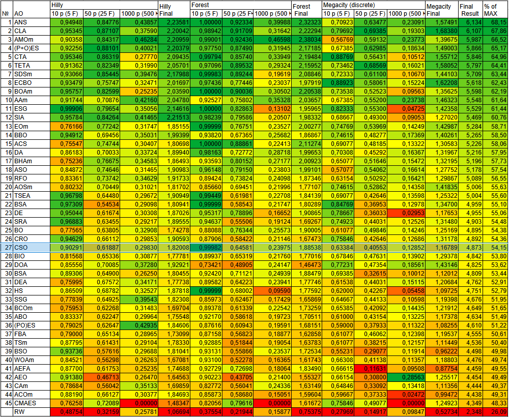
Figure 2. Color coding of algorithms by the corresponding tests

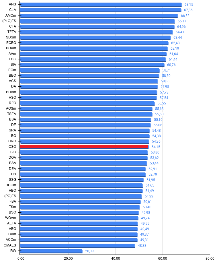
Figure 3. Histogram of the algorithm test results (on a scale from 0 to 100; the higher the score, the better, where 100 is the maximum possible theoretical result; the archive contains a script for calculating the ranking table)

Pros and Cons of the CSO Algorithm

Pros:

1. Only one additional parameter besides the population size.
2. A simple and straightforward concept.

Cons:

1. No significant drawbacks were identified.

An archive containing the latest versions of the algorithm code is attached to the article. The author of this article does not guarantee absolute accuracy in the descriptions of the canonical algorithms; many of them have been modified to improve their search capabilities. The conclusions and judgments presented in the articles are based on the results of the experiments conducted.

• GitHub: https://github.com/JQSakaJoo/Population-optimization-algorithms-MQL5

Files used in the article

#	Name	Type	Description
1	#C_AO.mqh	Include file	Parent class for population-based optimization algorithms
2	#C_AO_enum.mqh	Include file	Enumeration of population-based optimization algorithms
3	TestFunctions.mqh	Include file	Test function library
4	TestStandFunctions.mqh	Include file	Test bench function library
5	TestStand3D.mqh	Include file	3D visualization panel for the test bench
6	Utilities.mqh	Include file	Utility functions library
7	CalculationTestResults.mqh	Include file	Script for calculating results for a comparison table
8	Testing AOs.mq5	Script	Unified test bench for all population-based optimization algorithms
9	Simple Use of Population Optimization Algorithms.mq5	Script	Simple example of using population-based optimization algorithms without visualization
10	Test_CSO.mq5	Script	Test bench for CSO