

Swarm Optimizer with Hierarchical Sub-Flocks — Flock by Leader
 136
136
 0
0

Table of Contents
Introduction
If you are optimizing the parameters of a trading system or another high-dimensional model using swarm-based methods, you often face two conflicting problems: the population quickly “collapses” to a single point and stops exploration, while attempting to maintain diversity sharply increases computational costs and the spread of results. Given a fixed computational budget, it would be desirable for the algorithm to simultaneously: (1) intensively exploit promising areas — exploitation, (2) maintain several independent search “hotspots” — exploration, and (3) retain global exploration.
In this article, we examine whether the Flock by Leader (FBL) architecture solves this problem. The idea is simple and reproducible: the population is divided into sub-flocks based on density (ARF); within each sub-flock, a leader is assigned based on its personal best (fB); and different movement rules are defined for the three roles — leader, follower, and outlier. In this article, we formalize the ARF metric and the update rules, provide pseudocode, implement the C_AO_FBL component for MQL5, specify the control parameters (popSize, k, phi, wSep), and define clear success criteria: the quality of the solutions found, the stability of the results, and the computational cost within a given computational budget.
Algorithm Implementation
Watch a flock of starlings flying over the city. Hundreds of birds move as if they were a single organism — turning in unison, spreading out, and coming together again. At the same time, no one is giving orders; there is no central control. Each bird keeps track of only a few of its nearest neighbors, but the flock is not homogeneous: biologists have determined that there is a stable hierarchy within it. Some birds consistently fly in front and set the course, while others follow them.
This hierarchy is not set in stone — it shifts every minute depending on which bird is better able to navigate the current situation. It is precisely this principle that underlies the Flock by Leader algorithm. The population of optimization agents is divided into sub-flocks — small groups, each with its own internal hierarchy. Roles within the hierarchy are reassigned at every iteration: the leader is the agent that found the best solution in its group, not the one that simply happened to be at the geometric center. The rest follow the leader of their group, gradually converging toward good regions of the search space. Agents that are not assigned to any group carry out free exploration.
This division of labor solves the main problem with homogeneous swarm methods: when the entire population converges on a single point, it stops exploring the rest of the space. In FBL, several sub-flocks simultaneously exploit different promising regions, while outliers continuously check what has not yet been covered.
At the beginning of each iteration, the algorithm examines the current positions of all agents and asks: who is at the center of a dense cluster, and who is on the periphery or alone? To determine the answer, the ARF (Agent Role Factor) metric is calculated. The ARF concept is based on two sets for each agent. First, the direct neighborhood: all agents located within a radius of "d_max" from a given agent, where d_max is the distance to the k-th nearest neighbor. This is the agent's personal space — the agents it considers its neighbors. Second, the reverse neighborhood: all agents whose personal space this agent enters. These are the agents that consider it their neighbor.
ARF is the ratio of the size of the reverse neighborhood to the sum of both: ARF = |reverse neighborhood| / (|reverse neighborhood| + |direct neighborhood|).
Let's break down what this means in practice. If an agent is located at the center of a dense group, many agents around it include it in their personal space — the reverse neighborhood is large. At the same time, its own radius "d_max" is small because its "k" neighbors are very close by, and its direct neighborhood is not very large either. ARF approaches one. If an agent is located on the periphery or is completely alone, no other agent includes it in its personal space — the reverse neighborhood is small or empty. On the other hand, to find "k" neighbors, it has to reach far; its radius "d_max" is large, and its direct neighborhood is large. ARF approaches zero.
Agents with ARF >= 0.5 become centroids — the geometric centers of sub-flocks. If no agent has reached the threshold, the one with the highest ARF is selected. This serves as a safeguard for the first few iterations, when the agents are still evenly distributed. Each centroid attracts agents within its "d_max" radius. An agent that falls within the radius of several centroids is assigned to the one with the highest rank — a special numerical measure of the sub-flock's significance. The rank takes into account the density of the cluster: the more agents the centroid has gathered around itself, the higher its rank. The number of sub-flocks is capped: if there are too many centroids (when k is small), the excess ones with low ranks are discarded. This prevents the population from breaking up into dozens of tiny, ineffective groups. This raises a key question: which member of the sub-flock becomes its leader? It is precisely in answering this question that the algorithm makes a fundamental choice.
The centroid determines the geometry of the sub-flock — where it is located in space. But the centroid is not necessarily located at a good point in the landscape. Imagine this: a swarm has gathered on a hillside. The centroid — an agent located roughly in the middle of this group — is at an elevation of 650 meters. But one of the other members of the swarm reached an altitude of 820 meters and recorded that location as its personal best. It becomes the leader of the swarm — the one whose personal best "fB" is the best among all group members. The entire sub-flock will move toward that agent, rather than toward the geometric center.
Why is the personal best "fB" used instead of the current fitness value "f"? The current value is unreliable: the agent might have happened to end up in a good spot in this particular iteration, but its overall search history is weak. A personal best reflects the best place an agent has visited over the entire run of the algorithm — it is a stable quality signal.
The sub-flock leader is currently the best in its group. Its task is to continue improving the solution it has found while remaining a point of attraction for its followers. Three forces act on it. Inertia — it continues to move in the direction it was moving. A coefficient of 0.729 (the standard Clerc–Kennedy constriction coefficient) gradually dampens the velocity, preventing the leader from accelerating into chaotic wandering. Attraction to the personal best — the leader remembers the best place it has visited and is drawn to it. Attraction to the global best — the leader knows the best place in the entire population and is drawn to it with a force of "phi." These three forces are combined in a randomly weighted manner for each coordinate separately. The independence of the weights across coordinates is fundamentally important: the agent can move diagonally across the landscape, advancing vigorously along some axes and cautiously along others.
If an agent has just become a leader — having been a follower or an outlier in the previous iteration — its accumulated velocity is halved, but not reset to zero. A complete reset would be wasteful: some of the momentum it has built up is still useful. However, the previous direction was oriented toward another leader, so halving the velocity removes excess momentum without losing all the dynamics.
A follower is a member of a sub-flock that is not its leader. It moves along with the group, is drawn toward the leader, and at the same time preserves its own search history. Four forces, plus repulsion, act on it. Cohesion pulls it toward the leader's current position: "go to where the leader is." Alignment adjusts its velocity to the leader's velocity: "move in the direction the leader is moving." The cognitive component gravitates toward the best place it has found: "remember your discoveries." The global component attracts the agent toward the global best found by the entire population. Separation is the repulsive force away from neighbors that are too close; more on this below.
Let's look at an example. The leader of sub-flock "L" has found a good point on the landscape and is moving toward it with a velocity of (1.8, 0.7) along the two coordinates. Follower "F" is 12 units south of "L". Its personal best is a good point 5 units to the east. Cohesion pulls "F" northward (toward "L"). Alignment adds a component in the direction (1.8, 0.7) — the direction in which "L" is moving. The cognitive component adds an eastward offset. As a result, "F" moves northeast, maintaining both its course toward the leader and the memory of its own discovery.
An important technical detail in the alignment component. For velocity alignment, the leader's current velocity after its update in this iteration is not used; instead, a stored velocity value is used — the value from before the updates began. Leaders are updated first (Pass 1), and followers are updated second (Pass 2). If the follower uses the leader's already-adjusted velocity, it aligns itself with the "future" direction that the leader has not yet traveled. Using the saved velocity value makes the alignment physically correct: the agent aligns its motion with what the leader actually did, rather than with what the leader is about to do.
Without an additional mechanism, cohesion would eventually draw all members of the sub-flock toward a single point — the leader's position. Twenty agents in one place evaluating fitness twenty times at the same point — that is a complete waste of the computational budget. Separation — the repulsive force that prevents agents from sticking together. A discomfort zone is calculated for each agent: half the radius of its neighborhood "d_max". If a neighbor enters this zone, the agent receives a push away from it. The push force is greater the closer the neighbor is: at a distance equal to half of "d_max", the force is zero; when the positions coincide exactly, it is maximal. Result: The members of the sub-flock move toward the leader but maintain a healthy distance from one another. The swarm moves as a dense but not clumped-together group, covering the leader's neighborhood and exploring it more broadly.
The "separation" weight is specified by the "wSep" parameter. When "wSep" is large, the agents diverge significantly, and the sub-flocks are loose. When it is small, they are dense and at risk of collapsing.
An outlier is an agent that has ended up outside all swarms. It was not covered by the radius of any centroid. It is an isolated searcher with no group and no leader. Its behavior is simple. For each coordinate independently: with a 50% probability, it moves to the vicinity of the global best, adding a random offset within 20% of the range — this is a local search near the best-known point. With a 50% probability, it flies off to a completely random point within the search space — this is global diversification. It is precisely this coordinate-wise independence that makes the outlier's behavior so rich.
If the decision were made once for the entire agent, there would be only two possible patterns: either the entire agent jumps to "gBest", or it flies off entirely to a random location. With a coordinate-wise decision, a range of intermediate possibilities arises: some coordinates explore the neighborhood of "gBest", while others move to random locations. In a high-dimensional space, this fundamentally expands search coverage. After any jump, the agent's velocity is reset to zero — the accumulated inertia from the previous movement is irrelevant to the new random position. Consider the illustration below.
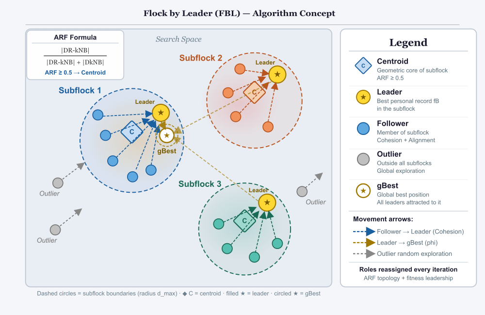
Figure 1. Illustration of the FBL algorithm in operation
The illustration on the left shows a search space with three colored sub-flocks (blue, orange, and green). Each swarm shows its complete structure: a dashed circle represents the swarm boundary (the centroid's "d_max" radius), a diamond with the letter C represents the centroid (an agent with ARF ≥ 0.5, the geometric core), a gold star represents the leader (the agent with the best "fB" in the group, which may not coincide with the centroid), and blue circles with arrows represent followers moving toward the leader. The gray circles outside all the swarms represent outliers with random exploration arrows. The white star in the ring is gBest, toward which all three leaders are pulled by gold arrows. The colored spots in the background hint at the topography of the fitness landscape. In the upper-left corner is the ARF formula with a threshold of 0.5. On the right side of the image is a legend explaining each symbol.
Let's move on to writing the pseudocode for the FBL algorithm.
FBL (Flock by Leader) pseudocode
Notations

    N — population size (popSize), D — dimensionality.
    kEff = min(k, N-1) — effective number of neighbours.
    x[i] — i agent's current position, v[i] — velocity.
    pBest[i] — personal best (position), fBest[i] — its fitness.
    gBest — global best (position).
    dist(i,j) — normalized distance between agents.
    dMax[i] — distance to kEff th nearest neighbour of i agent.
    Nout[i] — direct k-neighbourhood (who is considered neighbours by i), Nin[i] — reverse (who considers i to be its neighbour).
    ARF[i] = |Nin[i]| / (|Nin[i]| + |Nout[i]|).
    Roles: LEADER, FOLLOWER, OUTLIER.

Iteration t = 1..T
Step 0. Snapshots (for correct alignment)

    xSnap[i] ← x[i] for all i
    vSnap[i] ← v[i] for all i

Step 1. Distances and k-nearest neighbours

For each i agent:

    Compute dist(i,j) for all j ≠ i
    Sort j in ascending order dist(i,j)
    knnIdx[i] ← first kEff indices
    dMax[i] ← dist(i, knnIdx[i][kEff])
    Nout[i] ← { j | dist(i,j) ≤ dMax[i] } ("personal neighbourhood")

Step 2. Reverse neighbourhoods and ARF

    Reset Nin[i] (or |Nin[i]| counter) for all i
    For all (i, j) pairs, where j ∈ Nout[i]: add i to Nin[j]
    For each i:
    arf[i] ← |Nin[i]| / (|Nin[i]| + |Nout[i]|)

Step 3. Selecting centroids (sub-flock cores) and ranking

    centroids ← { i | arf[i] ≥ 0.5 }
    If 'centroids' is empty:
    centroids ← { argmax_i arf[i] } (a safeguard for early iterations)
    For each c centroid:
    Candidate sub-flock radius: R[c] ← dMax[c]
    rank[c] ← 0 (to be filled with the number of attached agents)
    If there are too many centroids (upper limit):
    leave centroids with the highest rank/density (accurate rule — like in the implementation)

Step 4. Assigning agents to sub-flocks and OUTLIER roles

    subflockId[i] ← -1 for all i
    For each i agent:
    Find the set of eligible centroids:
    C(i) = { c ∈ centroids | dist(i,c) ≤ R[c] }
    If C(i) is empty: role[i] ← OUTLIER, subflockId[i] ← -1
    Otherwise:
    select c* with maximum rank[c] (or another rule in case of a conflict)
    subflockId[i] ← id(c*), do not assign role[i] yet
    rank[c*]++

Step 5. Select a leader in each sub-flock (by personal best fBest)

For each s sub-flock:

    members(s) ← { i | subflockId[i] = s }
    leader[s] ← argmax_{i ∈ members(s)} fBest[i]
    For all i ∈ members(s):
    if i = leader[s]: role[i] ← LEADER
    otherwise role[i] ← FOLLOWER

Step 6. Update positions (3 different movement rules)
6A. Updating leaders (Pass 1)

For each i agent with role[i]=LEADER:

    If prevRole[i] ≠ LEADER: v[i] ← 0.5 * v[i]
    Update velocity (inertia + pBest + gBest):
    v[i] ← 0.729*v[i]
    v[i] ← v[i] + randVec()* (pBest[i] - xSnap[i])
    v[i] ← v[i] + phi*randVec()* (gBest - xSnap[i])
    x[i] ← xSnap[i] + v[i]

6B. Updating followers (Pass 2)

For each i agent with role[i]=FOLLOWER:

    L ← leader[subflockId[i]]
    Count sep ← Separation(i) (by knnIdx[i], zone 0.5*dMax[i], weight wSep)
    Update velocity (cohesion + alignment + pBest + gBest + separation):
    v[i] ← v[i] + wCoh*randVec()*(xSnap[L] - xSnap[i])
    v[i] ← v[i] + wAli*randVec()*(vSnap[L] - vSnap[i]) (note: take vSnap!)
    v[i] ← v[i] + wCog*randVec()*(pBest[i] - xSnap[i])
    v[i] ← v[i] + phi*wGlob*randVec()*(gBest - xSnap[i])
    v[i] ← v[i] + sep
    x[i] ← xSnap[i] + v[i]

6C. Updating outliers (OUTLIER)

For each i agent with role[i]=OUTLIER:

    For each coordinate d=1..D:
    if rand()<0.5:
    x[i][d] ← gBest[d] + uniform(-0.2*range[d], +0.2*range[d])
    otherwise:
    x[i][d] ← uniform(min[d], max[d])
    v[i] ← 0

Step 7. Bounds, evaluation, and record updates

    Limit x[i] in accessible range (clamp/repair)
    Calculate f[i] = Fitness(x[i])
    If f[i] > fBest[i]: update fBest[i], pBest[i]
    If f[i] > f(gBest): update gBest
    prevRole[i] ← role[i]
Now we can write the implementation.
The C_AO_FBL class implements the Flock by Leader algorithm as a standard component that inherits from the C_AO base class of the unified test bench. The inheritance architecture ensures compatibility with the testing infrastructure: the class provides the same three entry points (Init, Moving, Revision) and relies on the same "S_AlgoParam" parameter mechanism.
The algorithm is controlled by four external parameters. The "popSize" parameter specifies the population size and determines the ratio of the number of function evaluations to the number of iterations. The "k" parameter sets the number of nearest neighbors when constructing k-neighborhoods; it is the main regulator of the topological structure: a small "k" produces many small sub-flocks with active exploration, while a large "k" produces large, few sub-flocks with dominant exploitation. The recommended value for k is ≈ popSize × 0.1. The "phi" parameter determines the strength of attraction to the global best for both leaders and followers; when phi = 0, the sub-flocks operate independently, and when "phi" is large, the population collapses to a single point. The "wSep" parameter controls the weight of the "separation" vector and determines how strongly agents are repelled from overly close neighbors within a sub-flock.
The algorithm's internal state is stored in several groups of arrays. The "V" and "Vsnap" arrays store the agents' current velocities and the saved velocities recorded at the beginning of each iteration. The "cPsnap" array records the agents' positions before the updates begin. The "distM" matrix contains the normalized pairwise distances between all agents. The arrays "dMax," "dknbSz," "drknbSz," and "arf" store the neighborhood radii, the sizes of direct and reverse neighborhoods, and the "ARF" values for each agent. The "knnIdx" array stores the indices of the "k" nearest neighbors for each agent and is used when calculating "separation." The arrays "subflockId," "leaderIdx," "role," and "prevRole" encode the topological structure of the population and the role state of each agent. The arrays "centroidBuf," "subflockLeader," "subflockBestF," and "rankBuf" are working buffers used to construct the sub-flock hierarchy and sort the centroids.
//────────────────────────────────────────────────────────────────────
class C_AO_FBL : public C_AO
{
public: //------------------------------------------------------------
  ~C_AO_FBL () { }
  C_AO_FBL ()
  {
    ao_name = "FBL";
    ao_desc = "Flock by Leader";
    ao_link = "https://www.mql5.com/en/articles/21821";

    popSize = 50;
    k       = 5;
    phi     = 0.5;   // [F1]
    wSep    = 0.15;  // [F6]

    ArrayResize (params, 4);
    params [0].name = "popSize";
    params [0].val = popSize;
    params [1].name = "k";
    params [1].val = k;
    params [2].name = "phi";
    params [2].val = phi;
    params [3].name = "wSep";
    params [3].val = wSep;
  }

  void SetParams ()
  {
    popSize = (int)params [0].val;
    k       = (int)params [1].val;
    phi     =      params [2].val;
    wSep    =      params [3].val;
  }

  bool Init (const double &rangeMinP  [],
             const double &rangeMaxP  [],
             const double &rangeStepP [],
             const int     epochsP = 0);

  void Moving   ();
  void Revision ();

  //------------------------------------------------------------------
  int    k;    // k nearest neighbors for DkNB / DR-kNB / ARF
  double phi;  // attraction coefficient to gBest
  double wSep; // separation vector weight                                [F6]

private: //---------------------------------------------------------
  double V              []; // velocities [popSize * coords]
  double Vsnap          []; // velocity snapshot [popSize * coords] [F4]
  double Vmax           []; // velocity limit [coords]
  double cPsnap         []; // position snapshot       [popSize * coords]
  double sepVec         []; // separation vector     [coords]
  double distM          []; // normalized distance matrix [popSize × popSize]
  double dMax           []; // d_max^i               [popSize]
  int    dknbSz         []; // |DkNB_t(x_i)|         [popSize]
  int    drknbSz        []; // |DR-kNB_t(x_i)|       [popSize]
  double arf            []; // ARF_t(A_i)             [popSize]
  int    knnIdx         []; // k-NN indices           [popSize * kEff]
  int    subflockId     []; // agent sub-flock (-1 = outlier) [popSize]
  int    leaderIdx      []; // sub-flock leader index [popSize]
  int    role           []; // 0=leader, 1=follower 2 = outlier [popSize]
  int    prevRole       []; // role from the previous iteration [popSize]
  int    centroidBuf    []; // centroids, sorted by ARF↓ [popSize]
  int    subflockLeader []; // leader of sub-flock s [popSize]
  double subflockBestF  []; // best fB in sub-flock s [popSize]
  double rankBuf        []; // Rank_t(A_i) Formula 5  [popSize]          [F7]
  double tmpDist        []; // k-NN sorting buffer  [popSize]
  int    tmpIdx_        []; // k-NN index buffer    [popSize]
  int    kEff;              // min(k, popSize - 1)
  int    nCentroids;        // number of sub-flocks per iteration

  int    Idx   (int i, int c)
  {
    return i * coords + c;
  }
  double Clamp (double v, double lo, double hi)
  {
    return v < lo ? lo : v > hi ? hi : v;
  }

  void   CalcSep (int i); // Calculate sepVec[] for agent i
};
//————————————————————————————————————————————————————————————————————
The Init method performs one-time initialization before optimization begins. It calls the standard initializer of the base class, StandardInit, which allocates the agent arrays and copies the search ranges. Next, the effective number of neighbors, kEff = min(k, popSize − 1), is calculated — a safeguard against invalid values of the “k” parameter. All internal arrays are allocated based on the population size and the number of coordinates. "Vmax" is set for each coordinate to half the range of that axis, which limits the agent's maximum step size per iteration. The agents' initial positions are set randomly and uniformly within the valid search space; their velocities are set to zero, and their personal bests are initialized to −DBL_MAX. All agents are assigned the follower role (role = 1), and the sub-flock counter is reset to zero.
//————————————————————————————————————————————————————————————————————
bool C_AO_FBL::Init (const double &rangeMinP  [],
                     const double &rangeMaxP  [],
                     const double &rangeStepP [],
                     const int     epochsP = 0)
{
  if (!StandardInit (rangeMinP, rangeMaxP, rangeStepP)) return false;

  kEff = MathMin (k, popSize - 1);
  if (kEff < 1) kEff = 1;

  ArrayResize (V,              popSize * coords);
  ArrayResize (Vsnap,          popSize * coords);  // [F4]
  ArrayResize (Vmax,           coords);
  ArrayResize (cPsnap,         popSize * coords);
  ArrayResize (sepVec,         coords);
  ArrayResize (distM,          popSize * popSize);
  ArrayResize (dMax,           popSize);
  ArrayResize (dknbSz,         popSize);
  ArrayResize (drknbSz,        popSize);
  ArrayResize (arf,            popSize);
  ArrayResize (knnIdx,         popSize * kEff);
  ArrayResize (subflockId,     popSize);
  ArrayResize (leaderIdx,      popSize);
  ArrayResize (role,           popSize);
  ArrayResize (prevRole,       popSize);
  ArrayResize (centroidBuf,    popSize);
  ArrayResize (subflockLeader, popSize);
  ArrayResize (subflockBestF,  popSize);
  ArrayResize (rankBuf,        popSize);
  ArrayResize (tmpDist,        popSize);
  ArrayResize (tmpIdx_,        popSize);

  for (int c = 0; c < coords; c++)
    Vmax [c] = (rangeMax [c] - rangeMin [c]) * 0.5;

  for (int i = 0; i < popSize; i++)
  {
    for (int c = 0; c < coords; c++)
    {
      a [i].cP [c]    = u.RNDfromCI (rangeMin [c], rangeMax [c]);
      V    [Idx (i, c)] = 0.0;
      Vsnap[Idx (i, c)] = 0.0;  // [F4]
    }
    a [i].fB    = -DBL_MAX;
    role     [i] = 1;
    prevRole [i] = 1;
    leaderIdx[i] = -1;
  }
  nCentroids = 0;
  return true;
}
//————————————————————————————————————————————————————————————————————
The Moving method performs a single operation: it copies the continuous working positions "cP" into the discretized positions "c" using the SeInDiSp function. It is the "c" coordinates that are passed to the external code to calculate the value of the fitness function. The distinction between "cP" and "c" allows the algorithm to operate in an internal continuous space (where the velocity equations yield fractional values) regardless of whether the actual problem is discrete or continuous — discretization occurs only when the fitness is queried.
//————————————————————————————————————————————————————————————————————
void C_AO_FBL::Moving ()
{
  for (int i = 0; i < popSize; i++)
    for (int c = 0; c < coords; c++)
      a [i].c [c] = u.SeInDiSp (a [i].cP [c], rangeMin [c], rangeMax [c], rangeStep [c]);
}
//————————————————————————————————————————————————————————————————————
The CalcSep method calculates the "separation" vector for agent "i" and writes it to the shared buffer "sepVec". The method implements Reynolds' first rule: an agent must maintain a minimum distance from its nearest neighbors.
The "separation" zone is defined as half the radius of the neighborhood: dSep = 0.5 × dMax[i]. The method iterates through all "kEff" nearest neighbors of agent "i," which were identified in advance in step 3 of the "Revision" method and stored in "knnIdx." If neighbor "j" is closer than "dSep," it contributes to the repulsion vector with a weight that is inversely proportional to the distance: the closer the neighbor, the stronger the repulsion. The weight is calculated as (dSep − dist) / dSep, which yields a value ranging from 0 at the zone boundary to 1 when the positions coincide. The resulting vector is scaled by the "wSep" parameter. Since the "cPsnap" position differences are expressed in absolute units of the search space, and "Vmax" is also specified in absolute units, the "sep" vector is directly comparable to the other velocity components.
//————————————————————————————————————————————————————————————————————
// [O2][F6] Separation vector for agent i → sepVec[].
// Repulsion from k-NN neighbors closer than dSep = 0.5 * dMax[i].
// sepVec[] in absolute position units; the scale is specified by wSep.
void C_AO_FBL::CalcSep (int i)
{
  ArrayInitialize (sepVec, 0.0);
  double dSep = 0.5 * dMax [i];
  if (dSep < 1e-14) return;

  for (int m = 0; m < kEff; m++)
  {
    int    j     = knnIdx [i * kEff + m];
    double normD = distM  [i * popSize + j];
    if (normD >= dSep) continue;
    double w = (normD > 1e-12) ? (dSep - normD) / dSep : 1.0;
    for (int c = 0; c < coords; c++)
      sepVec [c] += w * (cPsnap [Idx (i, c)] - cPsnap [Idx (j, c)]);
  }
  for (int c = 0; c < coords; c++) sepVec [c] *= wSep;  // [F6]
}
//————————————————————————————————————————————————————————————————————
The Revision method contains all the logic of the algorithm and is divided into 14 steps. It is called after the external code has filled in the a[i].f field for all agents based on the results of the "Moving" and "CalcFunc" calls.
Step 1 updates the personal best fB/cB values and the global best fB/cB. A personal best tracks the best position an agent has ever visited and is used in the cognitive component of the velocity formulas and — crucially — for selecting the leader of the sub-flock. The comparison is based on the discretized coordinates "c," not "cP," since it is "c" that was evaluated by the function.
Steps 2–5 form a topological picture of the population. The distance matrix is constructed by normalizing each axis to its respective range, which ensures that all coordinates contribute equally, regardless of their scale. This is critical for problems involving several hundred coordinates, where the axes may have fundamentally different ranges. Partial sorting by selection to find the "kEff" nearest neighbors runs in O(kEff × n) instead of O(n × log n) for a full sort — when kEff << n, this results in a significant time saving. "ARF" is calculated exactly according to formula 4 in the original article.
Step 6 selects the centroids and sorts them using the rank formula 5 from the article, adapted for optimization. The rank takes into account only the number of neighbors (topological weight), not fitness — this is intentional, since the rank determines priority in the event of a membership conflict between two sub-flocks, rather than leader selection. Limiting the number of centroids to popSize / kEff prevents fragmentation: when "k" is small, there is no point in having more sub-flocks than the connectivity of the k-NN graph allows.
Step 7 assigns agents to sub-flocks using the “first covering centroid” principle in descending order of rank: the more significant sub-flock captures boundary agents first. An agent outside all radii becomes an outlier.
Step 8 selects the leader of each sub-flock based on the best personal best "fB" among all members. Using "fB" instead of the current "f" makes the selection robust to noise: a weak agent with a randomly good current value will not become the leader if its historical best is weaker. The fallback for the first iteration (when fB = −DBL_MAX for everyone) designates the sub-flock's centroid as the leader.
Step 10 takes snapshots of "cPsnap" and "Vsnap" before any updates. A snapshot of positions is necessary to eliminate "ordering bias": all cohesion and "separation" components are calculated relative to stable old positions, rather than positions that gradually change during a single pass through the loop. The "Vsnap" velocity snapshot is necessary for "Alignment" to work correctly among followers: they align with the leader's velocity vector as it existed before the start of the iteration, rather than with the one that has already been modified in Pass 1. This makes the alignment physically meaningful: the agent aligns its direction with the leader's actual movement, rather than with the newly calculated momentum.
Pass 1 (Step 11) updates the leaders first. The Clerc–Kennedy constriction coefficient of 0.729 in the inertia component ensures guaranteed convergence of velocities for any values of "r1" and "r2" without the need to manually tune the inertia coefficient. When switching roles from follower to leader, the previous velocity is halved rather than completely reset to zero: the direction of the accumulated momentum is preserved, but its magnitude is reduced to a safe level.
Pass 2 (Step 12) updates the followers using the leaders' updated positions, "cPsnap" (a snapshot taken before the changes), and the old velocities, "Vsnap". The four velocity components correspond to the four forces acting on a follower: cohesion pulls it toward the sub-flock leader, "alignment" aligns the direction of movement, the cognitive component maintains a connection to the agent’s personal best, and the global component ensures slow convergence of the entire population toward the best solution found.
Pass 3 (Step 13) updates the outliers. An outlier is an agent that has ended up outside all swarms. In multidimensional space, the decision to jump is made independently for each coordinate: this allows the agent to move diagonally through the space, changing some coordinates within the "gBest" neighborhood and others randomly. This coordinate-wise decision provides a much greater variety of search patterns than a single decision for the agent as a whole.
//————————————————————————————————————————————————————————————————————
void C_AO_FBL::Revision ()
{
  //─── 1. Personal Bests and Global Best ───────────────────────────────
  for (int i = 0; i < popSize; i++)
  {
    if (a [i].f > a [i].fB)
    {
      a [i].fB = a [i].f;
      ArrayCopy (a [i].cB, a [i].c, 0, 0, coords);
    }
    if (a [i].f > fB)
    {
      fB       = a [i].f;
      ArrayCopy (cB,       a [i].c, 0, 0, coords);
    }
  }

  //─── 2. Normalized Distance Matrix ─────────────────────────
  for (int i = 0; i < popSize; i++)
  {
    distM [i * popSize + i] = 0.0;
    for (int j = i + 1; j < popSize; j++)
    {
      double d = 0.0;
      for (int c = 0; c < coords; c++)
      {
        double rng = rangeMax [c] - rangeMin [c];
        double df  = (rng > 0.0) ? (a [i].cP [c] - a [j].cP [c]) / rng : 0.0;
        d += df * df;
      }
      d = MathSqrt (d);
      distM [i * popSize + j] = d;
      distM [j * popSize + i] = d;
    }
  }

  //─── 3. k-NN → d_max → |DkNB| (Def. 5, Formula 3) ───────────────
  for (int i = 0; i < popSize; i++)
  {
    int cnt = 0;
    for (int j = 0; j < popSize; j++)
    {
      if (j == i) continue;
      tmpDist [cnt] = distM [i * popSize + j];
      tmpIdx_ [cnt] = j;
      cnt++;
    }
    for (int m = 0; m < kEff; m++)
    {
      int minPos = m;
      for (int n = m + 1; n < cnt; n++)
        if (tmpDist [n] < tmpDist [minPos]) minPos = n;
      if (minPos != m)
      {
        double td = tmpDist [m];
        tmpDist [m] = tmpDist [minPos];
        tmpDist [minPos] = td;
        int    ti = tmpIdx_ [m];
        tmpIdx_ [m] = tmpIdx_ [minPos];
        tmpIdx_ [minPos] = ti;
      }
    }
    dMax [i] = tmpDist [kEff - 1];
    for (int m = 0; m < kEff; m++) knnIdx [i * kEff + m] = tmpIdx_ [m];

    dknbSz [i] = 0;
    for (int j = 0; j < popSize; j++)
    {
      if (j == i) continue;
      if (distM [i * popSize + j] <= dMax [i]) dknbSz [i]++;
    }
  }

  //─── 4. |DR-kNB| (Definition 6) ─────────────────────────────────
  ArrayInitialize (drknbSz, 0);
  for (int i = 0; i < popSize; i++)
    for (int j = 0; j < popSize; j++)
    {
      if (j == i) continue;
      if (distM [i * popSize + j] <= dMax [j]) drknbSz [i]++;
    }

  //─── 5. ARF (Formula 4) ──────────────────────────────────────────
  for (int i = 0; i < popSize; i++)
  {
    int denom = drknbSz [i] + dknbSz [i];
    arf [i] = (denom > 0) ? (double)drknbSz [i] / (double)denom : 0.5;
  }

  //─── 6. Centroids: ARF >= 0.5, sorted by Rank↓ (Formula 5) ──
  nCentroids = 0;
  for (int i = 0; i < popSize; i++)
    if (arf [i] >= 0.5) centroidBuf [nCentroids++] = i;

  if (nCentroids == 0)
  {
    int bestI = 0;
    for (int i = 1; i < popSize; i++) if (arf [i] > arf [bestI]) bestI = i;
    centroidBuf [0] = bestI;
    nCentroids = 1;
  }

  // [F7] Formula 5: Rank_t(A_i) = Log(|N_i,t| / |N_t| * 10) * ARF_t(A_i)
  // |N_i,t| = dknbSz[i] (the number of neighbors of agent i)
  // |N_t|   = popSize   (the total number of agents)
  // The Log argument is protected against zero: if dknbSz == 0, then rank = 0.
  for (int i = 0; i < popSize; i++)
  {
    double ratio = (double)dknbSz [i] / (double)popSize * 10.0;
    rankBuf [i]  = (ratio > 1e-12) ? MathLog (ratio) * arf [i] : 0.0;
  }

  // Insertion sort of centroids by Rank↓
  for (int a_ = 1; a_ < nCentroids; a_++)
  {
    int    key  = centroidBuf [a_];
    double keyR = rankBuf [key];
    int    b_   = a_ - 1;
    while (b_ >= 0 && rankBuf [centroidBuf [b_]] < keyR)
    {
      centroidBuf [b_ + 1] = centroidBuf [b_];
      b_--;
    }
    centroidBuf [b_ + 1] = key;
  }

  // [F9] Pruning: keep no more than popSize/k centroids.
  // Sorting has already been performed → the most significant leaders are at the beginning of the array.
  int maxCentroids = MathMax (1, popSize / kEff);
  if (nCentroids > maxCentroids) nCentroids = maxCentroids;

  //─── 7. Assigning agents to sub-flocks ────────────────────────────
  for (int i = 0; i < popSize; i++) subflockId [i] = -1;

  for (int s = 0; s < nCentroids; s++)
    subflockId [centroidBuf [s]] = s;

  for (int i = 0; i < popSize; i++)
  {
    if (subflockId [i] >= 0) continue;
    for (int s = 0; s < nCentroids; s++)
    {
      if (distM [i * popSize + centroidBuf [s]] <= dMax [centroidBuf [s]])
      {
        subflockId [i] = s;
        break;
      }
    }
  }

  //─── 8. Sub-flock leader = the agent with the best fB in the sub-flock ─────────
  // [F2] We use fB (historical best) rather than f (current, noisy).
  for (int s = 0; s < nCentroids; s++)
  {
    subflockLeader [s] = -1;
    subflockBestF  [s] = -DBL_MAX;
  }
  for (int i = 0; i < popSize; i++)
  {
    int s = subflockId [i];
    if (s < 0) continue;
    if (a [i].fB > subflockBestF [s])  // [F2] fB instead of f
    {
      subflockBestF  [s] = a [i].fB;
      subflockLeader [s] = i;
    }
  }

  // Fallback: if no agent in the sub-flock had fB > -DBL_MAX
  // (for example, on the first iteration), designate the centroid as the leader,
  // so that the followers' leaderIdx is never -1.
  for (int s = 0; s < nCentroids; s++)
    if (subflockLeader [s] < 0) subflockLeader [s] = centroidBuf [s];

  //─── 9. Agent roles ─────────────────────────────────────────────
  for (int i = 0; i < popSize; i++)
  {
    int s = subflockId [i];
    if      (s < 0)
    {
      role      [i] = 2;
      leaderIdx [i] = -1;
    }
    else if (subflockLeader [s] == i)
    {
      role      [i] = 0;
      leaderIdx [i] = -1;
    }
    else
    {
      role      [i] = 1;
      leaderIdx [i] = subflockLeader [s];
    }
  }

  //─── 10. Snapshots of positions and velocities before the update ──────────
  // [F4] Vsnap is taken here — Pass 2 uses consistent
  //      old leader velocities, not those already changed in Pass 1.
  for (int i = 0; i < popSize; i++)
    for (int c = 0; c < coords; c++)
    {
      cPsnap [Idx (i, c)] = a [i].cP [c];
      Vsnap  [Idx (i, c)] = V  [Idx (i, c)];  // [F4]
    }

  //─── 11. Pass 1: LEADERS ──────────────────────────────────────────
  // v = w·v + r1·(cB_i − cP_i) + φ·r2·(gBest − cP_i) + sep
  // [F10] w=0.729 — Clerc–Kennedy constriction coefficient (fixed).
  for (int i = 0; i < popSize; i++)
  {
    if (role [i] != 0) continue;

    // [F3] Soft velocity reset when first appearing in the leader role.
    //      The accumulated momentum is halved rather than reset to zero.
    if (prevRole [i] != 0)
      for (int c = 0; c < coords; c++) V [Idx (i, c)] *= 0.5;  // [F3]

    CalcSep (i);

    for (int c = 0; c < coords; c++)
    {
      double r1   = u.RNDfromCI (0.0, 1.0);
      double r2   = u.RNDfromCI (0.0, 1.0);
      int    idx  = Idx (i, c);
      double vNew = 0.729 * V [idx]                              // [F10] inertia
                    + r1 * (a [i].cB [c] - cPsnap [idx])         // cognitive
                    + phi * r2 * (cB [c]  - cPsnap [idx])        // global
                    + sepVec [c];                                // separation

      vNew         = Clamp (vNew, -Vmax [c], Vmax [c]);
      a [i].cP [c] = Clamp (cPsnap [idx] + vNew, rangeMin [c], rangeMax [c]);
      V [idx]      = vNew;
    }
  }

  //─── 12. Pass 2: FOLLOWERS ───────────────────────────────────
  // v = w·v + r1·(cP_L − cP_i) + r2·(Vsnap_L − Vsnap_i)
  //       + r3·(cB_i − cP_i) + φ·r4·(gBest − cP_i) + sep
  // [F4] Alignment is based on the leader's Vsnap (previous velocity).
  // [F10] w=0.729 — Clerc–Kennedy constriction coefficient (fixed).
  for (int i = 0; i < popSize; i++)
  {
    if (role [i] != 1) continue;
    int wi = leaderIdx [i];

    CalcSep (i);

    for (int c = 0; c < coords; c++)
    {
      double r1   = u.RNDfromCI (0.0, 1.0);
      double r2   = u.RNDfromCI (0.0, 1.0);
      double r3   = u.RNDfromCI (0.0, 1.0);
      double r4   = u.RNDfromCI (0.0, 1.0);
      int    idx  = Idx (i, c);
      int    idxL = Idx (wi, c);
      double vNew = 0.729 * V [idx]                             // [F10] inertia
                    + r1 * (cPsnap [idxL] - cPsnap [idx])       // Cohesion
                    + r2 * (Vsnap  [idxL] - Vsnap  [idx])       // Alignment [F4]
                    + r3 * (a [i].cB [c]  - cPsnap [idx])       // Cognitive
                    + phi * r4 * (cB [c]  - cPsnap [idx])       // Global
                    + sepVec [c];                               // Separation

      vNew         = Clamp (vNew, -Vmax [c], Vmax [c]);
      a [i].cP [c] = Clamp (cPsnap [idx] + vNew, rangeMin [c], rangeMax [c]);
      V [idx]      = vNew;
    }
  }

  //─── 13. Pass 3: OUTLIERS ─────────────────────────────────────────
  // [F5] r is independent for each coordinate—in a multidimensional
  //      space, the coordinates jump independently.
  for (int i = 0; i < popSize; i++)
  {
    if (role [i] != 2) continue;

    for (int c = 0; c < coords; c++)
    {
      double r    = u.RNDfromCI (0.0, 1.0);  // [F5] per-coordinate
      double xNew = (r > 0.5)
                    ? cB [c] + u.RNDfromCI (-1.0, 1.0) * (rangeMax [c] - rangeMin [c]) * 0.2
                    : u.RNDfromCI (rangeMin [c], rangeMax [c]);

      a [i].cP [c]   = Clamp (xNew, rangeMin [c], rangeMax [c]);
      V [Idx (i, c)] = 0.0;
    }
  }

  //─── 14. Preserving Roles ────────────────────────────────────────
  for (int i = 0; i < popSize; i++) prevRole [i] = role [i];
}
//————————————————————————————————————————————————————————————————————
Test Results
The algorithm was tested on three standard test-bench functions — Hilly, Forest, and Megacity — at three levels of dimensionality: 10, 50, and 1000 coordinates, respectively, with 10,000 evaluations per run and 10 repetitions. This is an honest and straightforward answer to the original question: in its current form, the algorithm is not a ready-made tool for complex trading-system parameter selection tasks.FBL|Flock by Leader|50.0|10.0|0.5|0.9|
=============================
5 Hilly's; Func runs: 10000; result: 0.6316210581453732
25 Hilly's; Func runs: 10000; result: 0.45555817277200505
500 Hilly's; Func runs: 10000; result: 0.2640456113290198
=============================
5 Forest's; Func runs: 10000; result: 0.6112393067788322
25 Forest's; Func runs: 10000; result: 0.4289609729927785
500 Forest's; Func runs: 10000; result: 0.1977883253085394
=============================
5 Megacity's; Func runs: 10000; result: 0.46153846153846156
25 Megacity's; Func runs: 10000; result: 0.2827692307692308
500 Megacity's; Func runs: 10000; result: 0.10590769230769326
=============================
Overall score: 3.43943 (38.22%)
Below is a visualization of the algorithm operating on test functions: both those used to calculate the ranking and standard research functions. The 3D visualization panel for the test bench has been redesigned and rewritten. You can now see the functions in motion and evaluate the algorithm's performance even more clearly.

FBL on the Hilly test function

FBL on the Forest test function

FBL on the Megacity test function

FBL on the Paraboloid test function

FBL on the GoldsteinPrice test function
With an overall score of 38.22%, FBL does not make the list of the top 45 optimization methods on our test bench. This is an honest and unequivocal answer to the original question: as it stands, the algorithm is not a ready-to-use tool for complex tasks of tuning trading system parameters. The FBL algorithm is presented in the ranking table for informational purposes only.
| No. | AO | Description | Hilly | Hilly Final | Forest | Forest Final | Megacity (discrete) | Megacity Final | Final Result | % of MAX | ||||||
| 10 p (5 F) | 50 p (25 F) | 1000 p (500 F) | 10 p (5 F) | 50 p (25 F) | 1000 p (500 F) | 10 p (5 F) | 50 p (25 F) | 1000 p (500 F) | ||||||||
| 1 | ANS | across neighbourhood search | 0.94948 | 0.84776 | 0.43857 | 2.23581 | 1.00000 | 0.92334 | 0.39988 | 2.32323 | 0.70923 | 0.63477 | 0.23091 | 1.57491 | 6.134 | 68.15 |
| 2 | CLA | code lock algorithm (joo) | 0.95345 | 0.87107 | 0.37590 | 2.20042 | 0.98942 | 0.91709 | 0.31642 | 2.22294 | 0.79692 | 0.69385 | 0.19303 | 1.68380 | 6.107 | 67.86 |
| 3 | AMOm | animal migration optimization M | 0.90358 | 0.84317 | 0.46284 | 2.20959 | 0.99001 | 0.92436 | 0.46598 | 2.38034 | 0.56769 | 0.59132 | 0.23773 | 1.39675 | 5.987 | 66.52 |
| 4 | (P+O)ES | (P+O) evolution strategies | 0.92256 | 0.88101 | 0.40021 | 2.20379 | 0.97750 | 0.87490 | 0.31945 | 2.17185 | 0.67385 | 0.62985 | 0.18634 | 1.49003 | 5.866 | 65.17 |
| 5 | CTA | comet tail algorithm (joo) | 0.95346 | 0.86319 | 0.27770 | 2.09435 | 0.99794 | 0.85740 | 0.33949 | 2.19484 | 0.88769 | 0.56431 | 0.10512 | 1.55712 | 5.846 | 64.96 |
| 6 | TETA | time evolution travel algorithm (joo) | 0.91362 | 0.82349 | 0.31990 | 2.05701 | 0.97096 | 0.89532 | 0.29324 | 2.15952 | 0.73462 | 0.68569 | 0.16021 | 1.58052 | 5.797 | 64.41 |
| 7 | SDSm | stochastic diffusion search M | 0.93066 | 0.85445 | 0.39476 | 2.17988 | 0.99983 | 0.89244 | 0.19619 | 2.08846 | 0.72333 | 0.61100 | 0.10670 | 1.44103 | 5.709 | 63.44 |
| 8 | ECBO | enhanced_colliding_bodies_optimization | 0.93479 | 0.75747 | 0.32471 | 2.01697 | 0.97436 | 0.77446 | 0.23037 | 1.97919 | 0.88923 | 0.58061 | 0.15224 | 1.62208 | 5.618 | 62.43 |
| 9 | BOAm | billiards optimization algorithm M | 0.95757 | 0.82599 | 0.25235 | 2.03590 | 1.00000 | 0.90036 | 0.30502 | 2.20538 | 0.73538 | 0.52523 | 0.09563 | 1.35625 | 5.598 | 62.19 |
| 10 | AAm | archery algorithm M | 0.91744 | 0.70876 | 0.42160 | 2.04780 | 0.92527 | 0.75802 | 0.35328 | 2.03657 | 0.67385 | 0.55200 | 0.23738 | 1.46323 | 5.548 | 61.64 |
| 11 | ESG | evolution of social groups (joo) | 0.99906 | 0.79654 | 0.35056 | 2.14616 | 1.00000 | 0.82863 | 0.13102 | 1.95965 | 0.82333 | 0.55300 | 0.04725 | 1.42358 | 5.529 | 61.44 |
| 12 | SIA | simulated isotropic annealing (joo) | 0.95784 | 0.84264 | 0.41465 | 2.21513 | 0.98239 | 0.79586 | 0.20507 | 1.98332 | 0.68667 | 0.49300 | 0.09053 | 1.27020 | 5.469 | 60.76 |
| 13 | EOm | extremal_optimization_M | 0.76166 | 0.77242 | 0.31747 | 1.85155 | 0.99999 | 0.76751 | 0.23527 | 2.00277 | 0.74769 | 0.53969 | 0.14249 | 1.42987 | 5.284 | 58.71 |
| 14 | BBO | biogeography-based optimization | 0.94912 | 0.69456 | 0.35031 | 1.99399 | 0.93820 | 0.67365 | 0.25682 | 1.86867 | 0.74615 | 0.48277 | 0.17369 | 1.40261 | 5.265 | 58.50 |
| 15 | ACS | artificial cooperative search | 0.75547 | 0.74744 | 0.30407 | 1.80698 | 1.00000 | 0.88861 | 0.22413 | 2.11274 | 0.69077 | 0.48185 | 0.13322 | 1.30583 | 5.226 | 58.06 |
| 16 | DA | dialectical algorithm | 0.86183 | 0.70033 | 0.33724 | 1.89940 | 0.98163 | 0.72772 | 0.28718 | 1.99653 | 0.70308 | 0.45292 | 0.16367 | 1.31967 | 5.216 | 57.95 |
| 17 | BHAm | Black Hole Algorithm M | 0.75236 | 0.76675 | 0.34583 | 1.86493 | 0.93593 | 0.80152 | 0.27177 | 2.00923 | 0.65077 | 0.51646 | 0.15472 | 1.32195 | 5.196 | 57.73 |
| 18 | ASO | anarchy society optimization | 0.84872 | 0.74646 | 0.31465 | 1.90983 | 0.96148 | 0.79150 | 0.23803 | 1.99101 | 0.57077 | 0.54062 | 0.16614 | 1.27752 | 5.178 | 57.54 |
| 19 | RFO | royal flush optimization (JOO) | 0.83361 | 0.73742 | 0.34629 | 1.91733 | 0.89424 | 0.73824 | 0.24098 | 1.87346 | 0.63154 | 0.50292 | 0.16421 | 1.29867 | 5.089 | 56.55 |
| 20 | AOSm | atomic orbital search M | 0.80232 | 0.70449 | 0.31021 | 1.81702 | 0.85660 | 0.69451 | 0.21996 | 1.77107 | 0.74615 | 0.52862 | 0.14358 | 1.41835 | 5.006 | 55.63 |
| 21 | TSEA | turtle shell evolution algorithm (JOO) | 0.96798 | 0.64480 | 0.29672 | 1.90949 | 0.99449 | 0.61981 | 0.22708 | 1.84139 | 0.69077 | 0.42646 | 0.13598 | 1.25322 | 5.004 | 55.60 |
| 22 | BSA | backtracking_search_algorithm | 0.97309 | 0.54534 | 0.29098 | 1.80941 | 0.99999 | 0.58543 | 0.21747 | 1.80289 | 0.84769 | 0.36953 | 0.12978 | 1.34700 | 4.959 | 55.10 |
| 23 | DE | differential evolution | 0.95044 | 0.61674 | 0.30308 | 1.87026 | 0.95317 | 0.78896 | 0.16652 | 1.90865 | 0.78667 | 0.36033 | 0.02953 | 1.17653 | 4.955 | 55.06 |
| 24 | SRA | successful restaurateur algorithm (JOO) | 0.96883 | 0.63455 | 0.29217 | 1.89555 | 0.94637 | 0.55506 | 0.19124 | 1.69267 | 0.74923 | 0.44031 | 0.12526 | 1.31480 | 4.903 | 54.48 |
| 25 | BO | bonobo_optimizer | 0.77565 | 0.63805 | 0.32908 | 1.74278 | 0.88088 | 0.76344 | 0.25573 | 1.90005 | 0.61077 | 0.49846 | 0.14246 | 1.25169 | 4.895 | 54.38 |
| 26 | CRO | chemical reaction optimization | 0.94629 | 0.66112 | 0.29853 | 1.90593 | 0.87906 | 0.58422 | 0.21146 | 1.67473 | 0.75846 | 0.42646 | 0.12686 | 1.31178 | 4.892 | 54.36 |
| 27 | CSO | competitive_swarm_optimizer | 0.90291 | 0.61887 | 0.29830 | 1.82008 | 0.99982 | 0.64581 | 0.23975 | 1.88538 | 0.63384 | 0.40553 | 0.12852 | 1.16789 | 4.873 | 54.15 |
| 28 | BIO | blood inheritance optimization (JOO) | 0.81568 | 0.65336 | 0.30877 | 1.77781 | 0.89937 | 0.65319 | 0.21760 | 1.77016 | 0.67846 | 0.47631 | 0.13902 | 1.29378 | 4.842 | 53.80 |
| 29 | DOA | dream_optimization_algorithm | 0.85556 | 0.70085 | 0.37280 | 1.92921 | 0.73421 | 0.48905 | 0.24147 | 1.46473 | 0.77231 | 0.47354 | 0.18561 | 1.43146 | 4.825 | 53.62 |
| 30 | BSA | bird swarm algorithm | 0.89306 | 0.64900 | 0.26250 | 1.80455 | 0.92420 | 0.71121 | 0.24939 | 1.88479 | 0.69385 | 0.32615 | 0.10012 | 1.12012 | 4.809 | 53.44 |
| 31 | DEA | dolphin_echolocation_algorithm | 0.75995 | 0.67572 | 0.34171 | 1.77738 | 0.89582 | 0.64223 | 0.23941 | 1.77746 | 0.61538 | 0.44031 | 0.15115 | 1.20684 | 4.762 | 52.91 |
| 32 | HS | harmony search | 0.86509 | 0.68782 | 0.32527 | 1.87818 | 0.99999 | 0.68002 | 0.09590 | 1.77592 | 0.62000 | 0.42267 | 0.05458 | 1.09725 | 4.751 | 52.79 |
| 33 | SSG | saplings sowing and growing | 0.77839 | 0.64925 | 0.39543 | 1.82308 | 0.85973 | 0.62467 | 0.17429 | 1.65869 | 0.64667 | 0.44133 | 0.10598 | 1.19398 | 4.676 | 51.95 |
| 34 | BCOm | bacterial chemotaxis optimization M | 0.75953 | 0.62268 | 0.31483 | 1.69704 | 0.89378 | 0.61339 | 0.22542 | 1.73259 | 0.65385 | 0.42092 | 0.14435 | 1.21912 | 4.649 | 51.65 |
| 35 | ABO | african buffalo optimization | 0.83337 | 0.62247 | 0.29964 | 1.75548 | 0.92170 | 0.58618 | 0.19723 | 1.70511 | 0.61000 | 0.43154 | 0.13225 | 1.17378 | 4.634 | 51.49 |
| 36 | (PO)ES | (PO) evolution strategies | 0.79025 | 0.62647 | 0.42935 | 1.84606 | 0.87616 | 0.60943 | 0.19591 | 1.68151 | 0.59000 | 0.37933 | 0.11322 | 1.08255 | 4.610 | 51.22 |
| 37 | FBA | fractal-based algorithm | 0.79000 | 0.65134 | 0.28965 | 1.73099 | 0.87158 | 0.56823 | 0.18877 | 1.62858 | 0.61077 | 0.46062 | 0.12398 | 1.19537 | 4.555 | 50.61 |
| 38 | TSm | tabu search M | 0.87795 | 0.61431 | 0.29104 | 1.78330 | 0.92885 | 0.51844 | 0.19054 | 1.63783 | 0.61077 | 0.38215 | 0.12157 | 1.11449 | 4.536 | 50.40 |
| 39 | BSO | brain storm optimization | 0.93736 | 0.57616 | 0.29688 | 1.81041 | 0.93131 | 0.55866 | 0.23537 | 1.72534 | 0.55231 | 0.29077 | 0.11914 | 0.96222 | 4.498 | 49.98 |
| 40 | WOAm | whale optimization algorithm M | 0.84521 | 0.56298 | 0.26263 | 1.67081 | 0.93100 | 0.52278 | 0.16365 | 1.61743 | 0.66308 | 0.41138 | 0.11357 | 1.18803 | 4.476 | 49.74 |
| 41 | AEFA | artificial electric field algorithm | 0.87700 | 0.61753 | 0.25235 | 1.74688 | 0.92729 | 0.72698 | 0.18064 | 1.83490 | 0.66615 | 0.11631 | 0.09508 | 0.87754 | 4.459 | 49.55 |
| 42 | AEO | artificial ecosystem-based optimization algorithm | 0.91380 | 0.46713 | 0.26470 | 1.64563 | 0.90223 | 0.43705 | 0.21400 | 1.55327 | 0.66154 | 0.30800 | 0.28563 | 1.25517 | 4.454 | 49.49 |
| 43 | CAm | camel algorithm M | 0.78684 | 0.56042 | 0.35133 | 1.69859 | 0.82772 | 0.56041 | 0.24336 | 1.63149 | 0.64846 | 0.33092 | 0.13418 | 1.11356 | 4.444 | 49.37 |
| 44 | ACOm | ant colony optimization M | 0.88190 | 0.66127 | 0.30377 | 1.84693 | 0.85873 | 0.58680 | 0.15051 | 1.59604 | 0.59667 | 0.37333 | 0.02472 | 0.99472 | 4.438 | 49.31 |
| 45 | CMAES | covariance_matrix_adaptation_evolution_strategy | 0.76258 | 0.72089 | 0.00000 | 1.48347 | 0.82056 | 0.79616 | 0.00000 | 1.61672 | 0.75846 | 0.49077 | 0.00000 | 1.24923 | 4.349 | 48.33 |
| FBL | flock_by_leader | 0.63162 | 0.45555 | 0.26404 | 1.35121 | 0.61123 | 0.42896 | 0.19778 | 1.23797 | 0.46153 | 0.28277 | 0.10590 | 0.85020 | 3.439 | 38.22 | |
| RW | random walk | 0.48754 | 0.32159 | 0.25781 | 1.06694 | 0.37554 | 0.21944 | 0.15877 | 0.75375 | 0.27969 | 0.14917 | 0.09847 | 0.52734 | 2.348 | 26.09 | |
Conclusions
The hypothesis was partially confirmed. The “ARF sub-flocks + fB leader + outliers” architecture does indeed form a stable hierarchy: the algorithm prevents the entire population from instantly collapsing into a single point and allows several sub-flocks to simultaneously explore different regions of the landscape. The practical artifact — the C_AO_FBL implementation (pseudocode, an MQL5 class with Init/Moving/Revision entry points and parameters popSize, k, phi, wSep) — is ready to be integrated into the unified test bench and used in repeatable experiments.
However, in its current form, the balance between exploration and exploitation is skewed toward exploitation at small dimensionalities: with 10,000 evaluations and parameters popSize = 50, k = 10, phi = 0.5, wSep = 0.9, the algorithm yields a total score of 38.22% — which is insufficient for practical work on selecting parameters for trading systems on our test bench. Specific bottlenecks and their location in the code/algorithm:
- Premature loss of sub-flock diversity: the global “phi” component pulls the sub-flocks toward gBest too quickly, especially at low dimensionality (Pass 1/Pass 2 mechanics and the use of phi).
- Lack of “phi” adaptation: a static value for “phi” does not allow the degree of convergence to be adjusted during the search process.
- High computational cost of O(n^2) due to recalculating the full pairwise distance matrix at each iteration (a bottleneck when popSize is large).
Practical conclusions and recommendations:
- For practical use of FBL as a working tool, at least two improvements need to be added: an adaptive phi strategy (reducing attraction as diversification deteriorates or according to a schedule) and a mechanism for maintaining/restarting sub-flocks (local reinitialization or an archive of promising points).
- To speed up the implementation, it is advisable to replace the full distance matrix with approximate k-NN structures (local heuristics, LSH, or periodic matrix updates).
- FBL should be viewed not as a “ready-made” tool, but as a constructive foundation: the code can be immediately integrated into the test bench for experiments, and the bottlenecks have been identified and can be addressed through targeted refinements (adaptive phi, dynamic k, restart/mutation strategies for outliers, and reducing the complexity of the k-NN search).
In summary: the architecture is interesting and reproducible, offers advantages at large dimensionalities, but requires further refinement in diversity management and reducing the computational load before it can become a reliable tool for applied optimization of trading system parameters.
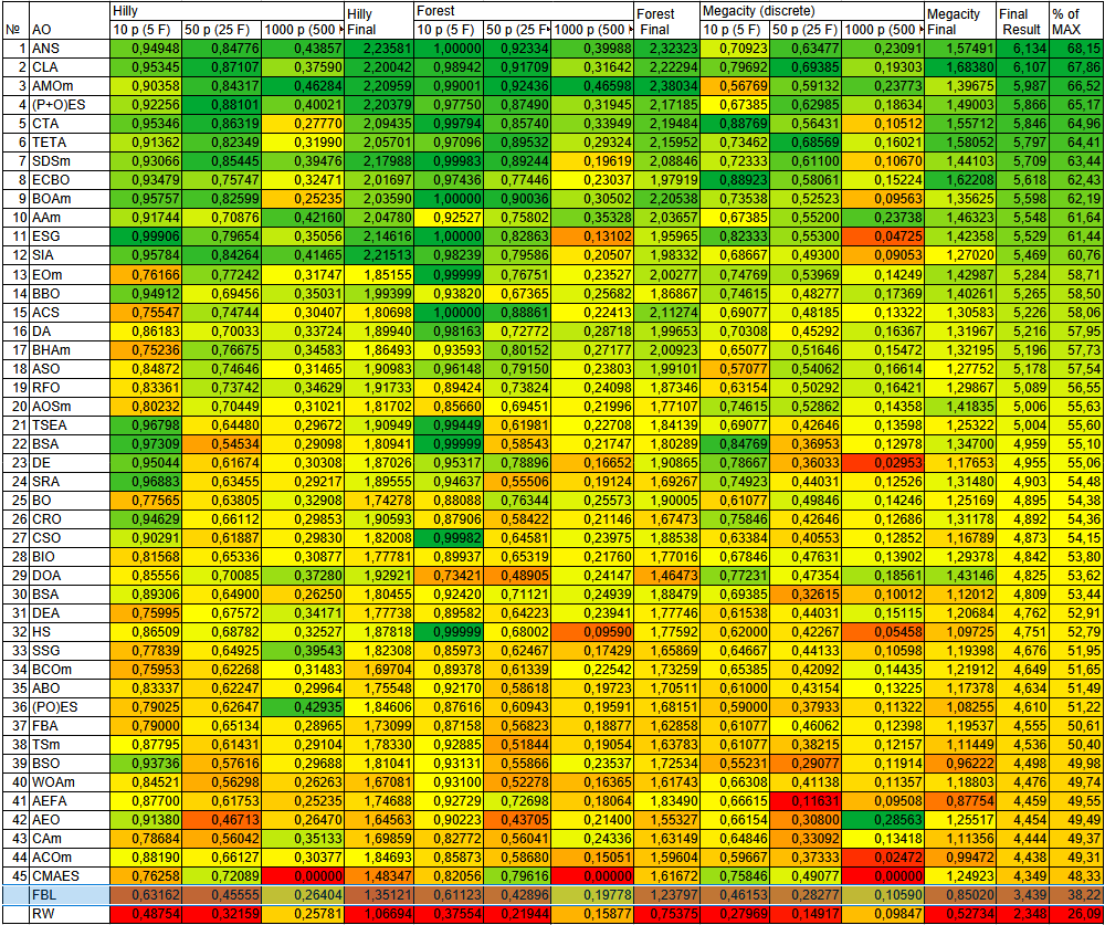
Figure 2. Color coding of algorithms for the corresponding tests
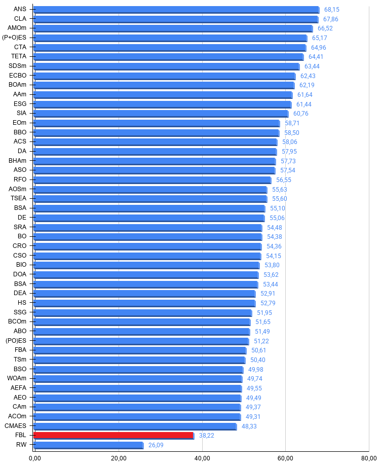
Figure 3. Histogram of the algorithm testing results (on a scale from 0 to 100, where higher is better, where 100 is the maximum possible theoretical result); the archive contains a script for calculating the ranking table
Pros and Cons of the FBL Algorithm
Pros:
- Good performance on problems with high dimensionality.
Cons:
- Weak convergence.
- Computational complexity.
An archive containing the latest versions of the algorithm source code is attached to the article. The author of this article does not claim absolute accuracy in the descriptions of the canonical algorithms; many of them have been modified to improve their search capabilities. The conclusions and judgments presented in the articles are based on the results of the experiments conducted.
Programs used in the article
| # | Name | Type | Description |
|---|---|---|---|
| 1 | #C_AO.mqh | Include file | Parent class of population-based optimization algorithms |
| 2 | #C_AO_enum.mqh | Include file | Enumeration of population-based optimization algorithms |
| 3 | TestFunctions.mqh | Include file | Test functions library |
| 4 | TestStandFunctions.mqh | Include file | Test bench function library |
| 5 | TestStand3D.mqh | Include file | 3D visualization panel for the test bench |
| 6 | Utilities.mqh | Include file | Utility function library |
| 7 | CalculationTestResults.mqh | Include file | Script for calculating results for a comparison table |
| 8 | Testing AOs.mq5 | Script | A unified test bench for all population-based optimization algorithms |
| 9 | Simple use of population optimization algorithms.mq5 | Script | A simple example of using population-based optimization algorithms without visualization |
| 10 | Test_FBL.mq5 | Script | Test bench for FBL |
Translated from Russian by MetaQuotes Ltd.
Original article: https://www.mql5.com/ru/articles/21821
Warning: All rights to these materials are reserved by MetaQuotes Ltd. Copying or reprinting of these materials in whole or in part is prohibited.
This article was written by a user of the site and reflects their personal views. MetaQuotes Ltd is not responsible for the accuracy of the information presented, nor for any consequences resulting from the use of the solutions, strategies or recommendations described.

 Monthly Profit and Loss Calendar Heatmap Renderer in MQL5
 Developing Smart Chart Objects in MQL5 (Part 2): Automating Trendline Discovery and Lifecycle Management
 Inside MetaEditor's AI Assistant: Writing, Repairing and Testing MQL5 with an Agent
 Meta-Labeling the Classics (Part 4): Filtering and Sizing MACD Trades

- Free trading apps
- Over 8,000 signals for copying
- Economic news for exploring financial markets
You agree to website policy and terms of use