Artificial Searching Swarm Algorithm (ASSA)

Table of Contents

1. Introduction
2. Algorithm Implementation
3. Test Results
4. Conclusions

Introduction

The global optimization problem arises in many applied fields — from engineering to automated trading systems — and, in real-world application scenarios, often involves multimodal, discontinuous, and mixed-type spaces where classical gradient methods are not applicable. Under these conditions, metaheuristics — including swarm algorithms — are in high demand. In this article, we examine the Artificial Searching Swarm Algorithm (ASSA) — an algorithm with an unusual tactical metaphor, in which agents exchange brief “signals” about the improvements they have found. Our testable hypothesis is whether such a short-lived signal can accelerate early convergence without compromising the swarm's ability to escape from local extrema under a fixed computational budget.

To answer this question, we implemented ASSA in MQL5 as a class compatible with the unified test bench, clearly formalized the three movement rules — synergy, search movement, and random movement — the mechanisms for normalization and handling discreteness, and conducted reproducible experiments on a standard set (Hilly, Forest, Megacity), supplemented with the benchmark functions Rosenbrock and Griewank. The evaluation criteria are solution quality within a fixed budget, stability across runs, and the behavior of the swarm dynamics.

The Artificial Searching Swarm Algorithm (ASSA) was published in 2012. This paper presents the results of testing ASSA on ten benchmark functions — ranging from the classic Rosenbrock, Griewank, and Rastrigin functions to constrained problems — and compares the results with those of a genetic algorithm, PSO, and AFSA. The authors show that, given a sufficient number of iterations, ASSA consistently outperforms its competitors in high-dimensional problems, while remaining simple to implement and insensitive to initial conditions.

Mathematically, the behavior of each agent is described by three mutually exclusive movement rules. The Synergistic Movement rule is triggered with probability "Pc" when an active call signal is present: the agent takes a step toward the calling agent's coordinates, with the step length proportional to the normalized distance to the target and to a random multiplier. The search rule is triggered when there is no signal: the agent generates a probe point by being drawn simultaneously toward its own personal best position and the swarm’s global best, and takes a step in the calculated direction. If, however, the probe coincides with the agent’s current position — meaning that there is no better personal or global reference point nearby — a stochastic rule is activated: a random step in an arbitrary direction, which supports exploratory activity and protects the algorithm from premature stagnation. When any of the three movements brings the agent to a point with a better function value, it immediately broadcasts its coordinates, and the signaling cycle resumes.

The global bulletin board mechanism, known in the biomimetic literature as the "Bulletin Board," serves as the algorithm's long-term memory. Unlike PSO, where each particle carries complete information about its trajectory, in ASSA each agent stores only its own personal best; the current global best for the entire swarm is updated centrally and is accessible to all agents simultaneously.

Algorithm Implementation

At each iteration of the ASSA algorithm, each agent performs exactly one move, selecting its type from among three possible rules depending on the current state of the system.

The swarm is controlled by a signaling mechanism. When any agent finds a position with a better fitness value than the one it had in the previous iteration, it broadcasts its coordinates. This position is stored in the "Xcall" variable and remains active for exactly one iteration. In the next iteration, each agent knows whether a signal was detected in the previous iteration and decides, with probability "Pc," whether to respond to it. If no agent improves during an iteration, the signal fades, and all agents switch to autonomous exploration mode.

At the same time, a global bulletin board (Bulletin Board) is maintained — a constantly updated record of the best position and the best fitness function value over the entire run of the algorithm. This is a global reference point available to every agent when choosing a direction of movement.

In addition to these two mechanisms, each agent maintains its own personal best — the best position and the best value it has personally found so far. Thus, three reference points are stored: the agent's current position, its personal best, and the global best solution of the entire swarm.

Three Movement Rules. All agent movements are implemented in a normalized search space. Normalization is necessary so that coordinates with different scales contribute equally to the calculation of distance and direction. The normalized Euclidean distance between two points "A" and "B" in an "n"-dimensional space is calculated as

NormDist(A, B) = sqrt( Σ ((A[c] - B[c]) / (ub[c] - lb[c]))² ),

where "ub" and "lb" are the upper and lower bounds of the search space for coordinate "c".

The step size in normalized space is specified by the "stepRatio" parameter, whose recommended values are in the range 0.15–0.30. In absolute units, for each coordinate this is:

stepRatio · (ub − lb).

Rule 1 — Synergistic Movement. It applies if a call signal was recorded in the previous iteration (callActive = true) and the random number r₀ ∈ [0, 1] was less than the probability parameter "Pc". The agent takes one step toward the caller’s position, "Xcall":

X_new[c] = X[c] + (Xcall[c] − X[c]) / NormDist(X, Xcall) · r₁ · stepRatio

Dividing by "NormDist" turns the direction vector into a unit vector in normalized space, so the actual step length along each coordinate is exactly r₁ · stepRatio · (ub − lb), regardless of the coordinate scale. The multiplier r₁ ∈ [0, 1] introduces randomness into the step length: the agent does not always take a full step.

The purpose of the rule is to quickly pull the swarm toward the region where an improvement has just been found. This is the primary mechanism for accelerating the algorithm’s convergence.

Rule 2 — Search Movement. It applies if there is no signal or if the agent did not respond to it. The agent constructs a probe point by being attracted simultaneously to its personal best "cB_i" and to the global best "cB":

probe[c] = X[c] + r₁ · (cB_i[c] − X[c]) + r₂ · (cB[c] − X[c]),

where r₁, r₂ ∈ [0, 1] are independent random numbers.

If the personal best coincides with the current position (or if both bests are already nearby), the probe barely moves from its place; this is a degenerate situation, and the algorithm proceeds to Rule 3.

Before calculating the distance, the probe is clamped to the bounds of the search space. This is fundamentally important: when r₁ + r₂ > 1, the "probe" point can go significantly beyond the feasible region, which will inflate "NormDist" to huge values and effectively reduce the agent’s actual step to zero. After clipping, the agent takes a step toward the probe:

X_new[c] = X[c] + (probe[c] − X[c]) / NormDist(X, probe) · r₃ · stepRatio.

The purpose of the rule is to use accumulated collective memory for directed search near known promising regions, while avoiding stagnation.

Rule 3 — Random Movement. This is applied if the probe point from Rule 2 almost coincides with the agent's current position (NormDist < 1e-10), indicating the absence of a useful gradient signal. The agent takes a random step for each coordinate independently:

X_new[c] = X[c] + rand(−1, 1) · stepRatio · (ub[c] − lb[c])

Purpose of the rule: to maintain exploratory activity and move the agent out of a stagnation point where neither the personal best nor the global best provides a direction for movement.

After any of the three moves, the new position is passed through the "SeInDiSp" function, which ensures correctness in discrete search spaces.

State Update. After the external evaluator has computed the fitness-function values for all new positions, the algorithm updates its internal state. For each individual, the system checks whether its result has improved compared to the previous iteration. The agent with the best newly obtained fitness value among those that improved becomes the new source of the call signal for the next iteration — its position is recorded in "Xcall." If none of the agents has improved, the call signal is deactivated (callActive = false).

Regardless of whether an improvement is found, each agent unconditionally accepts its new position as the current position: unlike some algorithms, where rejected moves are discarded, in ASSA the agent always moves to the position it has just stepped to. This ensures continuous exploration of the search space even when no progress is being made.

An agent's personal best is updated only when an improvement occurs. The global bulletin board is updated as soon as any agent improves on the result recorded on it.

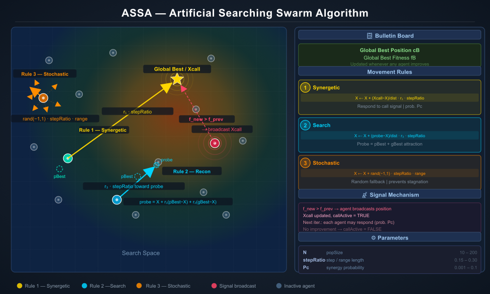
Figure 1. Illustration of the algorithm in operation

The illustration shows all the key elements of the algorithm in a single frame. The left side shows the search space: the background gradient mimics the fitness-function landscape, and the gold star with rings represents the global best / Xcall.

Three color-coded agents demonstrate each rule: the yellow arrow (Rule 1) flies toward "Xcall", the cyan arrow (Rule 2) moves to the "probe" point via the personal best and global best, and the orange arrows (Rule 3) fan out in random directions. The red agent with pulsing rings shows the moment of the signal. Gray inactive agents — the swarm background.

Right panel:

• Bulletin Board with "cB" and "fB" fields
• Three rule blocks with formulas
• Signal mechanism: four steps from improvement to flag clearing
• Table of parameters with recommended ranges.

Now let's write the pseudocode for the ASSA algorithm.

=== INITIALIZATION ===
FOR i = 0 TO N-1:
FOR c = 0 TO n-1:
X[i][c] ← a random number drawn from [lb[c], ub[c]]
callActive ← FALSE
revision ← FALSE

=== FIRST EVALUATION (revision = FALSE) ===
Moving:
FOR i = 0 TO N-1:
a[i].c ← SeInDiSp(X[i]) // snap to the grid
[the external evaluator computes a[i].f for all i]
Revision:
FOR i = 0 TO N-1:
a[i].fP ← a[i].f // baseline value for the improvement detector
a[i].fB ← a[i].f // personal best
a[i].cB ← a[i].c // personal best position
a[i].cP ← a[i].c // current position
IF a[i].f > fB:
fB ← a[i].f
cB ← a[i].c // global bulletin board

Xcall ← cB // initial signal from the best agent
callActive ← TRUE
revision ← TRUE

=== MAIN LOOP ===
WHILE the budget is not exhausted:
// --- MOVING ---
FOR i = 0 TO N-1:
moved ← FALSE

// RULE 1 — Synergistic Movement
IF callActive AND rand(0,1) < Pc:
dist ← NormDist(a[i].cP, Xcall)
IF dist > 1e-10:
r₁ ← rand(0, 1)
FOR c = 0 TO n-1:
xNew ← a[i].cP[c] + (Xcall[c] − a[i].cP[c]) / dist · r₁ · stepRatio
a[i].c[c] ← SeInDiSp(Clamp(xNew, lb[c], ub[c]))
moved ← TRUE

IF NOT moved:
// RULE 2 — Search Movement
r₁ ← rand(0, 1)
r₂ ← rand(0, 1)
FOR c = 0 TO n-1:
probe[c] ← Clamp(a[i].cP[c] + r₁·(a[i].cB[c] − a[i].cP[c])
+ r₂·(cB[c] − a[i].cP[c]),
lb[c], ub[c])
dist ← NormDist(a[i].cP, probe)

IF dist > 1e-10:
r₃ ← rand(0, 1)
FOR c = 0 TO n-1:
xNew ← a[i].cP[c] + (probe[c] − a[i].cP[c]) / dist · r₃ · stepRatio
a[i].c[c] ← SeInDiSp(Clamp(xNew, lb[c], ub[c]))
ELSE:
// RULE 3 — Random Movement
FOR c = 0 TO n-1:
xNew ← a[i].cP[c] + rand(−1, 1) · stepRatio · (ub[c] − lb[c])
a[i].c[c] ← SeInDiSp(Clamp(xNew, lb[c], ub[c]))
[the external evaluator computes a[i].f for all i]

// --- REVISION ---
newCall ← FALSE
bestImpr ← −∞

FOR i = 0 TO N-1:
// improvement detector → candidate for a new signal
IF a[i].f > a[i].fP AND a[i].f > bestImpr:
bestImpr ← a[i].f
newCall ← TRUE
Xcall ← a[i].c

// update personal best
IF a[i].f > a[i].fB:
a[i].fB ← a[i].f
a[i].cB ← a[i].c

// unconditionally accept the new position
a[i].fP ← a[i].f
a[i].cP ← a[i].c

// update the global bulletin board
IF a[i].f > fB:
fB ← a[i].f
cB ← a[i].c

callActive ← newCall

=== RESULT ===
RETURN cB, fB // position and value of the global optimum

Let's move on to writing the code for the algorithm. The "C_AO_ASSA" class inherits from the base class "C_AO" and implements all three behavioral rules of the Artificial Searching Swarm Algorithm. The class's public interface is identical to that of the other algorithms in the "C_AO" series: the "Init", "Moving", and "Revision" methods make it compatible with the unified test bench without requiring any changes to the external code.

The algorithm uses the following fields from the base class: a[] — an array of agents; a[i].c[] — the position for evaluating the fitness function; a[i].f — the fitness function value, populated by an external evaluator; a[i].cP[] — the agent’s current position, saved between iterations; a[i].cB[] and a[i].fB — the position and value of the personal best; a[i].fP — the fitness function value at the previous position, used to detect improvements; cB[] and fB — the global bulletin board (the position and value of the best solution found over the entire run); revision — a flag indicating completion of the initialization phase.

The class's own fields, which have no counterparts in the base class, consist of only four elements: "stepRatio" stores the search step as a fraction of the range length along each axis, "Pc" specifies the probability of Synergistic Movement, and "callActive" is a Boolean flag indicating the presence of an active call signal that remains active for exactly one iteration. Xcall[] — an array of coordinates that records the position of the agent that most recently broadcast an improvement. The probe[] working array is allocated once during initialization and reused in each iteration to compute the probe point for Rule 2.

The SetParams method transfers values from the universal params[] array to the typed fields of the class. It is called once from the test script after the user has specified the required values via the input parameters.

//————————————————————————————————————————————————————————————————————
class C_AO_ASSA : public C_AO
{
  public: //----------------------------------------------------------
  ~C_AO_ASSA () { }
  C_AO_ASSA ()
  {
    ao_name = "ASSA";
    ao_desc = "Artificial Searching Swarm Algorithm";
    ao_link = "https://www.mql5.com/en/articles/21671";

    popSize   = 20;
    stepRatio = 0.25;
    Pc        = 0.01;

    ArrayResize (params, 3);
    params [0].name = "popSize";   params [0].val = popSize;
    params [1].name = "stepRatio"; params [1].val = stepRatio;   // AS_step = stepRatio * (ub - lb), recommended range 0.15–0.30
    params [2].name = "Pc";        params [2].val = Pc;          // synergistic probability, recommended range: 0.001–0.1
  }

  void SetParams ()
  {
    popSize   = (int)params [0].val;
    stepRatio =      params [1].val;
    Pc        =      params [2].val;
  }

  bool Init (const double &rangeMinP  [],
             const double &rangeMaxP  [],
             const double &rangeStepP [],
             const int     epochsP = 0);

  void Moving   ();
  void Revision ();

  //------------------------------------------------------------------
  double stepRatio;   // step as a fraction of the search range length
  double Pc;          // probability that an agent responds to a call (Rule 1)

  private: //---------------------------------------------------------
  double Xcall [];    // position of the agent that last sent a call
  bool   callActive;  // is there an active call signal?
  double probe [];    // reusable workspace for the Rule-2 candidate point (avoids per-call allocation)

  // Returns the Euclidean distance in coordinate-normalized space [0,1]^n.
  // Normalizing by (ub-lb) per coordinate makes the steps scale-independent.
  double NormDist (double &A [], double &B []);
};
//————————————————————————————————————————————————————————————————————

The initialization method prepares the algorithm for a new run. First, the base class's "StandardInit" method is called; it sets the "revision" flag to "false," resets the global best "fB," allocates and initializes the agent array a[], and copies the specified search ranges into internal arrays. After returning from "StandardInit," memory is allocated for the class's own arrays: Xcall[] of size "coords" to store the signal position, and probe[] of the same size for the working computation of the probe. The "callActive" flag is set to "false" — there is no signal yet.

Next, each agent is placed in a random initial position: for each coordinate, u.RNDfromCI is called, and the result is stored in a[i].cP[c]. It is cP[], not c[], that represents the agent's current position between iterations. The c[] field is not populated at this stage — it will be set the first time "Moving" is called.

//————————————————————————————————————————————————————————————————————
bool C_AO_ASSA::Init (const double &rangeMinP  [],
                      const double &rangeMaxP  [],
                      const double &rangeStepP [],
                      const int     epochsP = 0)
{
  if (!StandardInit (rangeMinP, rangeMaxP, rangeStepP)) return false;

  //------------------------------------------------------------------
  ArrayResize (Xcall, coords);
  ArrayResize (probe, coords);

  callActive = false;

  // Place agents at random positions; cP[] is the "live" position between iterations.
  for (int i = 0; i < popSize; i++)
    for (int c = 0; c < coords; c++)
      a [i].cP [c] = u.RNDfromCI (rangeMin [c], rangeMax [c]);

  return true;
}
//————————————————————————————————————————————————————————————————————

The auxiliary method calculates the Euclidean distance between two points "A" and "B" in the normalized space [0, 1]^n. Normalization is performed coordinate by coordinate.

The return value serves two purposes. First, as the divisor for normalizing the direction vector — it is precisely the division by "NormDist" that transforms the vector (TO − X) into a unit vector in the normalized space, and then the product r · stepRatio defines the step length as a fraction of the range, regardless of the absolute scale. Second, as a threshold check — if the distance is less than 1e-10, Rule 2 considers the probe to coincide with the current position and transfers control to Rule 3.

//————————————————————————————————————————————————————————————————————
double C_AO_ASSA::NormDist (double &A [], double &B [])
{
  double s = 0.0;
  for (int c = 0; c < coords; c++)
  {
    double rng = rangeMax [c] - rangeMin [c];
    if (rng < 1e-10) continue;
    double d = (A [c] - B [c]) / rng;
    s += d * d;
  }
  return MathSqrt (s);
}
//————————————————————————————————————————————————————————————————————

The method implements the movement phase for all agents and is divided into two fundamentally different blocks. In the very first "Moving" call, the "revision" flag is still false — initialization is not complete. In this case, the method simply maps the initial positions from a[i].cP[] to a[i].c[] using u.SeInDiSp(), snapping each coordinate to the nearest valid node on the discrete grid. These values will be passed to an external evaluator, which will compute the initial values of the fitness function. No movement takes place yet.

Normal iterations (when revision = true). For each agent, the method checks three rules sequentially, moving on to the next one only if the previous one did not apply. The "moved" flag tracks whether a move was made according to Rule 1.

Rule 1 — Synergistic Movement. The method checks both whether the "callActive" signal is active and whether the random number u.RNDfromCI(0,1) is less than Pc. If both conditions are met, the normalized distance from the current position a[i].cP to the "Xcall" signal position is calculated. If the distance is nonzero, a random number "r1" is drawn, and the following step is performed: xNew = cP[c] + (Xcall[c] − cP[c]) / dist * r1 * stepRatio. The result is clamped to the bounds using the Clamp() helper method and SeInDiSp(). The "moved" flag is set.

Rule 2 — Search Movement. Executed if "moved" is false. "r1" and "r2" are drawn independently, after which the probe is calculated for each coordinate: probe[c] = cP[c] + r1*(cB_i[c] − cP[c]) + r2*(cB[c] − cP[c]). The probe is immediately clamped to the bounds—this is a crucial step: when r1 + r2 > 1, the raw probe value leaves the feasible region, and without “NormDist” it inflates to values at which the agent’s actual step degenerates to zero. After that, the normalized distance to the probe is calculated; if the distance is nonzero, "r3" is drawn, and a step is taken in the direction of the probe.

Rule 3 — Random Movement. This applies if the "NormDist" to the probe is less than the threshold of 1e-10, meaning the probe practically coincides with the agent's current position. A random offset is applied independently to each coordinate: xNew = cP[c] + u.RNDfromCI(−1, 1) * stepRatio * (rangeMax[c] − rangeMin[c]).

In all three cases, the final "xNew" is passed through SeInDiSp() before being written to a[i].c[c].

//————————————————————————————————————————————————————————————————————
void C_AO_ASSA::Moving ()
{
  //--- Pass 0 (before the first Revision): expose initial random positions
  // `revision` is the base-class flag; it is false until `Revision()` sets it to true.
  if (!revision)
  {
    for (int i = 0; i < popSize; i++)
    {
      for (int c = 0; c < coords; c++)
      {
        a [i].c [c] = u.SeInDiSp (a [i].cP [c], rangeMin  [c], rangeMax  [c], rangeStep [c]);
      }
    }
    return;
  }

  //--- Normal iterations --------------------------------------------
  for (int i = 0; i < popSize; i++)
  {
    bool moved = false;

    //================================================================
    // RULE 1 — Synergistic Movement
    //   If an active call exists AND rand < Pc, move one step toward Xcall.
    //
    //   Formula (normalized-space step toward Xcall):
    //     X_new[c] = X[c] + (Xcall[c] - X[c]) / NormDist(X, Xcall) * r1 * stepRatio
    //
    //   Division by NormDist converts the real-space direction vector into
    //   a unit vector in normalized space, so the step length equals
    //   r1 * stepRatio * (ub[c] - lb[c]), regardless of the coordinate scale.
    //================================================================
    if (callActive && u.RNDfromCI (0.0, 1.0) < Pc)
    {
      double dist = NormDist (a [i].cP, Xcall);
      if (dist > 1e-10)
      {
        double r1 = u.RNDfromCI (0.0, 1.0);
        for (int c = 0; c < coords; c++)
        {
          double xNew = a [i].cP [c]
                      + (Xcall [c] - a [i].cP [c]) / dist * r1 * stepRatio;
          a [i].c [c] = u.SeInDiSp (xNew, rangeMin [c], rangeMax [c], rangeStep [c]);
        }
        moved = true;
      }
    }

    if (!moved)
    {
      //==============================================================
      // RULE 2 — Search Move
      //   Build a candidate probe attracted toward the personal best (cB / Xs)
      //   and toward the global best (cB_global / Xg), then step toward it.
      //
      //   Probe formula:
      //     probe[c] = X[c] + r1*(Xs[c] - X[c]) + r2*(Xg[c] - X[c])
      //
      //   The probe is clamped to [lb, ub] before the direction is computed:
      //   When r1 + r2 &gt; 1, the raw probe flies outside the domain,
      //   causing NormDist to become very large and the actual step size to shrink to ~0.
      //
      //   Step formula (direction in normalized space toward the probe):
      //     X_new[c] = X[c] + (probe[c] - X[c]) / NormDist(X, probe) * r3 * stepRatio
      //
      //   Falls through to Rule 3 when probe == X (NormDist &lt; threshold).
      //==============================================================
      double r1 = u.RNDfromCI (0.0, 1.0);
      double r2 = u.RNDfromCI (0.0, 1.0);

      for (int c = 0; c < coords; c++)
      {
        probe [c] = a [i].cP [c] + r1 * (a [i].cB [c] - a [i].cP [c]) + r2 * (cB [c] - a [i].cP [c]);
      }

      double dist = NormDist (a [i].cP, probe);

      if (dist > 1e-10)
      {
        double r3 = u.RNDfromCI (0.0, 1.0);
        for (int c = 0; c < coords; c++)
        {
          double xNew = a [i].cP [c] + (probe [c] - a [i].cP [c]) / dist * r3 * stepRatio;
          a [i].c [c] = u.SeInDiSp (xNew, rangeMin [c], rangeMax [c], rangeStep [c]);
        }
      }
      else
      {
        //============================================================
        // RULE 3 — Stochastic move (fallback when probe == X)
        //   Random displacement in [-stepRatio, +stepRatio] * (ub - lb) per coordinate.
        //
        //   Formula:
        //     X_new[c] = X[c] + rand(-1, 1) * stepRatio * (ub[c] - lb[c])
        //============================================================
        for (int c = 0; c < coords; c++)
        {
          double xNew = a [i].cP [c] + u.RNDfromCI (-1.0, 1.0) * stepRatio * (rangeMax [c] - rangeMin [c]);
          a [i].c [c] = u.SeInDiSp (xNew, rangeMin [c], rangeMax [c], rangeStep [c]);
        }
      }
    }
  }
}
//————————————————————————————————————————————————————————————————————

The Revision method implements the phase of updating the algorithm's internal state after the external evaluator has filled in the values of a[i].f. Like "Moving", the method is divided into two blocks.

Zeroth-iteration pass (when revision = false). After the first evaluation of the fitness function, the method initializes all historical records. For each agent: the current value of a[i].f is stored in a[i].fP as a baseline for future improvement detection; the same value is stored in a[i].fB as the initial personal best; the position a[i].c is copied to a[i].cB and a[i].cP. At the same time, the global best is tracked: the best agent updates the "fB" and "cB" fields of the base class. Upon completion of the loop, the global best position is copied to "Xcall," and the "callActive" flag is set to "true" — so that agents can use the Synergistic Movement rule starting from the very first working iteration. The "revision" flag is set to "true," indicating that initialization is complete.

Normal iterations (when revision = true). Before the loop over agents, the variables used to detect a new signal are reset: newCall = false and bestImpr = −DBL_MAX. Then, four independent checks are performed for each agent.

First check: if a[i].f &gt; a[i].fP (the agent has improved compared to the previous iteration) and its new value is better than any other improvement in the current iteration, this agent becomes a new source of the call signal — its position is recorded in "Xcall," and the "newCall" flag is set.

Second check: if a[i].f > a[i].fB, the agent's personal best is updated — the agent's "fB" and "cB" are assigned new values.

Step 3: unconditional acceptance of the new position. a[i].fP is set to a[i].f, and a[i].cP is set to a[i].c. This is a deliberate architectural choice: in ASSA, the agent always moves to the location where it took its last step, regardless of whether that movement was an improvement. This unconditional diffusion supports continuous exploration of the search space.

Fourth check: if a[i].f > fB, the global bulletin board is updated. At the end of the loop, the "callActive" flag is set to "newCall". If no agent has improved, the call signal goes out, and on the next iteration all agents will switch to search mode or random movement.

//————————————————————————————————————————————————————————————————————
void C_AO_ASSA::Revision ()
{
  //--- Pass 0: first evaluation -> initialize all history records ---
  if (!revision)
  {
    for (int i = 0; i < popSize; i++)
    {
      a [i].fP = a [i].f;                           // baseline for detecting improvements
      a [i].fB = a [i].f;                           // personal best fitness
      ArrayCopy (a [i].cB, a [i].c, 0, 0, coords); // personal best position
      ArrayCopy (a [i].cP, a [i].c, 0, 0, coords); // live position (grid-snapped)

      if (a [i].f > fB)
      {
        fB = a [i].f;
        ArrayCopy (cB, a [i].c, 0, 0, coords);
      }
    }

    // Seed the call signal with the global best so Rule 1 is immediately useful.
    ArrayCopy (Xcall, cB, 0, 0, coords);
    callActive = true;

    revision = true; // base-class flag: the initialization phase is complete
    return;
  }

  //--- Normal revision: update records, detect improvements, manage the call signal
  //   The best-improving agent (highest new fitness) broadcasts its position
  //   as the call signal for the next iteration.
  bool   newCall  = false;
  double bestImpr = -DBL_MAX;

  for (int i = 0; i < popSize; i++)
  {
    // Detect improvement over the previous position -> this agent sends a call signal.
    if (a [i].f > a [i].fP && a [i].f > bestImpr)
    {
      bestImpr = a [i].f;
      newCall  = true;
      ArrayCopy (Xcall, a [i].c, 0, 0, coords);
    }

    // Update personal best (cB / Xs).
    if (a [i].f > a [i].fB)
    {
      a [i].fB = a [i].f;
      ArrayCopy (a [i].cB, a [i].c, 0, 0, coords);
    }

    // Accept the move unconditionally: the current position becomes the new baseline.
    a [i].fP = a [i].f;
    ArrayCopy (a [i].cP, a [i].c, 0, 0, coords);

    // Update global best — Bulletin Board (base fields cB / fB).
    if (a [i].f > fB)
    {
      fB = a [i].f;
      ArrayCopy (cB, a [i].c, 0, 0, coords);
    }
  }

  callActive = newCall;
}
//————————————————————————————————————————————————————————————————————

Test Results

ASSA's final score of 33.42% across the test series does not allow it to be included in the ranking of the top 45 optimization methods.

ASSA|Artificial Searching Swarm Algorithm|50.0|0.3|0.1|
=============================
5 Hilly's; Func runs: 10000; result: 0.6255894509557836
25 Hilly's; Func runs: 10000; result: 0.4138604978642843
500 Hilly's; Func runs: 10000; result: 0.25380653012476456
=============================
5 Forest's; Func runs: 10000; result: 0.5448792178119948
25 Forest's; Func runs: 10000; result: 0.2980777003474912
500 Forest's; Func runs: 10000; result: 0.185642399646027
=============================
5 Megacity's; Func runs: 10000; result: 0.41076923076923083
25 Megacity's; Func runs: 10000; result: 0.1787692307692308
500 Megacity's; Func runs: 10000; result: 0.09629230769230851
=============================
Total score: 3.00769 (33.42%)

Let's expand our set of test functions with two more widely accepted benchmark problems so that researchers can test algorithms on other types of landscapes as well. In particular, the Rosenbrock function is used to evaluate the accuracy of convergence, while the Griewank function — like the Rastrigin function — is used to analyze the rate and stability of convergence. While we are at it, let's see how the ASSA algorithm performs on these new test functions.

ASSA on the Griewank test function

The Griewank function was proposed by Andreas Griewank in 1980 in a paper on generalized descent methods for global optimization, and has since become a standard part of the benchmark suite for comparative testing of metaheuristics. In the two-dimensional case, it is written as follows: f(x, y) = (x² + y²) / 4000 − cos(x) · cos(y/√2) + 1

The structure of the function is a superposition of two fundamentally different components. The first is a quadratic paraboloid with a very gentle slope (the divisor 4,000 intentionally makes it almost flat), forming a general gradient background that directs the search toward the center. The second is the product of two cosines, creating a dense, periodic ripple across the entire surface. It is precisely the interaction of these two components that determines the complexity of the function: the cosine term generates a vast number of local optima, while the quadratic background makes them unequal — the farther from the center, the worse the local maximum. There is exactly one global optimum, located at the point (0, 0), where f(0, 0) = 0.

The asymmetry of the cells in the cosine grid deserves special attention. Along the x-axis, the period is 2π ≈ 6.28, whereas along the y-axis, the argument of the cosine is divided by √2, which extends the period to 2π√2 ≈ 8.89. As a result, in the 2D visualization, the characteristic "islands" of optima are not square but rectangular, elongated vertically — this is clearly visible in the function plot.

For the test bench, the search domain x, y ∈ [−20, 20] has been selected. The choice of this range is not arbitrary and warrants a separate explanation. In the literature, the standard search range for the Griewank function is defined as [−600, 600]. However, with this range, the cosine period is less than one percent of the screen width, and the characteristic grid of optima visually blends into a uniform background indistinguishable from a pure paraboloid.

With a range of [−20, 20], the field of view encompasses about six and a half periods along the "x" axis and about five along the "y" axis, while the amplitude of the cosine term exceeds the contribution of the quadratic term by a factor of five — the ripples become visually dominant, and the structure of the function is clearly discernible. From the perspective of algorithmic complexity, reducing the range decreases the total number of local optima, but does not change the fundamental nature of the problem: the algorithm is still forced to operate in a multimodal landscape, where every step risks falling into a neighboring local basin. In the multidimensional case (500 runs, i.e., 1,000 variables), the complexity of the problem increases manifold.

Since the test bench is designed for maximization, the Griewank function is included in it in its inverted form: instead of f(x, y), −f(x, y) is evaluated, which transforms the global minimum into a global maximum. Scaling to the range [0, 1] is performed relative to the maximum value of the original function, ≈ 2.141, which is reached near the point (−15.716, −17.798). The implementation of the Griewank function is shown below.

//——————————————————————————————————————————————————————————————————————————————
class C_Griewank : public C_Function
{
  public: //===================================================================
  C_Griewank ()
  {
    fuName = "Griewank";

    //function bounds
    xMinRange = -20.0; xMaxRange = 20.0;
    yMinRange = -20.0; yMaxRange = 20.0;

    //coordinates of the maximum (framework: minimum of the original function)
    globalMaxFunValue = 1.0;
    xGlobalMax        = 0.0;
    yGlobalMax        = 0.0;

    //coordinates of the minimum (framework: maximum of the original function)
    globalMinFunValue = 0.0;
    xGlobalMin        = -15.715716;
    yGlobalMin        = -17.797798;
  }

  double Core (double x, double y)
  {
    double f = (x * x + y * y) / 4000.0
             - MathCos (x) * MathCos (y / MathSqrt (2.0))
             + 1.0;

    // Invert: the minimum of the original f → the maximum on the [0, 1] scale
    return Scale (-f, -2.140734, 0.0, 0.0, 1.0);
  }
};
//——————————————————————————————————————————————————————————————————————————————

Another function: implementation and visualization.

ASSA on the Rosenbrock test function

The Rosenbrock function was published in 1960 and remains to this day one of the most frequently cited tests for optimization algorithms — not because of an abundance of local optima, but for the exact opposite reason. In the two-dimensional case, it is given by the formula: f(x, y) = 100·(y − x²)² + (1 − x)²

The function has a single global minimum, f(1, 1) = 0, and no local minima — it would seem to be the simplest problem for any optimizer. However, it is precisely the topology of its landscape that makes it a classic challenge. The minimum lies at the bottom of a narrow, highly curved parabolic valley oriented along the curve y = x². The transverse gradient in this valley is enormous — even the slightest deviation from the valley floor causes a sharp increase in the function's value. The longitudinal gradient along the valley floor, however, is extremely gentle: the function decreases toward its minimum slowly and almost imperceptibly to algorithms that focus on the amount of improvement per step, making it very well suited for determining the convergence accuracy of algorithms.

The characteristic shape of the landscape is clearly visible in the 2D visualization: the red region of high values (i.e., low values of the original function in the inverted representation) is elongated along a curved band that follows the parabola y = x², while the lower-left corner transitions to blue — precisely there, at the point (−2.048, −2.048), the original function reaches its maximum ≈ 3905.926, which corresponds to zero on the framework scale.

The difficulty Rosenbrock poses for swarm algorithms is of a specific kind. Most metaheuristics work effectively when the search space contains clear landmarks — distinct peaks that attract agents. Here, however, an agent that has reached the bottom of the valley finds itself in a situation where there is almost no gradient signal along the path toward the optimum. An algorithm capable of reliably finding the point (1, 1) demonstrates the ability to navigate a barely perceptible slope without sliding off the slippery walls of the valley. In the multidimensional case, the problem becomes exponentially more complex: a valley in “n” dimensions becomes an n-dimensional parabolic tube, and the probability of accidentally escaping from it increases with each additional dimension.

The search region for the test bench is defined as x, y ∈ [−2.048, 2.048] — a standard range used in most comparative studies. The function is also included in the test bench in its inverted form: −f(x, y) is evaluated, and the global minimum becomes a global maximum with a value of 1.0 on the normalized scale. The implementation is shown below.

//——————————————————————————————————————————————————————————————————————————————
class C_Rosenbrock : public C_Function
{
  public: //===================================================================
  C_Rosenbrock ()
  {
    fuName = "Rosenbrock";

    //function bounds
    xMinRange = -2.048; xMaxRange = 2.048;
    yMinRange = -2.048; yMaxRange = 2.048;

    //coordinates of the maximum (framework: minimum of the original function)
    globalMaxFunValue = 1.0;
    xGlobalMax        = 1.0;
    yGlobalMax        = 1.0;

    //coordinates of the minimum (framework: maximum of the original function)
    globalMinFunValue = 0.0;
    xGlobalMin        = -2.048;
    yGlobalMin        = -2.048;
  }

  double Core (double x, double y)
  {
    double f = 100.0 * MathPow (y - x * x, 2) + MathPow (1.0 - x, 2);

    // Invert: the minimum of the original f → the maximum on the [0, 1] scale
    return Scale (-f, -3905.926227, 0.0, 0.0, 1.0);
  }
};
//——————————————————————————————————————————————————————————————————————————————

Visualization of ASSA's performance on test functions for determining the ranking.

ASSA on the Hilly test function

ASSA on the Forest test function

ASSA on the Megacity test function

After a series of tests, the ASSA algorithm is included in our ranking table of the best optimization methods for informational purposes only.

No.	AO	Description	Hilly			Hilly Final	Forest			Forest Final	Megacity (discrete)			Megacity Final	Final Result	% of MAX
			10 p (5 F)	50 p (25 F)	1000 p (500 F)		10 p (5 F)	50 p (25 F)	1000 p (500 F)		10 p (5 F)	50 p (25 F)	1000 p (500 F)
1	ANS	across neighbourhood search	0.94948	0.84776	0.43857	2.23581	1.00000	0.92334	0.39988	2.32323	0.70923	0.63477	0.23091	1.57491	6.134	68.15
2	CLA	code lock algorithm (joo)	0.95345	0.87107	0.37590	2.20042	0.98942	0.91709	0.31642	2.22294	0.79692	0.69385	0.19303	1.68380	6.107	67.86
3	AMOm	animal migration optimization M	0.90358	0.84317	0.46284	2.20959	0.99001	0.92436	0.46598	2.38034	0.56769	0.59132	0.23773	1.39675	5.987	66.52
4	(P+O)ES	(P+O) evolution strategies	0.92256	0.88101	0.40021	2.20379	0.97750	0.87490	0.31945	2.17185	0.67385	0.62985	0.18634	1.49003	5.866	65.17
5	CTA	comet tail algorithm (joo)	0.95346	0.86319	0.27770	2.09435	0.99794	0.85740	0.33949	2.19484	0.88769	0.56431	0.10512	1.55712	5.846	64.96
6	TETA	time-evolution travel algorithm (joo)	0.91362	0.82349	0.31990	2.05701	0.97096	0.89532	0.29324	2.15952	0.73462	0.68569	0.16021	1.58052	5.797	64.41
7	SDSm	stochastic diffusion search M	0.93066	0.85445	0.39476	2.17988	0.99983	0.89244	0.19619	2.08846	0.72333	0.61100	0.10670	1.44103	5.709	63.44
8	ECBO	enhanced_colliding_bodies_optimization	0.93479	0.75747	0.32471	2.01697	0.97436	0.77446	0.23037	1.97919	0.88923	0.58061	0.15224	1.62208	5.618	62.43
9	BOAm	billiards optimization algorithm M	0.95757	0.82599	0.25235	2.03590	1.00000	0.90036	0.30502	2.20538	0.73538	0.52523	0.09563	1.35625	5.598	62.19
10	AAm	archery algorithm M	0.91744	0.70876	0.42160	2.04780	0.92527	0.75802	0.35328	2.03657	0.67385	0.55200	0.23738	1.46323	5.548	61.64
11	ESG	evolution of social groups (joo)	0.99906	0.79654	0.35056	2.14616	1.00000	0.82863	0.13102	1.95965	0.82333	0.55300	0.04725	1.42358	5.529	61.44
12	SIA	simulated isotropic annealing (joo)	0.95784	0.84264	0.41465	2.21513	0.98239	0.79586	0.20507	1.98332	0.68667	0.49300	0.09053	1.27020	5.469	60.76
13	EOm	extremal_optimization_M	0.76166	0.77242	0.31747	1.85155	0.99999	0.76751	0.23527	2.00277	0.74769	0.53969	0.14249	1.42987	5.284	58.71
14	BBO	biogeography-based optimization	0.94912	0.69456	0.35031	1.99399	0.93820	0.67365	0.25682	1.86867	0.74615	0.48277	0.17369	1.40261	5.265	58.50
15	ACS	artificial cooperative search	0.75547	0.74744	0.30407	1.80698	1.00000	0.88861	0.22413	2.11274	0.69077	0.48185	0.13322	1.30583	5.226	58.06
16	DA	dialectical algorithm	0.86183	0.70033	0.33724	1.89940	0.98163	0.72772	0.28718	1.99653	0.70308	0.45292	0.16367	1.31967	5.216	57.95
17	BHAm	black hole algorithm M	0.75236	0.76675	0.34583	1.86493	0.93593	0.80152	0.27177	2.00923	0.65077	0.51646	0.15472	1.32195	5.196	57.73
18	ASO	anarchy society optimization	0.84872	0.74646	0.31465	1.90983	0.96148	0.79150	0.23803	1.99101	0.57077	0.54062	0.16614	1.27752	5.178	57.54
19	RFO	royal flush optimization (JOO)	0.83361	0.73742	0.34629	1.91733	0.89424	0.73824	0.24098	1.87346	0.63154	0.50292	0.16421	1.29867	5.089	56.55
20	AOSm	atomic orbital search M	0.80232	0.70449	0.31021	1.81702	0.85660	0.69451	0.21996	1.77107	0.74615	0.52862	0.14358	1.41835	5.006	55.63
21	TSEA	turtle shell evolution algorithm (JOO)	0.96798	0.64480	0.29672	1.90949	0.99449	0.61981	0.22708	1.84139	0.69077	0.42646	0.13598	1.25322	5.004	55.60
22	BSA	backtracking_search_algorithm	0.97309	0.54534	0.29098	1.80941	0.99999	0.58543	0.21747	1.80289	0.84769	0.36953	0.12978	1.34700	4.959	55.10
23	DE	differential evolution	0.95044	0.61674	0.30308	1.87026	0.95317	0.78896	0.16652	1.90865	0.78667	0.36033	0.02953	1.17653	4.955	55.06
24	SRA	successful restaurateur algorithm (JOO)	0.96883	0.63455	0.29217	1.89555	0.94637	0.55506	0.19124	1.69267	0.74923	0.44031	0.12526	1.31480	4.903	54.48
25	BO	bonobo_optimizer	0.77565	0.63805	0.32908	1.74278	0.88088	0.76344	0.25573	1.90005	0.61077	0.49846	0.14246	1.25169	4.895	54.38
26	CRO	chemical reaction optimization	0.94629	0.66112	0.29853	1.90593	0.87906	0.58422	0.21146	1.67473	0.75846	0.42646	0.12686	1.31178	4.892	54.36
27	BIO	blood inheritance optimization (JOO)	0.81568	0.65336	0.30877	1.77781	0.89937	0.65319	0.21760	1.77016	0.67846	0.47631	0.13902	1.29378	4.842	53.80
28	DOA	dream_optimization_algorithm	0.85556	0.70085	0.37280	1.92921	0.73421	0.48905	0.24147	1.46473	0.77231	0.47354	0.18561	1.43146	4.825	53.62
29	BSA	bird swarm algorithm	0.89306	0.64900	0.26250	1.80455	0.92420	0.71121	0.24939	1.88479	0.69385	0.32615	0.10012	1.12012	4.809	53.44
30	DEA	dolphin_echolocation_algorithm	0.75995	0.67572	0.34171	1.77738	0.89582	0.64223	0.23941	1.77746	0.61538	0.44031	0.15115	1.20684	4.762	52.91
31	HS	harmony search	0.86509	0.68782	0.32527	1.87818	0.99999	0.68002	0.09590	1.77592	0.62000	0.42267	0.05458	1.09725	4.751	52.79
32	SSG	saplings sowing and growing	0.77839	0.64925	0.39543	1.82308	0.85973	0.62467	0.17429	1.65869	0.64667	0.44133	0.10598	1.19398	4.676	51.95
33	BCOm	bacterial chemotaxis optimization M	0.75953	0.62268	0.31483	1.69704	0.89378	0.61339	0.22542	1.73259	0.65385	0.42092	0.14435	1.21912	4.649	51.65
34	ABO	african buffalo optimization	0.83337	0.62247	0.29964	1.75548	0.92170	0.58618	0.19723	1.70511	0.61000	0.43154	0.13225	1.17378	4.634	51.49
35	(PO)ES	(PO) evolution strategies	0.79025	0.62647	0.42935	1.84606	0.87616	0.60943	0.19591	1.68151	0.59000	0.37933	0.11322	1.08255	4.610	51.22
36	FBA	fractal-based algorithm	0.79000	0.65134	0.28965	1.73099	0.87158	0.56823	0.18877	1.62858	0.61077	0.46062	0.12398	1.19537	4.555	50.61
37	TSm	tabu search M	0.87795	0.61431	0.29104	1.78330	0.92885	0.51844	0.19054	1.63783	0.61077	0.38215	0.12157	1.11449	4.536	50.40
38	BSO	brain storm optimization	0.93736	0.57616	0.29688	1.81041	0.93131	0.55866	0.23537	1.72534	0.55231	0.29077	0.11914	0.96222	4.498	49.98
39	WOAm	whale optimization algorithm M	0.84521	0.56298	0.26263	1.67081	0.93100	0.52278	0.16365	1.61743	0.66308	0.41138	0.11357	1.18803	4.476	49.74
40	AEFA	artificial electric field algorithm	0.87700	0.61753	0.25235	1.74688	0.92729	0.72698	0.18064	1.83490	0.66615	0.11631	0.09508	0.87754	4.459	49.55
41	AEO	artificial ecosystem-based optimization algorithm	0.91380	0.46713	0.26470	1.64563	0.90223	0.43705	0.21400	1.55327	0.66154	0.30800	0.28563	1.25517	4.454	49.49
42	CAm	camel algorithm M	0.78684	0.56042	0.35133	1.69859	0.82772	0.56041	0.24336	1.63149	0.64846	0.33092	0.13418	1.11356	4.444	49.37
43	ACOm	ant colony optimization M	0.88190	0.66127	0.30377	1.84693	0.85873	0.58680	0.15051	1.59604	0.59667	0.37333	0.02472	0.99472	4.438	49.31
44	CMAES	covariance_matrix_adaptation_evolution_strategy	0.76258	0.72089	0.00000	1.48347	0.82056	0.79616	0.00000	1.61672	0.75846	0.49077	0.00000	1.24923	4.349	48.33
45	DA_duelist	duelist_algorithm	0.92782	0.53778	0.27792	1.74352	0.86957	0.47536	0.18193	1.52686	0.62153	0.33569	0.11715	1.07437	4.345	48.28
	ASSA	artificial_searching_swarm_algorithm	0.62558	0.41386	0.25380	1.29324	0.54487	0.29807	0.18564	1.02858	0.41076	0.17876	0.09629	0.68581	3.008	33.42
	RW	random walk	0.48754	0.32159	0.25781	1.06694	0.37554	0.21944	0.15877	0.75375	0.27969	0.14917	0.09847	0.52734	2.348	26.09

Conclusions

We provided a reproducible MQL5 implementation of ASSA and tested its behavior across several types of landscapes. The results showed a clear pattern: the signaling mechanism does indeed accelerate the swarm's initial concentration in promising regions, but in later iterations, due to the fixed response probability (Pc), the unit signal duration, and the unconditional acceptance of moves, the algorithm loses diversity and tends toward premature convergence. Rule 2 strongly pulls agents toward the previously accumulated personal bests and the global best, while Rule 3 — random restoration of diversity — fires rarely and only as a fallback option. The final score (33.42%) did not allow ASSA to reach the upper tier of the test-bench ranking.

Practical conclusion: ASSA is useful as a compact and straightforward demonstration algorithm and as a starting point for modifications, but in its “raw” form, it is not recommended as the primary tool for complex multimodal or discrete tasks. To improve competitiveness, the following enhancements are recommended: adaptive control of Pc and stepRatio (depending on the search stage), signal extension or accumulation (multi-cycle call signals), regular diversification mechanisms (periodic restarts, niching, controlled mutations), and a more selective step-acceptance policy (not always accepting non-improving moves). The source code and test protocol have been made publicly available for reproducibility and further research.

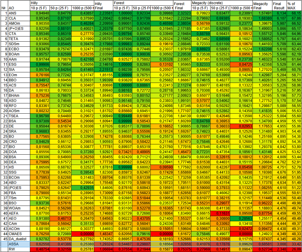
Figure 2. Color coding of algorithms for the corresponding tests

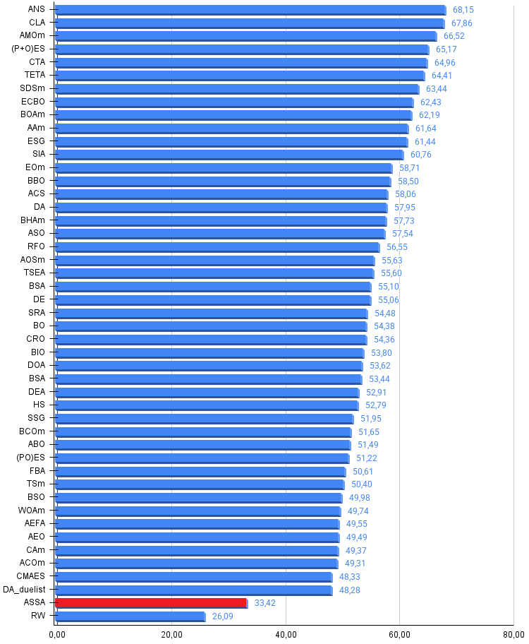
Figure 3. Histogram of algorithm test results (on a scale from 0 to 100; the higher the score, the better, where 100 is the maximum possible theoretical result; the archive contains a script for calculating the ranking table)

Pros and Cons of the ASSA Algorithm

Pros:

1. Few parameters.

Cons:

1. Prone to stagnation.

An archive containing the latest versions of the algorithm code is attached to the article. The author of this article does not assume responsibility for the absolute accuracy of the descriptions of canonical algorithms; many of them have been modified to improve their search capabilities. The conclusions and judgments presented in the articles are based on the results of the experiments conducted.

• GitHub: https://github.com/JQSakaJoo/Population-optimization-algorithms-MQL5

Programs used in this article

#	Name	Type	Description
1	#C_AO.mqh	Include file	Base class for population-based optimization algorithms
2	#C_AO_enum.mqh	Include file	Enumeration of population-based optimization algorithms
3	TestFunctions.mqh	Include file	Test function library
4	TestStandFunctions.mqh	Include file	Test bench function library
5	Utilities.mqh	Include file	Auxiliary functions library
6	CalculationTestResults.mqh	Include file	Script for calculating results for a comparison table
7	Testing AOs.mq5	Script	Unified test bench for all population-based optimization algorithms
8	Simple use of population optimization algorithms.mq5	Script	Simple example of using population-based optimization algorithms without visualization
9	Test_ASSA.mq5	Script	Test bench for ASSA