

Beetle Swarm Optimization (BSO)
 104
104
 0
0

Table of Contents
Introduction
Let's explore another modern optimization algorithm that draws inspiration from nature. Longhorn beetles (Cerambycidae) are one of the largest families of beetles, comprising more than 35,000 species. Their distinctive feature is their extremely long antennae, which often exceed their body length by three to four times. These antennae are not just for show: they constitute an extremely complex sensory system that combines chemoreception, mechanoreception, and even elements of hearing. Beetles use their antennae to find food, locate mates, choose egg-laying sites, and avoid predators. Essentially, the longhorn beetle is a living navigator that continuously “probes” its surroundings by comparing the intensity of chemical gradients on its right and left antennae and turns toward the stronger signal.
It is precisely this principle of two-antenna search that forms the basis of the BAS (Beetle Antennae Search) algorithm proposed by X. Jiang and co-authors. The BAS concept is elegant: a single virtual beetle moves through the solution space, extending its “right” and “left” antennae on either side of its current position. By comparing the values of the objective function at points corresponding to the tips of its antennae, the beetle determines the direction of improvement and takes a step. The algorithm does not require gradient calculations, works with functions of arbitrary form, and is extremely simple — it has only one individual.
However, it was precisely BAS's simplicity that proved to be its limitation. The single-agent approach is highly dependent on the initial position, easily gets stuck in local optima, and performs poorly on multidimensional landscapes where the objective function has a non-uniform structure. These observations led the researchers to the next logical step — combining the BAS antenna mechanism with the collective dynamics of a particle swarm (PSO). This gave rise to the BSO algorithm: Beetle Swarm Optimization.
Beetle Swarm Optimization Algorithm expands the population to a group of beetles, each of which retains the two-antenna detection mechanism but exchanges information with its peers according to rules borrowed from PSO. Each beetle’s position is updated as a weighted combination of two components: the PSO component guides the beetle toward the personal and global best solutions, while the BAS component adjusts its movement based on the local gradient estimated by a pair of antennae. The coefficient "λ" governs the balance between the swarm's "social knowledge" and each individual's "personal perception."
In this article, we will examine the mathematical framework of the BSO algorithm, break down all the key formulas, and present detailed pseudocode and an implementation in MQL5 within the standard test bench for comparing metaheuristic algorithms.
Implementation of the Algorithm
Imagine a clearing filled with a variety of scents. A lone longhorn beetle, with its long antennae extended, is trying to find the source of the strongest scent. It turns its head: if its right antenna detects a stronger scent than the left one, the beetle turns to the right, and vice versa. That is the essence of the BAS algorithm — one scout, two "sensors," and a simple rule.
Now imagine that an entire colony of beetles has emerged into the clearing. Each beetle still senses its surroundings with its antennae, but now they can navigate not only by their own senses — they notice where their fellow beetles are heading, remember their best finds, and know about the colony’s best find. That is BSO — Beetle Swarm Optimization.
The population consists of "n" beetles in an S-dimensional search space. The i-th beetle is described by:
- position Xi = (x_i1, x_i2, …, x_iS) — a point in the solution space,
- velocity Vi = (v_i1, v_i2, …, v_iS) — the direction and magnitude of motion,
- personal best Pi — the best position that this beetle has ever visited,
- global best Pg — the best position found by any beetle in the colony.
Suppose we are looking for the maximum of the function f(x, y) on a plane (S = 2), and we have 3 beetles (n = 3). Initial state:
Beetle; Position X;Velocity V;f(X)
1 (2.0, 3.0) (0.5, -0.3) 7.2
2 (5.0, 1.0) (-0.2, 0.4) 4.8
3 (1.0, 4.0) (0.3, 0.1) 8.5
Each beetle's personal best Pi matches its current position (first iteration). The global best Pg = (1.0, 4.0) with f = 8.5 (beetle No. 3).
Step 1. Each beetle extends its right and left antennae a distance of d/2 from its current position. The direction of the antennae is determined by the beetle's normalized velocity vector — the antennae are aligned along the line of motion.
Antenna positions (formula 10 in the article):
- Xrs = X + V · d/2 (right antenna)
- Xls = X - V · d/2 (left antenna)
Example for beetle No. 1 (X = (2.0, 3.0), V = (0.5, -0.3), d = 0.5):
- Xrs = (2.0 + 0.5·0.25, 3.0 + (-0.3)·0.25) = (2.125, 2.925)
- Xls = (2.0 - 0.5·0.25, 3.0 - (-0.3)·0.25) = (1.875, 3.075)
The beetle probes at two points. Suppose that f(Xrs) = 7.0 and f(Xls) = 7.6. The left antenna found the better value.
Step 2. The BAS increment ξ is computed from the difference between the fitness values at the antennae (formula 9): ξ = δ · V · sign(f(Xrs) - f(Xls))
The "sign" function returns: +1 if the right antenna is better; -1 if the left one is better; 0 if they are equally good.
Continuation of the example for beetle No. 1 (δ = 1.0): sign(7.0 - 7.6) = sign(-0.6) = -1
- ξx = 1.0 · 0.5 · (-1) = -0.5
- ξy = 1.0 · (-0.3) · (-1) = 0.3
A negative value for “x” and a positive value for “y”—the beetle realized it needed to move toward its left antenna (where the scent was stronger), that is, to decrease “x” and increase “y.”
Step 3. The PSO mechanism operates simultaneously: the velocity is updated to account for inertia and the attraction toward the personal best and the global best (Equation 7):
Vnew = ω · V + c₁ · r₁ · (Pi - X) + c₂ · r₂ · (Pg - X); where:
- ω — inertia weight (the extent to which the beetle remembers its previous direction),
- c₁, c₂ — cognitive and social coefficients,
- r₁, r₂ are random numbers in [0, 1].
Continuation of the example for beetle No. 1 (ω = 0.8, c₁ = 1.5, c₂ = 1.5, r₁ = 0.6, r₂ = 0.4):
Personal best P1 = (2.0, 3.0), global best Pg = (1.0, 4.0).
- Vnewx = 0.8·0.5 + 1.5·0.6·(2.0-2.0) + 1.5·0.4·(1.0-2.0) = 0.4 + 0 + (-0.6) = -0.2
- Vnewy = 0.8·(-0.3) + 1.5·0.6·(3.0-3.0) + 1.5·0.4·(4.0-3.0) = -0.24 + 0 + 0.6 = 0.36
Step 4. The new position is calculated as the sum of the current position, the PSO component, and the BAS component with the balance coefficient "λ" (Equation 6):
Xnew = X + λ · Vnew + (1 - λ) · ξ
The parameter λ ∈ [0, 1] controls the contribution of each mechanism:
- λ = 1 — pure PSO (antennae are ignored),
- λ = 0 — pure BAS (swarm intelligence is ignored),
Continuation of the example for beetle No. 1 (λ = 0.5):
- Xnewx = 2.0 + 0.5·(-0.2) + 0.5·(-0.5) = 2.0 - 0.1 - 0.25 = 1.65
- Xnewy = 3.0 + 0.5·0.36 + 0.5·0.3 = 3.0 + 0.18 + 0.15 = 3.33
Xnew = (1.65, 3.33)
The beetle moved from (2.0, 3.0) to (1.65, 3.33) — closer to the global optimum. Both mechanisms agreed that the beetle should move left and upward, and their combination produced a confident step.
Step 5. During the optimization process, two key parameters are adjusted automatically.
The inertia weight "ω" decreases linearly (Equation 8):
ω = ωmax - (ωmax - ωmin) / K · k, where K is the total number of iterations and k is the current iteration.
Example for K = 100:
- k = 1: ω = 0.9 - 0.5/100·1 = 0.895 (broad exploration),
- k = 50: ω = 0.9 - 0.5/100·50 = 0.65 (moderate motion),
- k = 100: ω = 0.9 - 0.5/100·100 = 0.4 (fine-tuning).
A high "ω" at the beginning allows the beetles to quickly spread out across the space, while a low "ω" at the end allows them to thoroughly explore the vicinity of the best solution they have found.
The antenna step size "δ" decays exponentially (Equation 4):
δ^(k+1) = η · δ^k, where η ≈ 0.95
and the distance between the antennae is proportional to the step size (Equation 5):
d = δ / c₂
Example for δ₀ = 1.0, η = 0.95:
- k = 0: δ = 1.0, d = 0.5 (antennae widely spaced),
- k = 20: δ = 0.95²⁰ ≈ 0.358, d ≈ 0.179 (the antennae move closer together),
- k = 60: δ = 0.95⁶⁰ ≈ 0.046, d ≈ 0.023 (fine-grained sniffing).
At the beginning, the beetles probe large regions of the space; at the end, they perform a pointwise analysis. This ensures a smooth transition from global exploration to local exploitation.
Step 6. After evaluating each beetle's new position:
- If f(Xnew) is better than the personal best Pi, update Pi.
- If f(Xnew) is better than the global best Pg, update Pg.
Example. Beetle No. 1 moved to (1.65, 3.33) and obtained a fitness of f = 8.9. This is better than its previous personal best (7.2) and better than the global best (8.5). We update both: P1 = (1.65, 3.33), Pg = (1.65, 3.33). Now all the beetles in the colony know about the new best solution and will be drawn to it.
Summary table of BSO algorithm formulas.
| Formula | Description | |
|---|---|---|
| 6 | X^(k+1) = X^k + λ·V^(k+1) + (1-λ)·ξ^k | Position update (PSO + BAS) |
| 7 | V^(k+1) = ω·V^k + c₁·r₁·(P_i - X) + c₂·r₂·(P_g - X) | Velocity update (PSO) |
| 8 | ω = ωmax - (ωmax - ωmin)/K · k | Linear decrease in inertia weight |
| 9 | ξ = δ · V · sign(f(X_rs) - f(X_ls)) | BAS increment (antenna response) |
| 10 | X_rs = X + V·d/2, X_ls = X - V·d/2 | Positions of the right and left antennae |
| 4 | δ^(k+1) = η · δ^k | Exponential step-size decay |
| 5 | d = δ / c₂ | Distance between the antennae |
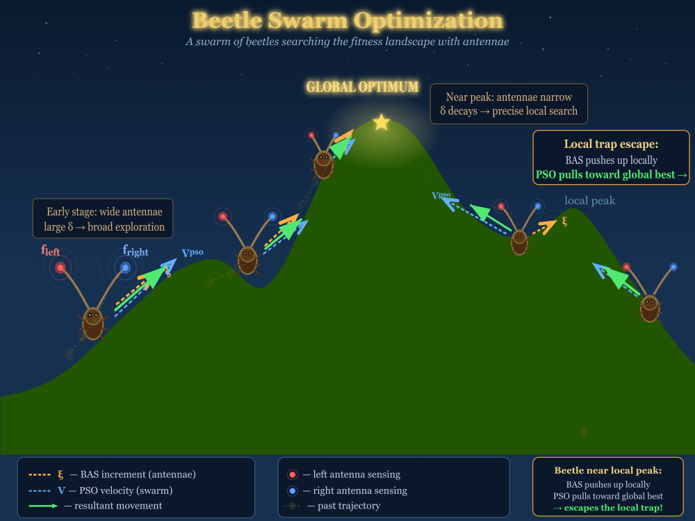
Figure 1. Illustration of the BSO algorithm in action
The illustration depicts a search scene on a hilly fitness landscape: five beetles at different stages of the search — from an early-stage explorer on the left to a beetle near the global peak. Each beetle has visible red (left) and blue (right) antennae with search waves, and the beetle near the peak has antennae that are close together (δ decays). Three types of arrows: an orange dashed ξ arrow (BAS — the antennae indicate the direction), a blue dashed V arrow (PSO — the swarm pulls toward the best position), and a solid green arrow for the resulting movement.
Let's write pseudocode for the BSO algorithm.
n — population size (popSize)
S — dimension of the space (coords)
K_total — total budget for Moving/Revision calls (epochsP)
λ — PSO/BAS balance [0, 1]
c₁, c₂ — cognitive and social PSO coefficients
ω_max, ω_min — inertia weight range
η — step-size decay coefficient (≈ 0.95)
δ₀ — initial BAS step size
c₂_bas — divisor for the distance between the antennae
INITIALIZATION (Init):
For each dimension s = 1..S:
Vmax[s] = (rangeMax[s] − rangeMin[s]) / 2
For each beetle i = 1..n:
cP[i] = random position within the search space // real-valued position
V[i] = random velocity in [−Vmax, Vmax] // initial velocity
δ = δ₀ // current BAS step size
d = δ / c₂_bas // distance between the antennae
K = (K_total − 1) / 3 // number of BSO iterations
k = 0 // iteration counter
phase = −1 // initial phase
MAIN LOOP (alternating Moving → fitness evaluation → Revision):
┌─ Moving (phase = −1):
For each beetle i:
c[i] = discretize(cP[i]) // set positions for evaluation
├─ Revision (phase = −1):
For each beetle i:
cB[i] = c[i], fB[i] = f[i] // personal best = initial position
If f[i] > fB_global:
fB_global = f[i], cB_global = c[i] // update global best
phase = 0
┌─── BSO ITERATION LOOP (repeat while k < K): ───────────────────┐
Moving (phase = 0): // RIGHT ANTENNA
For each beetle i:
c[i] = discretize(cP[i] + V[i] · d/2)
Revision (phase = 0):
For each beetle i:
fR[i] = f[i] // store the fitness for the right antenna
phase = 1
Moving (phase = 1): // LEFT ANTENNA
For each beetle i:
c[i] = discretize(cP[i] − V[i] · d/2)
Revision (phase = 1):
For each beetle i:
fL[i] = f[i] // store the fitness for the left antenna
ω = ω_max − (ω_max − ω_min)/K · (k+1) // formula (8)
ω = max(ω, ω_min) // safety clamp
For each beetle i:
sign = sign(fR[i] − fL[i])
For each dimension s:
ξ = δ · V[i,s] · sign // formula (9)
r₁, r₂ = random numbers from [0, 1]
V[i,s] = ω·V[i,s]
+ c₁·r₁·(cB[i,s] − cP[i,s])
+ c₂·r₂·(cB_global[s] − cP[i,s]) // formula (7)
V[i,s] = clamp(V[i,s], −Vmax[s], Vmax[s])
cP[i,s] = cP[i,s] + λ·V[i,s] + (1−λ)·ξ // formula (6)
cP[i,s] = clamp(cP[i,s], rangeMin[s], rangeMax[s])
δ = η · δ // formula (4)
d = δ / c₂_bas // formula (5)
k = k + 1
phase = 2
Moving (phase = 2): // BEETLE POSITION
For each beetle i:
c[i] = discretize(cP[i])
Revision (phase = 2):
For each beetle i:
If f[i] > fB[i]:
fB[i] = f[i], cB[i] = c[i] // update personal best
If f[i] > fB_global:
fB_global = f[i], cB_global = c[i] // update global best
phase = 0 // start a new iteration
└───────────────────────────────────────────────────────────────────┘
OUTPUT: cB_global, fB_global
Let's move on to the implementation. The C_AO_BSO_Beetle class inherits from the base class C_AO and implements the Beetle Swarm Optimization algorithm — a hybrid of Particle Swarm Optimization (PSO) and Beetle Antennae Search (BAS). Inheritance from C_AO ensures compatibility with the standard test bench: the external code calls Moving() in a loop, then evaluates fitness, then calls Revision(), and the algorithm must fit into this two-stage scheme. A distinctive feature of BSO is that each logical iteration requires three fitness evaluations — for the right antenna, the left antenna, and the beetle’s own position — which is why the implementation uses an internal state machine based on the "phase" variable.
The class contains nine configurable parameters. The "lambda" parameter controls the balance between the PSO component and the BAS component when updating the position: when "lambda" is equal to one, the algorithm becomes pure PSO; when it is zero, it becomes pure BAS; the recommended value is 0.5. The parameters "c1_pso" and "c2_pso" are the cognitive and social PSO coefficients, which determine the strength of attraction to the personal best and the global best solution, respectively. The "omega_max" and "omega_min" parameters specify the range of the linear decay of the inertia weight: at the beginning of optimization, a high inertia weight encourages broad exploration of the space, while at the end, a low inertia weight ensures fine-tuning.
The "eta" parameter is the exponential decay factor for the antenna search step, typically 0.95: at each iteration, the step size "δ" is multiplied by "eta", which gradually narrows the area probed by the antennae. The "delta0" parameter is the initial value of the step size "δ". The "c2_bas" parameter is a divisor that determines the distance between the antennae: d = δ / c2_bas. All parameters are declared in the "public" section and duplicated in the "params" array to ensure consistent access from the test bench.
Four arrays that have no counterparts in the parent class are declared in the "private" section. The "V" array stores the velocities of all beetles across all dimensions in a flat format. The "fR" and "fL" arrays store the fitness values calculated at the right and left antenna positions, respectively — one value per beetle. The "Vmax" array stores the maximum allowable velocity for each dimension, calculated as half the width of the search range.
The "delta" variable stores the current BAS step size, which decreases with each iteration. The "d_ant" variable stores the current distance between the antennae, which is updated in sync with "delta". The "omega" variable stores the current inertia weight, which is recalculated at each BSO iteration. The "phase" variable takes values ranging from minus one to two and determines which action is performed in the current Moving/Revision cycle. The "totalBSOepochs" variable contains the total number of full BSO iterations available within the allocated evaluation budget, while "bsoEpoch" is a counter of the completed iterations.
The "Idx" helper method takes a beetle number and a coordinate number and returns a linear index for accessing the flat velocity array "V". The Clamp method limits the value of "val" to a range between "minV" and "maxV": if the value is less than the minimum, it returns the minimum; if it is greater than the maximum, it returns the maximum; otherwise, it returns the original value.
//————————————————————————————————————————————————————————————————————
class C_AO_BSO_Beetle : public C_AO
{
  public: //----------------------------------------------------------
  ~C_AO_BSO_Beetle () { }
  C_AO_BSO_Beetle ()
  {
    ao_name = "BSO(Beetle)";
    ao_desc = "Beetle Swarm Optimization";
    ao_link = "https://www.mql5.com/en/articles/21292";

    popSize   = 50;
    lambda    = 0.5;
    c1_pso    = 4.0;
    c2_pso    = 1.5;
    omega_max = 0.9;
    omega_min = 0.4;
    eta       = 0.95;
    delta0    = 1.0;
    c2_bas    = 2.0;

    ArrayResize (params, 9);

    params [0].name = "popSize";   params [0].val = popSize;
    params [1].name = "lambda";    params [1].val = lambda;
    params [2].name = "c1";        params [2].val = c1_pso;
    params [3].name = "c2";        params [3].val = c2_pso;
    params [4].name = "omega_max"; params [4].val = omega_max;
    params [5].name = "omega_min"; params [5].val = omega_min;
    params [6].name = "eta";       params [6].val = eta;
    params [7].name = "delta0";    params [7].val = delta0;
    params [8].name = "c2_bas";    params [8].val = c2_bas;
  }

  void SetParams ()
  {
    popSize   = (int)params [0].val;
    lambda    = params      [1].val;
    c1_pso    = params      [2].val;
    c2_pso    = params      [3].val;
    omega_max = params      [4].val;
    omega_min = params      [5].val;
    eta       = params      [6].val;
    delta0    = params      [7].val;
    c2_bas    = params      [8].val;
  }

  bool Init (const double &rangeMinP  [],
             const double &rangeMaxP  [],
             const double &rangeStepP [],
             const int     epochsP = 0);

  void Moving   ();
  void Revision ();

  //------------------------------------------------------------------
  double lambda;    // PSO/BAS balance [0,1]
  double c1_pso;    // PSO cognitive coefficient
  double c2_pso;    // PSO social coefficient
  double omega_max; // maximum inertia weight
  double omega_min; // minimum inertia weight
  double eta;       // BAS step attenuation coefficient
  double delta0;    // initial BAS step size
  double c2_bas;    // d = delta / c2_bas

  private: //---------------------------------------------------------
  double V    [];    // beetle velocities [popSize * coords]
  double fR   [];    // fitness of the right antenna [popSize]
  double fL   [];    // fitness of the left antenna [popSize]
  double Vmax [];    // max velocity [coords]

  double delta;
  double d_ant;
  double omega;

  int    phase;
  int    totalBSOepochs;
  int    bsoEpoch;

  int Idx (int i, int c) { return i * coords + c; }

  double Clamp (double val, double minV, double maxV)
  {
    if (val < minV) return minV;
    if (val > maxV) return maxV;
    return val;
  }
};
//————————————————————————————————————————————————————————————————————
The Init method takes arrays of search bounds "rangeMinP", "rangeMaxP", and discretization steps "rangeStepP", as well as an integer "epochsP" — the number of Moving calls that will be made during the entire optimization cycle. First, StandardInit is called from the parent class, which initializes the random number generator, stores the dimension of the space, creates an array of agents of size "popSize", and calls S_AO_Agent::Init for each agent, setting their fitness values to negative infinity and allocating memory for the coordinate arrays.
After standard initialization, the method allocates memory for four custom arrays: "V" with a size of (popSize * coords), "fR" and "fL" with a size of "popSize", and "Vmax" with a size of "coords". It then calculates the maximum velocities: for each dimension, "Vmax" is equal to half the width of the search range.
Next, for each beetle, a random initial position (a[i].cP) is generated within the search domain, and a random initial velocity "V" is generated within the range from -"Vmax" to +"Vmax". The a[i].fB fields have already been set to negative infinity by the call to S_AO_Agent::Init, so no additional initialization is required.
The initial step size "delta" is set to "delta0", and the distance between the antennae "d_ant" is set to (delta / c2_bas). The total number of BSO iterations is calculated using the formula (epochsP − 1) / 3: one is subtracted because the first call to Moving/Revision is used for the initialization phase (phase = −1), and each complete BSO iteration requires three calls (phases 0, 1, and 2). If the result is less than one, it is forcibly set to one. The "bsoEpoch" counter is reset to zero, and "phase" is set to negative one.
//————————————————————————————————————————————————————————————————————
bool C_AO_BSO_Beetle::Init (const double &rangeMinP  [],
                            const double &rangeMaxP  [],
                            const double &rangeStepP [],
                            const int     epochsP = 0)
{
  if (!StandardInit (rangeMinP, rangeMaxP, rangeStepP)) return false;

  //--- custom arrays (only those not present in the parent class)
  ArrayResize (V,    popSize * coords);
  ArrayResize (fR,   popSize);
  ArrayResize (fL,   popSize);
  ArrayResize (Vmax, coords);

  //--- Vmax ---------------------------------------------------------
  for (int c = 0; c < coords; c++)
  {
    Vmax [c] = (rangeMax [c] - rangeMin [c]) * 0.5;
  }

  //------------------------------------------------------------------
  for (int i = 0; i < popSize; i++)
  {
    for (int c = 0; c < coords; c++)
    {
      a [i].cP [c]   = u.RNDfromCI (rangeMin [c], rangeMax [c]);
      V [Idx (i, c)] = u.RNDfromCI (-Vmax [c], Vmax [c]);
    }
  }

  //--- BAS parameters ------------------------------------------------
  delta = delta0;
  d_ant = delta / c2_bas;

  //--- BSO iteration count -----------------------------------------
  totalBSOepochs = (epochsP - 1) / 3;
  if (totalBSOepochs < 1) totalBSOepochs = 1;
  bsoEpoch = 0;

  phase = -1;

  return true;
}
//————————————————————————————————————————————————————————————————————
The Moving method is called by external code to obtain the coordinates at which the fitness is to be calculated. The behavior of the method is entirely determined by the current phase.
In phase -1, the initial placement is performed: for each beetle, the coordinates from "cP" are discretized using the "SeInDiSp" function and stored in (a[i].c). The "SeInDiSp" function maps a continuous value to the nearest valid grid step within the bounds, ensuring compatibility with problems where parameters take discrete values.
In phase 0, the positions of the right antennae are calculated using equation (10): for each beetle and each dimension, the coordinate of the right antenna is equal to (cP + V * d_ant / 2). The result is discretized and stored in (a[i].c). The "SeInDiSp" function automatically clamps the value to the permissible range, so an additional "Clamp" is not required.
In phase 1, the positions of the left antennae are calculated in the same way: the coordinate is equal to (cP − V * d_ant / 2). The result is discretized and stored in (a[i].c).
In phase 2, the updated positions of the beetles from "cP" are discretized and stored in (a[i].c) for the final fitness evaluation. The code for phases -1 and 2 is identical: both copy "cP" → c via discretization, but they are executed at different points in the execution flow.
//————————————————————————————————————————————————————————————————————
void C_AO_BSO_Beetle::Moving ()
{
  //--- PHASE -1: initial positions from cP → c for the first evaluation -------
  if (phase == -1)
  {
    for (int i = 0; i < popSize; i++)
    {
      for (int c = 0; c < coords; c++)
      {
        a [i].c [c] = u.SeInDiSp (a [i].cP [c], rangeMin [c], rangeMax [c], rangeStep [c]);
      }
    }
    return;
  }

  //--- PHASE 0: right antenna — X_rs = cP + V * d/2 -----------------
  if (phase == 0)
  {
    for (int i = 0; i < popSize; i++)
    {
      for (int c = 0; c < coords; c++)
      {
        double xrs = a [i].cP [c] + V [Idx (i, c)] * d_ant / 2.0;
        a [i].c [c] = u.SeInDiSp (xrs, rangeMin [c], rangeMax [c], rangeStep [c]);
      }
    }
    return;
  }

  //--- PHASE 1: left antenna — X_ls = cP - V * d/2 ------------------
  if (phase == 1)
  {
    for (int i = 0; i < popSize; i++)
    {
      for (int c = 0; c < coords; c++)
      {
        double xls = a [i].cP [c] - V [Idx (i, c)] * d_ant / 2.0;
        a [i].c [c] = u.SeInDiSp (xls, rangeMin [c], rangeMax [c], rangeStep [c]);
      }
    }
    return;
  }

  //--- PHASE 2: beetle positions — cP → c for evaluation --------------------
  if (phase == 2)
  {
    for (int i = 0; i < popSize; i++)
    {
      for (int c = 0; c < coords; c++)
      {
        a [i].c [c] = u.SeInDiSp (a [i].cP [c], rangeMin [c], rangeMax [c], rangeStep [c]);
      }
    }
    return;
  }
}
//————————————————————————————————————————————————————————————————————
The Revision method is called after the external code has calculated the fitness at the coordinates set in Moving. Behavior is determined by the current phase.
In phase minus one, a one-time initial processing step is performed: for each beetle, the fitness of the initial position (a[i].f) is written to (a[i].fB), and the discretized coordinates (a[i].c) are copied to (a[i].cB) — this is how the initial personal bests are formed. At the same time, it checks whether the current fitness is better than the global best fitness, "fB," and updates "fB" and "cB" if necessary. After all the beetles have been processed, "phase" switches to zero — the main loop begins.
In phase zero, the value (a[i].f) for each beetle is stored in the array "fR" — this is the fitness of the right antennae. No best-position updates take place; antenna fitness must not affect the personal bests or the global best. "Phase" switches to 1.
In phase one, the main computational work of the BSO iteration is performed. First, the fitness of the left antennae (a[i].f) is stored in the array "fL." Next, the inertia weight "omega" is calculated using formula (8): omega = omega_max − (omega_max − omega_min) / totalBSOepochs * (bsoEpoch + 1). bsoEpoch + 1 is used because on the first iteration bsoEpoch is zero, while the formula assumes k ranges from 1 to K. An additional clamp ensures that omega does not fall below omega_min due to rounding errors during division.
Next, for each beetle, the sign of the fitness difference between the right and left antennae is calculated: signVal = sign(fR[i] − fL[i]). If the right antenna produced the better fitness, "signVal" is plus one; if the left antenna did, it is minus one; if they are equal, it is zero. Next, three values are calculated sequentially for each dimension. The BAS increment "xi" is calculated by formula (9): xi = delta * V[idx] * signVal. It is the product of the current step size, the current velocity, and the sign, using the previous values of "V" and "delta" before they are updated. The new velocity "vNew" is calculated by formula (7): vNew = omega * V[idx] + c1_pso * r1 * (a[i].cB[c] − a[i].cP[c]) + c2_pso * r2 * (cB[c] − a[i].cP[c]), where "r1" and "r2" are independent random numbers from the interval [0, 1], a[i].cB[c] is the beetle's personal best position, and cB[c] is the global best position. The velocity is clamped to the range from -"Vmax" to +"Vmax". The new position "xNew" is computed by formula (6): xNew = a [i].cP [c] + lambda * vNew + (1 − lambda) * xi — a weighted sum of the PSO component and the BAS component. The position is clamped to the search boundaries. The updated velocity and position are written back to (V [idx]) and (a [i].cP [c]).
After processing all the beetles, the BAS parameters are damped: "delta" is multiplied by eta according to formula (4), and "d_ant" is recalculated as (delta / c2_bas) according to formula (5). The "bsoEpoch" counter is incremented, and "phase" is set to 2.
In phase two, for each beetle, the system checks whether its fitness has improved compared to its personal best. Please note that the discretized coordinates (a [i].c), not the continuous ones (a [i].cP), are copied into "cB", since the fitness was calculated using the discretized coordinates. The global best is checked in a similar way: if (a [i].f > fB), "fB" and "cB" of the "C_AO" class are updated. "Phase" is reset to zero, starting a new BSO iteration.
The sequence of operations within phase one is critical and cannot be changed. First, the BAS increment "xi" is calculated based on the previous velocity "V" and the previous step size "delta" — this ensures that the antenna signal uses the same direction in which the beetle was moving during probing. Next, the new velocity "vNew" is calculated using the PSO formula with the current "omega". The new position is then calculated as a combination of the old position, the new velocity, and the old BAS increment. Only after all the beetles have been processed are "delta" and "d_ant" damped. If "delta" were to decay before "xi" was computed, or if the velocity were updated before "xi" was computed, the result would be incorrect because the BAS increment must correspond to the same conditions under which the antennae evaluated the fitness.
One complete BSO iteration requires three Moving/Revision calls: phase 0 (right antenna), phase 1 (left antenna + computations), phase 2 (beetle's position). Each Moving call generates "popSize" points for evaluation, so a single BSO iteration consumes 3 * popSize evaluations of the objective function. With a standard budget of 10,000 evaluations and popSize = 50, this results in approximately 66 full BSO iterations — one-third as many as a standard PSO would achieve with the same budget. The additional cost is justified by the fact that the antenna mechanism provides information about the local gradient without numerical differentiation, which allows each step to be more accurate.
//————————————————————————————————————————————————————————————————————
void C_AO_BSO_Beetle::Revision ()
{
  //--- PHASE -1: initialization of personal and global bests -----------
  if (phase == -1)
  {
    for (int i = 0; i < popSize; i++)
    {
      a [i].fB = a [i].f;
      ArrayCopy (a [i].cB, a [i].c, 0, 0, coords);

      if (a [i].f > fB)
      {
        fB = a [i].f;
        ArrayCopy (cB, a [i].c, 0, 0, coords);
      }
    }

    phase = 0;
    return;
  }

  //--- PHASE 0: store the fitness of the right antennae -----------------------
  if (phase == 0)
  {
    for (int i = 0; i < popSize; i++) fR [i] = a [i].f;
    phase = 1;
    return;
  }

  //--- PHASE 1: store the fitness of the left antennae + update ξ, V, cP ----
  if (phase == 1)
  {
    for (int i = 0; i < popSize; i++) fL [i] = a [i].f;

    // Equation (8): ω
    omega = omega_max - (omega_max - omega_min) / (double)totalBSOepochs * (double)(bsoEpoch + 1);
    if (omega < omega_min) omega = omega_min;

    for (int i = 0; i < popSize; i++)
    {
      double signVal = 0.0;
      if (fR [i] > fL [i]) signVal =  1.0;
      else
        if (fR [i] < fL [i]) signVal = -1.0;

      for (int c = 0; c < coords; c++)
      {
        int idx = Idx (i, c);

        // Equation (9): ξ = δ * V * sign(fR - fL)
        double xi = delta * V [idx] * signVal;

        // Equation (7): V_new = ω*V + c1*r1*(cB_i - cP) + c2*r2*(cB_g - cP)
        double r1 = u.RNDfromCI (0.0, 1.0);
        double r2 = u.RNDfromCI (0.0, 1.0);

        double vNew = omega  * V [idx]
                      + c1_pso * r1 * (a [i].cB [c] - a [i].cP [c])
                      + c2_pso * r2 * (cB [c] - a [i].cP [c]);

        vNew = Clamp (vNew, -Vmax [c], Vmax [c]);

        // Equation (6): X_new = X + λ*V_new + (1-λ)*ξ
        double xNew = a [i].cP [c] + lambda * vNew + (1.0 - lambda) * xi;
        xNew = Clamp (xNew, rangeMin [c], rangeMax [c]);

        V [idx] = vNew;
        a [i].cP [c] = xNew;
      }
    }

    // Equation (4): δ = η*δ,  Equation (5): d = δ/c2_bas
    delta = eta * delta;
    d_ant = delta / c2_bas;
    bsoEpoch++;

    phase = 2;
    return;
  }

  //--- PHASE 2: evaluating positions, updating the bests --------------------
  if (phase == 2)
  {
    for (int i = 0; i < popSize; i++)
    {
      if (a [i].f > a [i].fB)
      {
        a [i].fB = a [i].f;
        ArrayCopy (a [i].cB, a [i].c, 0, 0, coords);
      }

      if (a [i].f > fB)
      {
        fB = a [i].f;
        ArrayCopy (cB, a [i].c, 0, 0, coords);
      }
    }

    phase = 0;
    return;
  }
}
//————————————————————————————————————————————————————————————————————
Test Results
The BSO algorithm achieved a score of 43% on the standard test set, which corresponds to the average overall level among most metaheuristics; however, this does not allow it to enter the ranking table, whose lower threshold is above 48%.BSO(Beetle)|Beetle Swarm Optimization|50.0|0.5|4.0|1.5|0.9|0.4|0.95|1.0|2.0|
=============================
5 Hilly's; Func runs: 10000; result: 0.863284721848441
25 Hilly's; Func runs: 10000; result: 0.4419698960521393
500 Hilly's; Func runs: 10000; result: 0.2695211726191594
=============================
5 Forest's; Func runs: 10000; result: 0.8504590892687588
25 Forest's; Func runs: 10000; result: 0.4483586443765045
500 Forest's; Func runs: 10000; result: 0.21373784941636523
=============================
5 Megacity's; Func runs: 10000; result: 0.4338461538461539
25 Megacity's; Func runs: 10000; result: 0.2572307692307692
500 Megacity's; Func runs: 10000; result: 0.11098461538461646
=============================
Overall score: 3.88939 (43.22%)
Visualization of the BSO algorithm in action.

BSO on the Hilly test function

BSO on the Forest test function

BSO on the Megacity test function

BSO on the standard Ackley function

BSO on the standard Rastrigin function
The figure below clearly shows, on our standard test problems, how the algorithm behaves as the number of iterations increases. I decided to show this to demonstrate that even with 100,000 fitness-function evaluations (we usually use 10,000 evaluations in tests), the algorithm gets stuck and does not reach full (100%) convergence.

BSO on standard functions Hilly, Forest, Megacity
Based on the test results, the BSO algorithm is included in our ranking table for informational purposes only.
| No. | AO | Description | Hilly | Hilly Final | Forest | Forest Final | Megacity (discrete) | Megacity Final | Final Result | % of MAX | ||||||
| 10 p (5 F) | 50 p (25 F) | 1,000 p (500 F) | 10 p (5 F) | 50 p (25 F) | 1,000 p (500 F) | 10 p (5 F) | 50 p (25 F) | 1,000 p (500 F) | ||||||||
| 1 | ANS | across neighborhood search | 0.94948 | 0.84776 | 0.43857 | 2.23581 | 1.00000 | 0.92334 | 0.39988 | 2.32323 | 0.70923 | 0.63477 | 0.23091 | 1.57491 | 6.134 | 68.15 |
| 2 | CLA | code lock algorithm (joo) | 0.95345 | 0.87107 | 0.37590 | 2.20042 | 0.98942 | 0.91709 | 0.31642 | 2.22294 | 0.79692 | 0.69385 | 0.19303 | 1.68380 | 6.107 | 67.86 |
| 3 | AMOm | animal migration optimization M | 0.90358 | 0.84317 | 0.46284 | 2.20959 | 0.99001 | 0.92436 | 0.46598 | 2.38034 | 0.56769 | 0.59132 | 0.23773 | 1.39675 | 5.987 | 66.52 |
| 4 | (P+O)ES | (P+O) evolutionary strategies | 0.92256 | 0.88101 | 0.40021 | 2.20379 | 0.97750 | 0.87490 | 0.31945 | 2.17185 | 0.67385 | 0.62985 | 0.18634 | 1.49003 | 5.866 | 65.17 |
| 5 | CTA | comet tail algorithm (joo) | 0.95346 | 0.86319 | 0.27770 | 2.09435 | 0.99794 | 0.85740 | 0.33949 | 2.19484 | 0.88769 | 0.56431 | 0.10512 | 1.55712 | 5.846 | 64.96 |
| 6 | TETA | time evolution travel algorithm (joo) | 0.91362 | 0.82349 | 0.31990 | 2.05701 | 0.97096 | 0.89532 | 0.29324 | 2.15952 | 0.73462 | 0.68569 | 0.16021 | 1.58052 | 5.797 | 64.41 |
| 7 | SDSm | stochastic diffusion search M | 0.93066 | 0.85445 | 0.39476 | 2.17988 | 0.99983 | 0.89244 | 0.19619 | 2.08846 | 0.72333 | 0.61100 | 0.10670 | 1.44103 | 5.709 | 63.44 |
| 8 | ECBO | enhanced_colliding_bodies_optimization | 0.93479 | 0.75747 | 0.32471 | 2.01697 | 0.97436 | 0.77446 | 0.23037 | 1.97919 | 0.88923 | 0.58061 | 0.15224 | 1.62208 | 5.618 | 62.43 |
| 9 | BOAm | billiards optimization algorithm M | 0.95757 | 0.82599 | 0.25235 | 2.03590 | 1.00000 | 0.90036 | 0.30502 | 2.20538 | 0.73538 | 0.52523 | 0.09563 | 1.35625 | 5.598 | 62.19 |
| 10 | AAm | archery algorithm M | 0.91744 | 0.70876 | 0.42160 | 2.04780 | 0.92527 | 0.75802 | 0.35328 | 2.03657 | 0.67385 | 0.55200 | 0.23738 | 1.46323 | 5.548 | 61.64 |
| 11 | ESG | evolution of social groups (joo) | 0.99906 | 0.79654 | 0.35056 | 2.14616 | 1.00000 | 0.82863 | 0.13102 | 1.95965 | 0.82333 | 0.55300 | 0.04725 | 1.42358 | 5.529 | 61.44 |
| 12 | SIA | simulated isotropic annealing (joo) | 0.95784 | 0.84264 | 0.41465 | 2.21513 | 0.98239 | 0.79586 | 0.20507 | 1.98332 | 0.68667 | 0.49300 | 0.09053 | 1.27020 | 5.469 | 60.76 |
| 13 | EOm | extremal_optimization_M | 0.76166 | 0.77242 | 0.31747 | 1.85155 | 0.99999 | 0.76751 | 0.23527 | 2.00277 | 0.74769 | 0.53969 | 0.14249 | 1.42987 | 5.284 | 58.71 |
| 14 | BBO | biogeography-based optimization | 0.94912 | 0.69456 | 0.35031 | 1.99399 | 0.93820 | 0.67365 | 0.25682 | 1.86867 | 0.74615 | 0.48277 | 0.17369 | 1.40261 | 5.265 | 58.50 |
| 15 | ACS | artificial cooperative search | 0.75547 | 0.74744 | 0.30407 | 1.80698 | 1.00000 | 0.88861 | 0.22413 | 2.11274 | 0.69077 | 0.48185 | 0.13322 | 1.30583 | 5.226 | 58.06 |
| 16 | DA | dialectical algorithm | 0.86183 | 0.70033 | 0.33724 | 1.89940 | 0.98163 | 0.72772 | 0.28718 | 1.99653 | 0.70308 | 0.45292 | 0.16367 | 1.31967 | 5.216 | 57.95 |
| 17 | BHAm | black hole algorithm M | 0.75236 | 0.76675 | 0.34583 | 1.86493 | 0.93593 | 0.80152 | 0.27177 | 2.00923 | 0.65077 | 0.51646 | 0.15472 | 1.32195 | 5.196 | 57.73 |
| 18 | ASO | anarchy society optimization | 0.84872 | 0.74646 | 0.31465 | 1.90983 | 0.96148 | 0.79150 | 0.23803 | 1.99101 | 0.57077 | 0.54062 | 0.16614 | 1.27752 | 5.178 | 57.54 |
| 19 | RFO | royal flush optimization (JOO) | 0.83361 | 0.73742 | 0.34629 | 1.91733 | 0.89424 | 0.73824 | 0.24098 | 1.87346 | 0.63154 | 0.50292 | 0.16421 | 1.29867 | 5.089 | 56.55 |
| 20 | AOSm | atomic orbital search M | 0.80232 | 0.70449 | 0.31021 | 1.81702 | 0.85660 | 0.69451 | 0.21996 | 1.77107 | 0.74615 | 0.52862 | 0.14358 | 1.41835 | 5.006 | 55.63 |
| 21 | TSEA | turtle shell evolution algorithm (JOO) | 0.96798 | 0.64480 | 0.29672 | 1.90949 | 0.99449 | 0.61981 | 0.22708 | 1.84139 | 0.69077 | 0.42646 | 0.13598 | 1.25322 | 5.004 | 55.60 |
| 22 | BSA | backtracking_search_algorithm | 0.97309 | 0.54534 | 0.29098 | 1.80941 | 0.99999 | 0.58543 | 0.21747 | 1.80289 | 0.84769 | 0.36953 | 0.12978 | 1.34700 | 4.959 | 55.10 |
| 23 | DE | differential evolution | 0.95044 | 0.61674 | 0.30308 | 1.87026 | 0.95317 | 0.78896 | 0.16652 | 1.90865 | 0.78667 | 0.36033 | 0.02953 | 1.17653 | 4.955 | 55.06 |
| 24 | SRA | successful restaurateur algorithm (JOO) | 0.96883 | 0.63455 | 0.29217 | 1.89555 | 0.94637 | 0.55506 | 0.19124 | 1.69267 | 0.74923 | 0.44031 | 0.12526 | 1.31480 | 4.903 | 54.48 |
| 25 | BO | bonobo_optimizer | 0.77565 | 0.63805 | 0.32908 | 1.74278 | 0.88088 | 0.76344 | 0.25573 | 1.90005 | 0.61077 | 0.49846 | 0.14246 | 1.25169 | 4.895 | 54.38 |
| 26 | CRO | chemical reaction optimization | 0.94629 | 0.66112 | 0.29853 | 1.90593 | 0.87906 | 0.58422 | 0.21146 | 1.67473 | 0.75846 | 0.42646 | 0.12686 | 1.31178 | 4.892 | 54.36 |
| 27 | BIO | blood inheritance optimization (JOO) | 0.81568 | 0.65336 | 0.30877 | 1.77781 | 0.89937 | 0.65319 | 0.21760 | 1.77016 | 0.67846 | 0.47631 | 0.13902 | 1.29378 | 4.842 | 53.80 |
| 28 | DOA | dream_optimization_algorithm | 0.85556 | 0.70085 | 0.37280 | 1.92921 | 0.73421 | 0.48905 | 0.24147 | 1.46473 | 0.77231 | 0.47354 | 0.18561 | 1.43146 | 4.825 | 53.62 |
| 29 | BSA | bird swarm algorithm | 0.89306 | 0.64900 | 0.26250 | 1.80455 | 0.92420 | 0.71121 | 0.24939 | 1.88479 | 0.69385 | 0.32615 | 0.10012 | 1.12012 | 4.809 | 53.44 |
| 30 | DEA | dolphin_echolocation_algorithm | 0.75995 | 0.67572 | 0.34171 | 1.77738 | 0.89582 | 0.64223 | 0.23941 | 1.77746 | 0.61538 | 0.44031 | 0.15115 | 1.20684 | 4.762 | 52.91 |
| 31 | HS | harmony search | 0.86509 | 0.68782 | 0.32527 | 1.87818 | 0.99999 | 0.68002 | 0.09590 | 1.77592 | 0.62000 | 0.42267 | 0.05458 | 1.09725 | 4.751 | 52.79 |
| 32 | SSG | saplings sowing and growing | 0.77839 | 0.64925 | 0.39543 | 1.82308 | 0.85973 | 0.62467 | 0.17429 | 1.65869 | 0.64667 | 0.44133 | 0.10598 | 1.19398 | 4.676 | 51.95 |
| 33 | BCOm | bacterial chemotaxis optimization M | 0.75953 | 0.62268 | 0.31483 | 1.69704 | 0.89378 | 0.61339 | 0.22542 | 1.73259 | 0.65385 | 0.42092 | 0.14435 | 1.21912 | 4.649 | 51.65 |
| 34 | ABO | african buffalo optimization | 0.83337 | 0.62247 | 0.29964 | 1.75548 | 0.92170 | 0.58618 | 0.19723 | 1.70511 | 0.61000 | 0.43154 | 0.13225 | 1.17378 | 4.634 | 51.49 |
| 35 | (PO)ES | (PO) evolution strategies | 0.79025 | 0.62647 | 0.42935 | 1.84606 | 0.87616 | 0.60943 | 0.19591 | 1.68151 | 0.59000 | 0.37933 | 0.11322 | 1.08255 | 4.610 | 51.22 |
| 36 | FBA | fractal-based algorithm | 0.79000 | 0.65134 | 0.28965 | 1.73099 | 0.87158 | 0.56823 | 0.18877 | 1.62858 | 0.61077 | 0.46062 | 0.12398 | 1.19537 | 4.555 | 50.61 |
| 37 | TSm | tabu search M | 0.87795 | 0.61431 | 0.29104 | 1.78330 | 0.92885 | 0.51844 | 0.19054 | 1.63783 | 0.61077 | 0.38215 | 0.12157 | 1.11449 | 4.536 | 50.40 |
| 38 | BSO | brain storm optimization | 0.93736 | 0.57616 | 0.29688 | 1.81041 | 0.93131 | 0.55866 | 0.23537 | 1.72534 | 0.55231 | 0.29077 | 0.11914 | 0.96222 | 4.498 | 49.98 |
| 39 | WOAm | whale optimization algorithm M | 0.84521 | 0.56298 | 0.26263 | 1.67081 | 0.93100 | 0.52278 | 0.16365 | 1.61743 | 0.66308 | 0.41138 | 0.11357 | 1.18803 | 4.476 | 49.74 |
| 40 | AEFA | artificial electric field algorithm | 0.87700 | 0.61753 | 0.25235 | 1.74688 | 0.92729 | 0.72698 | 0.18064 | 1.83490 | 0.66615 | 0.11631 | 0.09508 | 0.87754 | 4.459 | 49.55 |
| 41 | AEO | artificial ecosystem-based optimization algorithm | 0.91380 | 0.46713 | 0.26470 | 1.64563 | 0.90223 | 0.43705 | 0.21400 | 1.55327 | 0.66154 | 0.30800 | 0.28563 | 1.25517 | 4.454 | 49.49 |
| 42 | CAm | camel algorithm M | 0.78684 | 0.56042 | 0.35133 | 1.69859 | 0.82772 | 0.56041 | 0.24336 | 1.63149 | 0.64846 | 0.33092 | 0.13418 | 1.11356 | 4.444 | 49.37 |
| 43 | ACOm | ant colony optimization M | 0.88190 | 0.66127 | 0.30377 | 1.84693 | 0.85873 | 0.58680 | 0.15051 | 1.59604 | 0.59667 | 0.37333 | 0.02472 | 0.99472 | 4.438 | 49.31 |
| 44 | CMAES | covariance_matrix_adaptation_evolution_strategy | 0.76258 | 0.72089 | 0.00000 | 1.48347 | 0.82056 | 0.79616 | 0.00000 | 1.61672 | 0.75846 | 0.49077 | 0.00000 | 1.24923 | 4.349 | 48.33 |
| 45 | DA_duelist | duelist_algorithm | 0.92782 | 0.53778 | 0.27792 | 1.74352 | 0.86957 | 0.47536 | 0.18193 | 1.52686 | 0.62153 | 0.33569 | 0.11715 | 1.07437 | 4.345 | 48.28 |
| BSO_beetle | beetle_swarm_optimization | 0.86328 | 0.44196 | 0.26952 | 1.57476 | 0.85045 | 0.44836 | 0.21373 | 1.51254 | 0.43384 | 0.25723 | 0.11098 | 0.80205 | 3.889 | 43.22 | |
| RW | random walk | 0.48754 | 0.32159 | 0.25781 | 1.06694 | 0.37554 | 0.21944 | 0.15877 | 0.75375 | 0.27969 | 0.14917 | 0.09847 | 0.52734 | 2.348 | 26.09 | |
Conclusions
The main idea of BSO — combining the collective intelligence of a swarm (PSO) with local probing by antennae (BAS) — looks attractive at the conceptual level. The two mechanisms do indeed complement each other: PSO provides global orientation, while antenna search adds information about the local gradient without numerical differentiation. However, the practical implementation of this symbiosis has revealed a number of limitations.
The main structural problem is threefold budget consumption. Each BSO iteration consumes three objective-function evaluations per agent (right antenna, left antenna, beetle position). The additional information from the antennae does not compensate for the threefold reduction in the number of iterations — each step is more accurate, but there are too few steps for full convergence.
The convergence analysis revealed a characteristic pattern of stagnation toward the end of the optimization process. Exponential decay of the step size "δ" with a coefficient of η = 0.95 results in "δ" decreasing by a factor of approximately 13 by the 50th iteration, while the distance between the antennae decreases to values at which the fitness difference between the right and left antennae becomes negligibly small. The BAS increment "ξ" is effectively reduced to zero, and the algorithm degenerates into PSO with a reduced budget. Moreover, when "δ" is small, even a formally nonzero "ξ" is so small that its contribution is suppressed by the PSO component. Thus, the antenna mechanism, which is at the heart of the algorithm, operates primarily during the initial iterations and fades away well before the optimization is complete.
There is some variation in the results on low-dimensional test functions. This is due to a combination of factors: a small number of iterations (due to threefold budget consumption), the dependence of the sign function sign(fR − fL) on stochastic fluctuations in the fitness of the antennae, and the high sensitivity of the BAS component to the direction of the velocity vector — with a small number of dimensions, each velocity component makes a significant contribution, and an error in determining the direction from the antennae has a greater impact on the trajectory.
The "λ" parameter, which controls the balance between PSO and BAS, is a key characteristic but one that is difficult to tune. When λ = 1, the algorithm becomes PSO with threefold budget consumption (the worst-case scenario); when λ = 0, it becomes a swarm of independent BAS agents without collective information exchange (which is also inefficient). The optimal value depends on the landscape of the objective function and cannot be determined in advance, which reduces the algorithm's robustness on heterogeneous test sets.
It should be noted that BSO has the potential for modifications: adaptive control of "λ" depending on the search stage, a slower decay of "δ," or a hybrid strategy in which antenna evaluations are performed periodically rather than at every iteration — all of which could improve efficiency. However, in the baseline version described in the original article, the algorithm demonstrates average performance.
BSO ranks near the bottom of the rating table with a score of 43%, placing it on par with other algorithms whose original concepts are interesting but whose practical effectiveness is limited by their design characteristics.
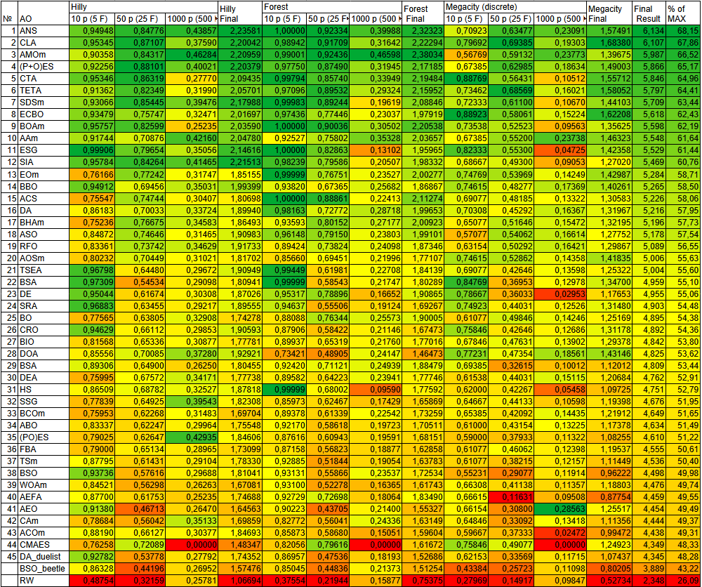
Figure 2. Color gradation of algorithms by the corresponding tests
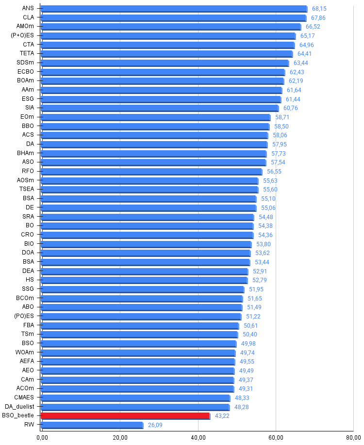
Figure 3. Histogram of the algorithm test results (on a scale from 0 to 100; the higher the score, the better, where 100 is the maximum possible theoretical result; the archive contains a script for calculating the rating table)
Pros and cons of the BSO_beetle algorithm:
Pros:
- None found.
Cons:
- A large number of parameters.
- Gets stuck.
An archive with the latest versions of the algorithm code is attached to the article. The author of this article does not guarantee absolute accuracy in the descriptions of the canonical algorithms; many of them have been modified to improve their search capabilities. The conclusions and judgments presented in the articles are based on the results of the experiments conducted.
Programs used in the article
| # | Name | Type | Description |
|---|---|---|---|
| 1 | #C_AO.mqh | Include file | Parent class of population-based optimization algorithms |
| 2 | #C_AO_enum.mqh | Include file | Enumeration of population-based optimization algorithms |
| 3 | TestFunctions.mqh | Include file | Test function library |
| 4 | TestStandFunctions.mqh | Include file | Library of test bench functions |
| 5 | Utilities.mqh | Include file | Utility functions library |
| 6 | CalculationTestResults.mqh | Include file | Script for calculating results for the comparison table |
| 7 | Testing AOs.mq5 | Script | A unified test bench for all population-based optimization algorithms |
| 8 | Simple use of population optimization algorithms.mq5 | Script | A simple example of using population-based optimization algorithms without visualization |
| 9 | Test_BSO_beetle.mq5 | Script | Test bench for BSO_beetle |
Translated from Russian by MetaQuotes Ltd.
Original article: https://www.mql5.com/ru/articles/21292
Warning: All rights to these materials are reserved by MetaQuotes Ltd. Copying or reprinting of these materials in whole or in part is prohibited.
This article was written by a user of the site and reflects their personal views. MetaQuotes Ltd is not responsible for the accuracy of the information presented, nor for any consequences resulting from the use of the solutions, strategies or recommendations described.

 Neural Networks in Trading: Heterogeneity-Informed Meta-Parameter Learning (HimNet)
 Machine Learning in Pure MQL5 (Part 1): Logistic Regression from Scratch with SGD
 Features of Experts Advisors
 Automating Classic Market Methods in MQL5 (Part 7): The Nicolas Darvas Box System

- Free trading apps
- Over 8,000 signals for copying
- Economic news for exploring financial markets
You agree to website policy and terms of use