Isolation Forest: Unsupervised Anomaly Detection, and What It Actually Finds in Price Data

Contents

• Introduction
• Isolation instead of a model of normal
• A generator you can replay
• One isolation tree
• The forest, and the sub-sample that does the work
• What goes in the columns
• The property that decides the whole feature design
• Verification: the same forest, twice
• Real bars, and the nulls that keep the claim honest
• What it flags, and whether that is new information
• Plotting the decision variable
• A gate in front of a strategy
• Why the backtest cannot answer the question it looks like it answers
• Conclusion

Introduction

Trading systems assume the present resembles the past. That assumption fails on rare bars: a gap into a policy announcement, a liquidation cascade, or the first bar of a regime with no precedent. Detecting them is an unsupervised problem, since there is no label column saying which bars were unusual.

Most classical detectors work backwards. They build a model of "normal", a density estimate or a reconstruction error, and flag whatever fits it poorly. In practice that can mean estimating a fourteen-dimensional density from only a few thousand bars before the real question is addressed.

Liu, Ting and Zhou inverted the problem in 2008. Anomalies are few and different, so instead of describing the crowd, cut the space at random and count how many cuts it takes to leave a point on its own. A point among several hundred similar points needs many cuts; a point off on its own needs two or three. That count, averaged over many random trees, is the anomaly score. No density is estimated and nothing is assumed about the shape of the data.

This article implements that idea as a self-contained MQL5 library, verifies it against Python, and evaluates it on market data and null models. The testing matters as much as the code, because an unsupervised detector always produces output: feed it a random walk and it will faithfully report that walk's most unusual bars.

On 2398 rows of XAUUSD D1 with fourteen feature columns, growing a hundred trees takes 2.4 milliseconds. Scoring all rows adds about thirty more, and scoring one additional bar takes 12.4 microseconds. The bars ranked highest are the October 2025 sell-off, the gold crash of 11 August 2020 and three COVID sessions; on BTCUSD D1 the worst bar in seven years is Black Thursday. The score is not a repackaged z-score, its rank correlation with an absolute normalized return ranking being 0.37, and the calibrated threshold transfers: a cut at the training 95th percentile flags 6.13 percent of an untouched out-of-sample tail.

Isolation instead of a model of normal

The algorithm rests on one observation about random partitioning. Take a set of points and repeatedly split it: pick a coordinate at random, pick a value at random inside that coordinate's range, and send the points either side. Keep going until a point is alone. The number of splits that took is the point's path length.

Points buried in a dense region survive many splits, because almost every random cut lands with points on both sides, while a point far from the rest is separated early. Path length therefore measures directly how easy a point was to isolate.

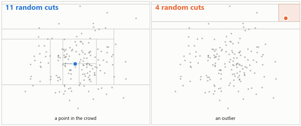
Fig. 1. Random cutting applied to a point in the crowd and to an outlier, with the cut count for each

Two practical problems stand between that idea and a usable number. The first is that growing a tree until every point is alone makes it enormous, and the points needing the deepest trees are the ordinary ones nobody is asking about. So growth stops at a height limit of ceil(log2(psi)), the average depth of a balanced tree over a sub-sample of size psi.

That truncation leaves a hole: a branch cut off at the limit still holds points whose real path length was never counted. The paper closes it with the average path length of an unsuccessful search in a binary search tree, exactly the situation those points are in:

c(n) = 2 * (ln(n - 1) + gamma) - 2 * (n - 1) / n

where gamma is the Euler-Mascheroni constant, about 0.5772. The second problem is that a raw path length depends on how much data the tree saw; dividing by c(psi) removes that dependence and the exponential bounds the result:

s(x) = 2 ^ ( -E[h(x)] / c(psi) )

A point isolated almost immediately scores near 1, a point whose average path length equals c(psi) scores exactly 0.5, and anything buried deeper scores below that.

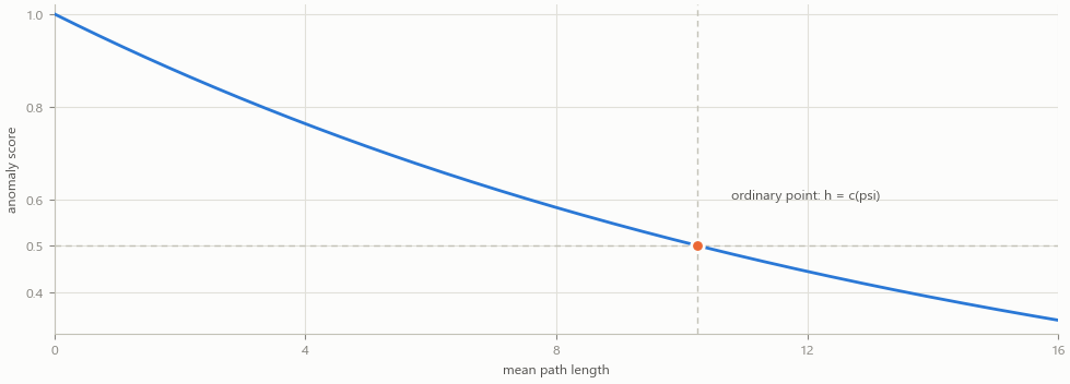
Fig. 2. The score against average path length, hinged at c(psi) where an ordinary point scores one half

Both live in IForestScore.mqh and are the only exact arithmetic in the library:

//+------------------------------------------------------------------+
//| c(n), the average unsuccessful search depth of a BST             |
//+------------------------------------------------------------------+
static double CIForestScore::AveragePathLength(const int n)
  {
   if(n <= 1)
      return(0.0);
   if(n == 2)
      return(1.0);
   double harmonic = MathLog((double)n - 1.0) + IFOREST_EULER_GAMMA;
   return(2.0 * harmonic - 2.0 * ((double)n - 1.0) / (double)n);
  }
//+------------------------------------------------------------------+
//| s(x) = 2^(-E[h(x)] / c(psi))                                     |
//+------------------------------------------------------------------+
static double CIForestScore::Anomaly(const double meanPath, const int psi)
  {
   double norm = AveragePathLength(psi);
   if(norm <= 0.0)
      return(0.0);
   return(MathPow(2.0, -meanPath / norm));
  }

The two early returns are not padding. A node holding one point has no unsearched subtree, so its correction is zero, and a node holding two needs exactly one more comparison. Getting either wrong shifts every score by a constant.

A generator you can replay

Isolation Forest is built entirely out of random choices, so the generator is part of the algorithm rather than a detail of the implementation. MathRand fails here twice over: it returns 15 bits, so a split point has at most 32768 distinct positions available however finely the data is spread, and MathSrand seeds a state that cannot be read back or set, so a run cannot be replayed. Without replay there is no regression test and no way to compare the MQL5 forest against anything outside the terminal.

The library therefore carries its own generator: splitmix64 to turn a user seed into a well-mixed state, then xorshift64* for the stream itself. Both are pure 64-bit integer arithmetic that wraps on overflow, which is exactly what MQL5's ulong does.

//+------------------------------------------------------------------+
//| Mixes the user seed into the generator state                     |
//+------------------------------------------------------------------+
void CIForestRandom::Seed(const ulong seed)
  {
   ulong z = seed + (ulong)0x9E3779B97F4A7C15;
   z = (z ^ (z >> 30)) * (ulong)0xBF58476D1CE4E5B9;
   z = (z ^ (z >> 27)) * (ulong)0x94D049BB133111EB;
   z = z ^ (z >> 31);
   m_state = (z != 0 ? z : (ulong)0x9E3779B97F4A7C15);
  }
//+------------------------------------------------------------------+
//| One 64-bit draw                                                  |
//+------------------------------------------------------------------+
ulong CIForestRandom::NextU64(void)
  {
   ulong x = m_state;
   x ^= (x >> 12);
   x ^= (x << 25);
   x ^= (x >> 27);
   m_state = x;
   return(x * (ulong)0x2545F4914F6CDD1D);
  }
//+------------------------------------------------------------------+
//| Double in [0,1) built from the top 53 bits                       |
//+------------------------------------------------------------------+
double CIForestRandom::Uniform(void)
  {
   return((double)(NextU64() >> 11) * (1.0 / 9007199254740992.0));
  }

Every hexadecimal constant is cast to ulong deliberately. A 16 digit hex literal has its top bit set and parses as a negative signed long; the bit pattern is identical either way, but only the unsigned type gives the logical right shift the algorithm requires. Uniform then takes the top 53 bits, the width of a double's mantissa, so every value it produces is exactly representable.

One detail in NextInt looks like a mistake and is load bearing:

//+------------------------------------------------------------------+
//| Integer in [0,n)                                                 |
//|                                                                  |
//| The modulo bias is below 2^-32 for any n this library uses, and  |
//| the draw happens even for n <= 1 to keep the stream aligned.     |
//+------------------------------------------------------------------+
int CIForestRandom::NextInt(const int n)
  {
   ulong v = NextU64();
   if(n <= 1)
      return(0);
   return((int)(v % (ulong)n));
  }

The draw happens before the early return, so a call that can only answer zero still advances the state. Skipping it is the obvious optimization and it would be wrong: on a single column matrix every column draw answers zero, and if those consumed nothing the generator would run one value ahead for the rest of the run.

The rule behind that is what the whole verification strategy rests on: the number of values drawn from the generator must depend only on the shape of the work, never on the data. Two implementations can then be fed the same seed and required to agree exactly rather than approximately.

One isolation tree

CIForestTree holds its nodes in five parallel arrays rather than in objects, and a node owns a half-open range of a shared index array partitioned in place, so growing a tree copies no feature data at all. Capacity grows by doubling, because the alternative is quadratic:

//+------------------------------------------------------------------+
//| Grows the node arrays by doubling                                |
//|                                                                  |
//| Resizing by one inside the build loop would make a tree cost     |
//| O(nodes^2); this is the pattern the whole workspace uses.        |
//+------------------------------------------------------------------+
void CIForestTree::EnsureCapacity(const int needed)
  {
   if(needed <= m_capacity)
      return;
   int newCap = (m_capacity == 0 ? 256 : m_capacity);
   while(newCap < needed)
      newCap *= 2;
   ArrayResize(m_feat,  newCap);
   ArrayResize(m_split, newCap);
   ArrayResize(m_left,  newCap);
   ArrayResize(m_right, newCap);
   ArrayResize(m_size,  newCap);
   m_capacity = newCap;
  }

The build uses an explicit LIFO stack instead of recursion, mostly for determinism: both children are created before either is expanded, so node numbering is fixed entirely by the order of draws from the generator. The part of the loop that chooses a split, excerpted from Build:

      //--- One draw picks the starting column, then the scan walks
      //--- forward with wraparound to the first column that actually
      //--- varies here. Redrawing until a varying column turns up
      //--- would consume an unpredictable number of values from the
      //--- stream, which no mirror could follow.
      int    q     = rng.NextInt(cols);
      double vmin  = 0.0;
      double vmax  = 0.0;
      bool   found = false;
      for(int k = 0; k < cols; k++)
        {
         int c = (q + k) % cols;
         double a = X[idx[lo] * cols + c];
         double b = a;
         for(int i = lo + 1; i < hi; i++)
           {
            double v = X[idx[i] * cols + c];
            if(v < a)
               a = v;
            if(v > b)
               b = v;
           }
         if(b > a)
           {
            q     = c;
            vmin  = a;
            vmax  = b;
            found = true;
            break;
           }
        }
      if(!found)
         continue;                    // every column identical -> leaf
      double p = vmin + (vmax - vmin) * rng.Uniform();

The wraparound scan is the rule from the previous section costing something. A node whose drawn column is constant produces no usable split, and redrawing until a varying column appears destroys reproducibility, because the number of values consumed then depends on the data. Drawing once and scanning forward consumes exactly one value per node whatever the data looks like.

Partitioning is a single in-place sweep, and the split value is drawn uniformly between the minimum and maximum inside this node, not across the whole column. That local range makes the procedure adapt as the tree descends, and it decides the entire feature design.

Scoring walks the same arrays:

//+------------------------------------------------------------------+
//| How deep this tree had to go before the point stood alone        |
//|                                                                  |
//| x[] is a flat feature matrix and offset is the start of the row. |
//+------------------------------------------------------------------+
double CIForestTree::PathLength(const double &x[], const int offset) const
  {
   if(m_count <= 0)
      return(0.0);
   int node  = 0;
   int depth = 0;
   while(m_feat[node] != -1)
     {
      node = (x[offset + m_feat[node]] < m_split[node]
              ? m_left[node] : m_right[node]);
      depth++;
     }
   return((double)depth + CIForestScore::AveragePathLength(m_size[node]));
  }

The leaf correction is added here, using the number of training points that reached that leaf. A row being scored is not required to have been part of the tree's training sub-sample, which is what makes out-of-sample scoring possible at all.

The forest, and the sub-sample that does the work

A single random tree says almost nothing. The estimate is the average over many, and CIForestEnsemble grows them from one generator so the whole forest is reproducible from a single seed:

//+------------------------------------------------------------------+
//| Grows the forest over a flat rows x cols feature matrix          |
//+------------------------------------------------------------------+
bool CIForestEnsemble::Fit(const double &X[], const int rows, const int cols)
  {
   m_fitted      = false;
   m_totalNodes  = 0;
   m_psiEff      = 0;
   m_heightLimit = 0;
   m_cols        = cols;
   if(rows < 2 || cols < 1)
     {
      Print("IForestEnsemble::Fit - need at least 2 rows and 1 column");
      return(false);
     }
   if(ArraySize(X) < rows * cols)
     {
      Print("IForestEnsemble::Fit - matrix shorter than rows*cols");
      return(false);
     }
   m_psiEff = (m_psi < rows ? m_psi : rows);
   m_heightLimit = (int)MathCeil(MathLog((double)(m_psiEff > 2 ? m_psiEff : 2))
                                 / MathLog(2.0));
   ArrayResize(m_trees, m_nTrees);
   m_rng.Seed(m_seed);
   for(int t = 0; t < m_nTrees; t++)
     {
      m_rng.Subsample(rows, m_psiEff, m_sub);
      m_trees[t].Clear();
      m_trees[t].Build(X, cols, m_sub, ArraySize(m_sub),
                       m_heightLimit, m_rng, m_idx);
      m_totalNodes += m_trees[t].NodeCount();
     }
   m_fitted = true;
   return(true);
  }

The four fields are cleared before the arguments are checked. Score normalizes by c(psi), so a refit that rejected its arguments and left the previous fit's psi in place would return 1.0 for every row, and "everything is maximally anomalous" is the worst available way to say "there is no model".

Each tree sees a sub-sample of psi rows, and psi is small on purpose. The default of 256 is the part of this algorithm that reads backwards to anyone used to machine learning: more data does not make it better, because giving every tree the whole series invites two named failure modes. Swamping is ordinary points looking isolated because the space is crowded. Masking is the interesting one: a group of similar anomalies stops looking anomalous, because each member now has company and is no longer alone after a few cuts. A small sub-sample rarely draws more than one member of such a group, so the group cannot hide itself.

Measured, the driver of masking is the cluster's density rather than its distance from the bulk. At two percent of rows there is no effect at any distance. At fifteen percent, the decline with growing psi is large and monotone:

Sub-sample size psi	32	64	128	256	2048
AUC, clustered anomalies at 15% of rows	0.9863	0.9371	0.8760	0.8129	0.6443

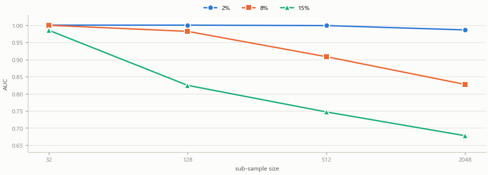
Fig. 3. Masking measured directly: the collapse with growing psi appears only when the anomaly cluster is dense enough to hide in

The table shows the densest case from the shipped test. The figure repeats the same procedure at three densities in a separate run, so its points vary slightly. Fifteen percent is a lot of anomalies, but what both show is that the sub-sampling does real work rather than saving time.

Cost is the other reason psi matters. Growing the forest is O(trees * psi * log psi), with no term for the number of rows at all: a hundred trees over sub-samples of 256 is the same work at two thousand rows or twenty thousand. Scoring is O(trees * log psi) per row, so the row count decides the total cost of a Fit, which scores every training row to calibrate the threshold. Both halves are therefore timed separately with GetMicrosecondCount on an idle terminal, as a minimum over five repeats with the observed range beside it:

XAUUSD, 14 columns, 100 trees, psi 256	grow the trees	+ score every row	per extra bar
2398 daily rows	2.4 ms [2.4-2.9]	32.6 ms [32.6-35.6]	12.4 us
3767 hourly rows	2.5 ms [2.5-3.8]	51.7 ms [51.7-53.5]	12.7 us

The two halves behave as the complexity says. Growing the trees does not move when the history grows by half again; the total does, and the extra 19 milliseconds over the extra 1369 rows comes to 14 microseconds each, within a tenth of the per-bar cost measured independently in the last column. Either way, a refit on every closed bar is nowhere near stalling a chart.

What goes in the columns

Isolation Forest is multivariate and uses one row per bar. The choice of feature columns determines what the library can detect, and CIForestData builds that matrix under two rules. A row for bar i uses bar i and older bars only, with the trailing sigma ending at bar i-1 so a large move cannot inflate the yardstick it is measured against. And a raw price is never a feature, because in a trend every recent bar sits outside the fitted range, and the whole recent history would be flagged for no better reason than that the market went up.

The per-bar feature block, excerpted from the row loop inside Build:

   for(int i = start; i < n; i++)
     {
      //--- trailing statistics over bars i-volWin .. i-1
      double sigma = StdOf(r, i - m_volWin, m_volWin);
      if(sigma <= 0.0)
         continue;
      double atr = MeanOf(span, i - m_volWin, m_volWin);
      int base = m_rows * m_cols;
      int k = 0;
      if(m_mode == IFOREST_MODE_BAR || m_mode == IFOREST_MODE_BOTH)
        {
         m_F[base + k++] = r[i] / sigma;
         m_F[base + k++] = (atr > 0.0 ? span[i] / atr : 0.0);
         m_F[base + k++] = (span[i] > 0.0
                            ? MathAbs(close[i] - open[i]) / span[i] : 0.0);
         if(m_useGap)
            m_F[base + k++] = (open[i] - close[i - 1])
                              / (sigma * close[i - 1]);

Six columns describe the state of one bar: normalized return, range against its trailing average, body as a fraction of range, opening gap, a short cumulative drift, and the ratio of very short to longer volatility. A second mode replaces them with the last d normalized returns, describing the shape of the recent path, and a third concatenates both; the two rank real bars differently, at a rank correlation around 0.45.

The property that decides the whole feature design

Because a split is drawn inside each column's own range, Isolation Forest is exactly invariant to rescaling any single column. That inverts the natural instinct that a column with tiny variance must be a dead column worth dropping: adding uninformative noise columns does the same damage at a spread of 0.015, of 1.0 and of 100. The three rows below are not merely close, they are bit-identical:

Uninformative columns added	0	1	2	3	6	12	24
AUC, noise columns at spread 0.015	0.9155	0.9040	0.8980	0.8608	0.8633	0.7959	0.7514
the same at spread 1.0	0.9155	0.9040	0.8980	0.8608	0.8633	0.7959	0.7514
the same at spread 100	0.9155	0.9040	0.8980	0.8608	0.8633	0.7959	0.7514

What hurts is the count of columns that vary but carry nothing: the first few cost about 0.018 of AUC each in a six-column set, and twenty four cost 0.164 in total. A fitted decision tree evaluates candidate splits and never picks a useless feature; an isolation tree draws its column at random, so every useless column steals draws from the ones that carry signal. There is therefore no automatic dead-column filter here and there cannot be a correct one, because a column being uninformative is not visible in the column itself. Keep the feature set small and deliberate.

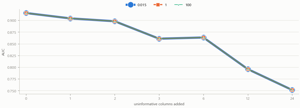
Fig. 4. The table above, plotted: the three spreads land on top of each other, so only the number of empty columns matters

One case is an exception, because it is detectable structurally rather than statistically. On an instrument that trades around the clock there is no jump from previous close to current open, so the gap column carries microstructure noise dressed as a feature. CIForestData therefore reports gap activity, the typical opening jump over the typical one-bar move, and lets the caller decide: XAUUSD D1 reads 0.0506 against BTCUSD D1 at 0.0041.

Verification: the same forest, twice

Verification runs on four levels, and the design goal throughout was to avoid a comparison that can only ever come out approximately right.

The first level covers what is exactly computable: the generator against a reference stream, c(n) against its closed form, the score formula at its hinge, and the structural contract of a tree. The second covers behavior under randomness, where a fixed count would eventually be crossed by an unlucky draw, so every assertion is a ranking statistic or an exact equality. IForest_Test_Detect.mq5 checks that planted anomalies rank above the bulk, that a calibrated 95th percentile leaves five percent above it, that a fixed seed reproduces every score bit for bit, and that the feature matrix cannot see the future.

That last one is worth showing, because a one-bar lookahead is invisible in every summary statistic. The test rewrites one bar mid-series and demands byte-identical rows for every earlier bar:

   double worstBefore = 0.0;
   int    changedAfter = 0;
   for(int r = 0; r < d1.Rows() && r < d2.Rows(); r++)
     {
      int bar = d1.BarOf(r);
      double rowDiff = 0.0;
      for(int col = 0; col < d1.Cols(); col++)
         rowDiff = MathMax(rowDiff, MathAbs(d1.At(r, col) - d2.At(r, col)));
      if(bar < k)
        {
         if(rowDiff > worstBefore)
            worstBefore = rowDiff;
        }
      else
         if(rowDiff > 0.0)
            changedAfter++;
     }

It passes at exactly zero, with 102 later rows correctly moving.

The third level compares against Python, and here the generator pays for itself. MQL5's ulong and Python's integers masked to 64 bits wrap identically, so the two streams match bit for bit and the cross-check becomes an equality rather than a statistical comparison. The MQL5 script exports the bars, the feature matrix, all tree nodes and all scores. Python then rebuilds the forest from the same matrix using the same seed. Across three configurations, zero of two hundred trees differ in structure and every split value matches at 0.000e+00, while an independent vectorized traversal reproduces MQL5's scores to 5.6e-17. Only the feature matrix needs a tolerance, because NumPy sums pairwise where the MQL5 loop sums in order: the worst relative difference is 4.2e-14, always in drift_z, the one feature built by summing several returns.

The fourth comparison is against scikit-learn, and it needs an honest tolerance. The two forests cannot be identical, because different generators make different splits. So the question is whether they land closer than scikit-learn lands to itself when only its seed changes:

Configuration	this library vs scikit-learn	scikit-learn vs itself
14 columns, 100 trees, psi 256	0.9431	0.9306
6 columns, 60 trees, psi 128	0.9365	0.9402
12 columns, 40 trees, psi 64	0.8252	0.8299

Rank agreement, so 1.0 would mean identical orderings. On the fourteen-column case this library sits above scikit-learn's own seed-to-seed floor; on the two smaller ones it sits 0.004 below, which is why the check is a band allowing 0.02 rather than a strict inequality. What would be alarming is a number well outside the spread scikit-learn shows against itself, and there is not one. Note that the floor itself drops to 0.8299 with 40 trees over sub-samples of 64, which is a statement about ensemble size rather than about either implementation.

Level	What it runs	Result
Prototype	iforest_prototype.py self-test	21 PASS, 0 FAIL
Core	IForest_Test_Core.mq5	28 PASS, 0 FAIL
Detection	IForest_Test_Detect.mq5	16 PASS, 0 FAIL
Cross-check	Python rebuild, traversal and scikit-learn	28 PASS, 0 FAIL
Indicator	buffers and panel read back through iCustom	14 PASS, 0 FAIL on two charts

Real bars, and the nulls that keep the claim honest

An unsupervised detector always produces output, so the scan runs the real series and two nulls in the same pass, because they answer different questions.

The weak null is a Gaussian random walk with matched return dispersion. Real markets separate cleanly from it: across ten symbol and timeframe combinations, the real series always has a lower mean score, a higher spread and a higher maximum. Fat tails and volatility clustering produce a handful of extreme bars and a large mass of very quiet ones; a Gaussian walk has neither.

The strong null is more uncomfortable. It shuffles the real bars in time, so each keeps its own return, wick proportions and opening jump, and only the order is destroyed. On XAUUSD D1 the result is close enough to matter:

Series	mean	sd	p50	p95	max
Real XAUUSD D1	0.4077	0.0503	0.3926	0.5114	0.7049
Shuffled bars, run 1	0.3987	0.0406	0.3882	0.4808	0.6840
Shuffled bars, run 2	0.4004	0.0442	0.3883	0.4905	0.6542
Gaussian walk, run 1	0.4573	0.0330	0.4522	0.5192	0.6293
Gaussian walk, run 2	0.4460	0.0368	0.4388	0.5162	0.6218

The shuffled series nearly reproduces the real one, and on BTCUSD D1 the shuffled mean of 0.4131 comes out above the real 0.4072: most of what this forest sees lives in the marginals, not in the time ordering.

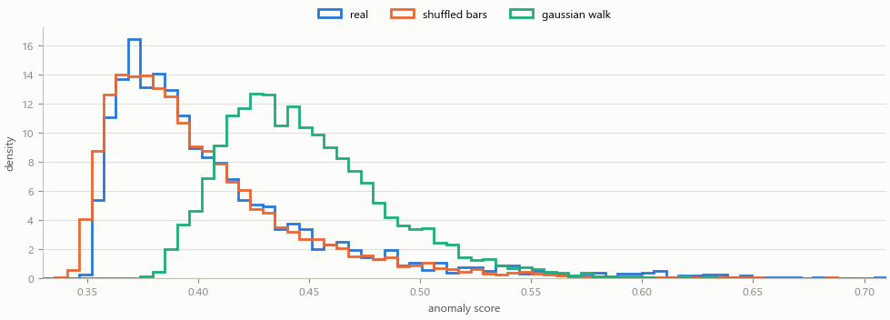
Fig. 5. The Gaussian walk separates from real bars, and the shuffled-bars null almost does not

That does not make the flagged bars wrong; it sets what may honestly be claimed. Any claim of temporal structure has to clear the shuffle null, not the walk.

Important: an anomaly score is a statement about one bar relative to the history the forest was fitted on. It carries no directional content, and reading its level as a market regime meter is not supported by the numbers above.

What it flags, and whether that is new information

The bars ranked highest on XAUUSD D1 are real events, and the feature values beside them explain the ranking:

Date	score	ret_z	range_atr	body_frac	volratio
2025.10.21	0.7049	-7.046	6.124	0.917	4.080
2020.08.11	0.6812	-7.490	5.429	0.940	3.216
2023.12.04	0.6663	-6.031	5.675	0.833	3.242
2026.01.30	0.6638	-7.210	8.917	0.712	3.841
2020.03.16	0.6560	-3.233	5.909	0.460	2.163

Notice the last row. A normalized return of -3.233 is unremarkable next to the -7.490 above it, yet it ranks fifth out of 2398 bars, because its range was almost six times normal while its body was under half of it. A single column ranking would never surface that bar, which is why the rank correlation against an absolute normalized return ranking is only 0.3687 here, 0.4681 on BTCUSD D1 and 0.3622 on XAUUSD H1. That makes the ranking different, not better; the last section measures whether the difference is worth anything.

Finally, the scan checks whether the calibrated percentile threshold holds on unseen data. Fitting on the first seventy percent and cutting at the training 95th percentile, the untouched tail comes out at 6.13 percent on XAUUSD D1, 3.07 on BTCUSD D1 and 5.88 on XAUUSD H1. The score is relative and has no absolute meaning across symbols or feature sets, so every threshold here is a percentile, and that percentile being stable is what makes the indicator and the gate possible.

Plotting the decision variable

IForest_Anomaly.mq5 puts the score curve in a subwindow together with the calibrated cut it is judged against, and marks the worst bars on the main chart. Plotting the curve and its threshold rather than a row of arrows is deliberate: a binary marker can only say fired or did not fire, so a threshold in the wrong place looks exactly like a quiet market. Drawn together, a level that has drifted outside the range it is cutting is obvious at a glance.

The indicator is also strictly out of sample. It fits on bars older than the display window and scores forward, so no plotted point ever depended on itself. The split that enforces it, excerpted from OnCalculate:

   //--- split the rows at the display boundary, in CHART bar terms
   double train[];
   ArrayResize(train, data.Rows() * cols);
   int nTrain = 0;
   for(int r = 0; r < data.Rows(); r++)
     {
      int chartBar = spanStart + data.BarOf(r);
      if(chartBar >= trainEnd)
         continue;
      for(int col = 0; col < cols; col++)
         train[nTrain * cols + col] = data.At(r, col);
      nTrain++;
     }

Because a fit costs tens of milliseconds rather than seconds, the indicator refits on a cadence without risk of stalling the chart thread on first load, and InpHistoryBars can be generous.

Reading a plot by eye is not a check, so the buffers are asserted on directly. A driver pulls them back through iCustom and demands that exactly the display window is plotted while older bars stay at EMPTY_VALUE, that the threshold is a single level inside the plotted range, and that the flag buffer agrees with score against threshold on every bar. On XAUUSD D1 the cut is 0.5069 inside a plotted range of 0.3494 to 0.6891, firing on 23 of 400 displayed bars, 5.8 percent against the 5 it was calibrated for; on EURUSD H1, 0.4928 and 8.2 percent. The panel layout is verified programmatically in the same pass. Fourteen assertions pass on both charts.

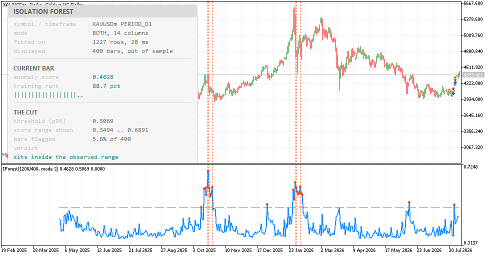
Fig. 6. The indicator on XAUUSD D1: the score curve and its dashed cut in the subwindow, the flagged bars on the price chart, and the panel confirming the cut sits inside the observed range

A gate in front of a strategy

IForest_Filter_EA.mq5 is a demonstration and claims no profit. Its entry rule is a plain Donchian breakout, chosen because it is not the point; the gate in front of it is, along with the way that gate is tested. The score has no directional content, so using it to open a position would be unreasonable, while using it to refuse one is the natural application. The EA is walk-forward by construction, refitting every N bars on bars strictly older than the bar being scored. The gate, excerpted from OnTick:

   if(InpGate != 0)
     {
      if(!g_haveModel)
        {
         g_noModel++;
         return;                      // no model yet, so no informed trade
        }
      double score = 0.0;
      if(!ScoreLastClosedBar(score))
        {
         g_noScore++;
         return;
        }
      bool anomalous = (score > g_threshold);
      bool refuse = (InpGate == 1 ? anomalous : !anomalous);
      if(refuse)
        {
         g_vetoed++;
         return;
        }
     }

Every signal that does not become a trade is counted in one of g_noModel, g_noScore, g_vetoed or g_sendFail, because a veto rate quoted against a denominator that includes bars the filter never saw is not a veto rate. The first backtest reported 3.5 percent, when 109 of its 143 signals never reached the gate at all: the Strategy Tester hands out only about 309 bars of pre-test history, and the training window asked for a thousand. Against the signals actually judged, that run gave 14.7 percent. On XAUUSD H1 from 2022 to 2026, where the window fills immediately, the gate refused 23.9 percent of the signals reaching it, five times what a calibrated percentile gives an arbitrary bar. A breakout is by construction an unusual bar, and the scan agrees independently at 23.6 percent.

Why the backtest cannot answer the question it looks like it answers

The identical strategy with the gate off, with anomalous signals skipped, and with the gate reversed produces three results that contradict each other:

Gate	Signals seen	Trades	Final balance	Per trade
Off (control)	1169	1158	25 644.81	+13.51
Skip anomalous	1342	1013	23 445.89	+13.27
Skip ordinary	2511	342	7 999.60	-5.85

Taken as totals, skipping anomalous bars hurt; taken per trade it changed almost nothing, 13.51 to 13.27; taken from the third row, anomalous bars look actively harmful. The signal counts explain why the three cannot all be right: they differ by more than a factor of two, because a strategy that trades less is flat more often and therefore observes more signals. The arms are not looking at the same sample.

The path-independent measurement lives in the scan instead. It scores every breakout bar in the untouched out-of-sample tail, whatever a strategy would have done, and splits the forward ten-bar return by the same threshold:

Breakout bars, XAUUSD H1, out-of-sample tail	count	mean forward return	win rate
Flagged anomalous	61	+6.5 bp	47.5%
Ordinary	197	+8.7 bp	53.3%

The direction is consistent with vetoing and the size is small: sixty one cases is a thin sample, the gap of 2.2 basis points is well inside what noise produces at that count, and both groups are positive. Nothing here resembles the -5.85 per trade the third backtest row implied, which is the clearest evidence that the row was path divergence.

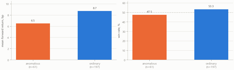
Fig. 7. The path-independent split: anomalous breakouts do marginally worse, on a sample too small to build on

The tester report fills in the rest: over 1013 trades, a profit factor of 1.19 on a 50.05 percent win rate at a 29.97 percent drawdown, with the ungated control arm finishing ahead. The equity curve rises, and none of that makes it an edge.

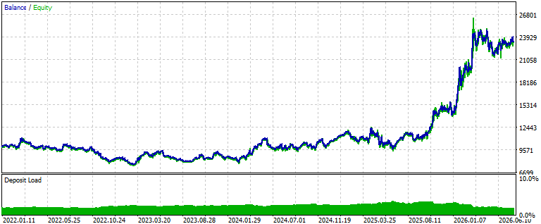
Fig. 8. The demonstration expert on XAUUSD H1 with the gate active: most of the gain arrives late in the run

Conclusion

Isolation Forest ports cleanly to MQL5 and is fast enough to be used without compromise: a hundred trees over fourteen columns grow in 2.4 milliseconds, a single bar scores in 12.4 microseconds, and a full fit over 2398 rows including calibration comes to 33. The parts that took real effort were the generator, which had to be replayable before anything could be verified, and the testing, which had to be able to come back negative.

Three results are worth carrying away. The sub-sample size is a working part of the method rather than a speed compromise, and the masking it prevents is driven by how dense an anomaly cluster is rather than how far away. Feature selection matters in an unfamiliar way, since the random column choice lets every uninformative column steal draws from the useful ones while column scale is irrelevant. And the calibrated percentile threshold transfers out of sample, which makes a live indicator and a live gate honest to build.

The limits are equally clear. The score distribution on price data is mostly explained by a null that keeps every bar's geometry and destroys only the ordering, so this detects unusual bars rather than temporal structure. The ranking is genuinely different from a z-score, but the one place it was tested against future returns produced a weak effect on a thin sample. As a detector it is a useful instrument; as an edge it would not survive a larger sample.

What was built:

• A six-header library under Include\IForest: a seedable 64-bit generator, the score functions with a percentile calibration ladder, a flat array isolation tree, the ensemble, a causal feature builder with three modes, and a facade.
• Two test scripts covering the exact arithmetic and the behavior under randomness, including a causality test that mutates a bar and demands earlier rows come back byte-identical.
• A Python cross-check that rebuilds the forest from MQL5's own numbers, and a market scan running the real series, both nulls, an out-of-sample threshold test and a forward return split in one pass.
• An indicator plotting the score curve with its calibrated cut, and a demonstration expert with a three-way anomaly gate.

#	Filename	Type	Description
1	IForest.mqh	Include	Facade: bars in, calibrated anomaly scores out
2	IForestRandom.mqh	Include	Seedable 64-bit generator and sub-sampling
3	IForestScore.mqh	Include	c(n), the anomaly score, and the percentile calibration
4	IForestTree.mqh	Include	One isolation tree over flat node arrays
5	IForestEnsemble.mqh	Include	The forest, plus per node accessors
6	IForestData.mqh	Include	Causal, scale-free feature matrix in three modes
7	IForest_Test_Core.mq5	Script	Generator conformance, c(n), score, tree contract
8	IForest_Test_Detect.mq5	Script	Planted anomaly ranking, sub-sample effect, causality
9	IForest_Scan_Market.mq5	Script	Real bars with both nulls, the baseline and the outcome split
10	IForest_Export_ForCrosscheck.mq5	Script	Dumps the bars, the features, every tree node and every score
11	IForest_Anomaly.mq5	Indicator	Score curve with its calibrated cut, marks and panel
12	IForest_Filter_EA.mq5	Expert	Demonstration of a three-way anomaly gate on a breakout
13	iforest_prototype.py	Python	Independent NumPy implementation and self-test
14	iforest_crosscheck.py	Python	Level 3: rebuilds the forest from the export and compares it node by node, then against scikit-learn
15	MQL5.zip	Archive	Archive with all project files in their subfolders; unpack it into the terminal data directory and every file lands in its required location