

Neural Networks in Trading: An End-to-End Multivariate Time Series Forecasting Model (Key Components)
 5 248
5 248
 1
1

Introduction
In the previous article, we took an in-depth look at the GinAR framework — a modern architecture for working with time series that combines the advantages of graph neural networks with the ability to train on asynchronous, incomplete, and heterogeneous data. The main idea behind this approach is to interpret a time series not as a flat sequence of observations, but as a graph structure in which individual variables or time points can be linked by arbitrary, learnable interdependencies. This approach is particularly relevant for financial modeling problems, where data are often irregular, contain missing values, and exhibit complex latent relationships.
GinAR was proposed as a versatile tool for solving such problems. Its modular structure includes several key components:
- the Interpolation Attention mechanism, which allows missing values to be reconstructed by aggregating information from observed variables;
- graph layers with individual trainable weights;
- adaptive normalization functions that make the model robust to outliers and scale instability.
The Interpolation Attention mechanism plays a central role in the architecture — it is not a classic Self-Attention kernel, but a full-fledged adaptive module capable of accounting for both global dependencies between variables and the local context of observations. In practice, this means that the model is capable, for example, of forecasting the value of a financial indicator — even in the absence of its most recent readings — by using the structure of neighboring indicators and the overall market picture. This approach is critically important in real-world conditions, where data often arrive with delays, at irregular intervals, or with significant gaps.
A key feature of GinAR is its ability to dynamically restructure the graph during training. Unlike most graph-based models, where the structure is fixed in advance, here it is formed during the training process. This makes it possible to account for changes in market conditions, correlations, and latent factors. The model independently determines which variables should be linked together, which links should be weakened, and which variables should be identified as key for the current context. This creates a flexible architecture capable of adapting to market regimes and dynamics.
Author’s visualization of the GinAR framework is shown below.
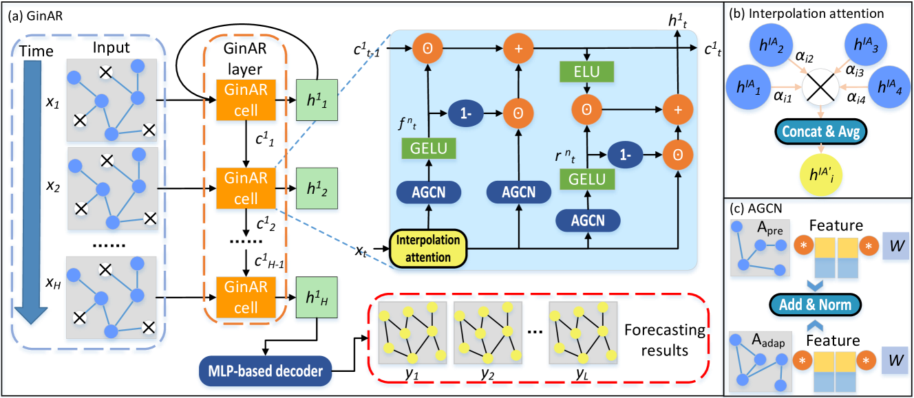
In the practical section of the previous article, we did a significant amount of work, laying the groundwork for computations within the OpenCL program. All key functions were implemented—from local reductions and computing SoftMax to the forward and backward passes in the Interpolation Attention module. Particular attention was paid to the correct handling of local memory, thread synchronization, and numerical stability, which are especially important when working with incomplete time series in a parallel computing environment.
This preparation paves the way for the next stage — integrating the model core into the main program. This is where the algorithm will come to life: data will be fed in from the trading environment, processed using OpenCL devices, run through the model, and returned as forecasts and trading decisions. This bridge between high-level logic and low-level accelerated computations is a fundamental part of our entire implementation of the GinAR architecture.
Interpolation Attention
Today we have a lot of hands-on work ahead of us related to implementing the key components of the GinAR framework. So we will not spend too much time on the theory — let's get right down to business.
The first step will be to create a key module, Interpolation Attention, which we will implement as a separate CNeuronInterpolationAttention class. This class inherits from the base object for neural layers in our library, CNeuronBaseOCL, and implements all the required logic for efficiently using the previously prepared OpenCL kernels throughout the full forward and backward pass cycle.
class CNeuronInterpolationAttention :  public CNeuronBaseOCL
  {
protected:
   //---
   uint                 iCount;
   uint                 iDimension;
   //---
   CParams              cW;
   CParams              cA;
   CParams              cGL;
   //---
   CNeuronBaseOCL       cH;
   CNeuronBaseOCL       cAdj;
   CNeuronBaseOCL       cAttention;
   //---
   virtual bool      InterpolationAttention(CNeuronBaseOCL *NeuronOCL);
   virtual bool      InterpolationAttentionGrad(CNeuronBaseOCL *NeuronOCL);
   virtual bool      feedForward(CNeuronBaseOCL *NeuronOCL) override;
   virtual bool      updateInputWeights(CNeuronBaseOCL *NeuronOCL) override;
   virtual bool      calcInputGradients(CNeuronBaseOCL *NeuronOCL) override;

public:
                     CNeuronInterpolationAttention(void) { activation = None; }
                    ~CNeuronInterpolationAttention(void) {};
   //---
   virtual bool      Init(uint numOutputs, uint myIndex, COpenCLMy *open_cl,
                          uint units_count, uint dimension,
                          ENUM_OPTIMIZATION optimization_type, uint batch);
   //---
   virtual bool      Save(const int file_handle) override;
   virtual bool      Load(const int file_handle) override;
   //---
   virtual int       Type(void) override const {  return defNeuronInterpolationAttention; }
   virtual void      TrainMode(bool flag) override;
   virtual void      SetOpenCL(COpenCLMy *obj);
   //---
   virtual bool      WeightsUpdate(CNeuronBaseOCL *source, float tau);
   virtual void      SetActivationFunction(ENUM_ACTIVATION value) override {};
  };
The class contains a set of internal variables: iCount and iDimension define the number of elements in the source data tensor, while the cW, cA, and cGL objects represent the parameters of the trainable matrices. Dedicated objects are defined separately to store intermediate results for hidden representations, the adjacency graph, and attention weights.
The core computational logic is encapsulated in the InterpolationAttention and InterpolationAttentionGrad methods, which are responsible for the model’s forward and backward passes, respectively. These methods handle the preparation and enqueuing for execution of the corresponding OpenCL kernels, which we created during the hands-on work in the previous article. These methods use an algorithm we are already familiar with, so we will not dwell on them in this article. The complete code for these methods is provided in the attachment for self-study.
All internal objects of the CNeuronInterpolationAttention class are declared as embedded member objects, which simplifies management of the instance lifecycle. Because of this, the class constructor and destructor can be left empty — they do not require explicit initialization or resource deallocation. All necessary configuration, including initialization of the class's own members and components inherited from the parent class, is performed centrally in the Init method. This provides a clean and predictable initialization structure, helping to avoid code duplication and improve reliability when the module is reused in various model configurations.
bool CNeuronInterpolationAttention::Init(uint numOutputs, uint myIndex, COpenCLMy *open_cl,
                                         uint units_count, uint dimension,
                                         ENUM_OPTIMIZATION optimization_type, uint batch)
  {
   if(!CNeuronBaseOCL::Init(numOutputs, myIndex, open_cl, units_count * dimension,
                                                        optimization_type, batch))
      return false;
In the method body, we first call the parent class's method of the same name, CNeuronBaseOCL. In this case, the layer size is recalculated taking into account the spatial dimensionality of the input signal.
Next, the model's key parameters — the number of variables and the representation dimensionality — are saved for use in calculations and internal buffer management. These parameters determine the sizes of all other vectors and matrices that will be used during the forward and backward passes.
iCount = units_count;
iDimension = dimension;
The following code block initializes the parameters and intermediate tensors used in the Interpolation Attention mechanism. First, the trainable weights cW are created; they represent an individual interaction matrix between the variables. This is a square dimension × dimension matrix.
int index = 0;
if(!cW.Init(0, index, OpenCL, iDimension * iDimension, optimization, iBatch))
   return false;
Next, the cA parameters, which are responsible for attention aggregation between nodes, are initialized.
index++;
if(!cA.Init(0, index, OpenCL, 2 * iDimension, optimization, iBatch))
   return false;
index++;
if(!cGL.Init(0, index, OpenCL, iDimension * iDimension, optimization, iBatch))
   return false;
After that, the cGL object is created, representing the latent vectors of the variables. It also has dimensions of dimension × dimension.
After all trainable parameters have been initialized, configuration of the auxiliary objects responsible for storing intermediate results begins. The cH buffer represents a matrix of linear transformations of the input signal, obtained by multiplying the input by the weights. Its dimensions are units_count × dimension.
index++;
if(!cH.Init(0, index, OpenCL, iCount * iDimension, optimization, iBatch))
   return false;
Next is the cAdj object, which stores the adjusted correlation values between the variables.
   index++;
   if(!cAdj.Init(0, index, OpenCL, iDimension * iDimension, optimization, iBatch))
      return false;
   index++;
   if(!cAttention.Init(0, index, OpenCL, iDimension * iDimension, optimization, iBatch))
      return false;
//---
   return true;
  }
Finally, cAttention is a tensor of the final attention values obtained after normalization via SoftMax.
Each initialization is followed by a check to verify that it was successful. If a failure occurs at any stage, the method immediately returns false, providing reliable protection against configuration errors.
If all objects have been successfully configured and placed in the memory of the OpenCL device, the method completes, returning true. This means that the layer is fully ready to run and can be used as part of the model.
Once the object initialization is complete, we move on to setting up the forward pass process, which we implement in the feedForward method. Its task is to properly prepare all the input data and run the main computation using the OpenCL kernel developed earlier. The algorithm is fairly compact, but it includes several key stages, each of which plays an important role in the layer's overall operation.
bool CNeuronInterpolationAttention::feedForward(CNeuronBaseOCL *NeuronOCL)
  {
   if(bTrain)
     {
      if(!cW.FeedForward())
         return false;
      if(!cA.FeedForward())
         return false;
      if(!cGL.FeedForward())
         return false;
     }
   if(!InterpolationAttention(NeuronOCL))
      return false;
//---
   return true;
  }
First, the method checks whether the bTrain flag is set, which indicates that the layer is in training mode. This is critical because, in this case, the model's trainable parameters must first be run through their own FeedForward methods. This call is necessary to update their values and ensure their participation in the current computation cycle. All three calls include a success check, and at the slightest failure, the method immediately stops executing and returns false. This prevents a situation in which uninitialized or invalid parameters are carried forward into subsequent calculations.
Once all preparatory steps are complete, the main InterpolationAttention method is called. This function initiates the launch of the OpenCL kernel responsible for computing attention, aggregating values, and generating the layer's output representation.
The method completes its execution by returning the Boolean result of the operations to the caller.
The calcInputGradients method is implemented in an extremely concise manner, since all of the backpropagation logic has already been moved into the corresponding OpenCL kernel. Here, we simply call the wrapper function InterpolationAttentionGrad, which is responsible for launching the kernel and passing the necessary buffers. Then we return the Boolean result of the operations to the caller.
bool CNeuronInterpolationAttention::calcInputGradients(CNeuronBaseOCL *NeuronOCL)
  {
   if(!InterpolationAttentionGrad(NeuronOCL))
      return false;
//---
   return true;
  }
This implementation fully preserves the overall operating structure of neural layers, allowing this module to be used alongside other types of layers without any changes to the training logic. This highlights the system's architectural flexibility and makes integrating new solutions as simple and safe as possible.
The update of trainable parameters in the module is implemented as compactly and logically as possible. All weights used in the calculations are internal objects of the class (cW, cA, cGL), each of which encapsulates its own update algorithm. The updateInputWeights method simply invokes the corresponding functions on them, ensuring modularity and a clean architecture.
bool CNeuronInterpolationAttention::updateInputWeights(CNeuronBaseOCL *NeuronOCL)
  {
   if(!cW.UpdateInputWeights())
      return false;
   if(!cA.UpdateInputWeights())
      return false;
   if(!cGL.UpdateInputWeights() ||
      !Normilize(cGL.getWeightsParams(), 2 * iDimension))
      return false;
//---
   return true;
  }
Special attention is given to the cGL tensor, which, after being updated, is additionally normalized using the Normilize function. This is necessary because cGL contains the weights of the correlation-based links between variables, and the stability of these coefficients directly affects the stability of the entire attention module. Normalization helps smooth out any outliers and preserve the interpretability of the weights. Thus, this method fully completes the training cycle without requiring any additional intervention or configuration.
The complete source code for the CNeuronInterpolationAttention class, along with the implementation of all its methods, can be found in the attachment. We have deliberately avoided overloading this article with technical details to keep the text lively; however, we recommend reviewing the source code to fully understand the module’s logic and how it integrates into the overall GinAR framework.
AGCN
The next logical step in developing the GinAR framework is to implement the adaptive graph convolution (AGCN) mechanism. This is a key component of the framework that makes it possible to account for complex relationships between time series represented as nodes in a graph. Unlike traditional approaches, in which the graph structure is specified in advance and remains fixed throughout training, adaptive convolution allows the model to independently form and modify the topology of connections based on the current state of the data. This flexibility is critical when working with dynamic financial time series, whose structure is subject to constant fluctuations, hidden interrelationships, and external disturbances.
To implement this idea, a separate module was developed as the CNeuronAGCN class. This class inherits from the base fully connected layer, CNeuronBaseOCL, and encapsulates all the logic required to perform adaptive convolution using OpenCL acceleration. Its internal structure is designed to ensure maximum computational efficiency and accuracy at every stage of processing, including feature extraction, connection matrix formation, normalization, aggregation, and training the graph weights.
A distinctive feature of this module is that, during information processing, it does not rely on a fixed adjacency matrix but computes it in real time. To this end, the input data passes through a sequence of transformations, resulting in a latent representation for each node. These representations are used to compute the similarity between nodes, on the basis of which the matrix of adaptive connections is constructed. In this way, the model essentially looks at each time series and decides on its own which other series to connect it to — and with what strength. The result is a flexible attention mechanism in which each node is capable of adapting its behavior based on the context.
The structure of the new class is shown below.
class CNeuronAGCN    :  public CNeuronBaseOCL
  {
protected:
   CParams              cEa;
   CNeuronSwiGLUOCL     cWx;
   CNeuronSwiGLUOCL     cWe;
   CNeuronBaseOCL       cWconcat_ex;
   CNeuronConvOCL       cEn;
   CNeuronTransposeOCL  cEnT;
   CNeuronBaseOCL       cEnEnT;
   CNeuronSoftMaxOCL    cAadapt;
   CNeuronBaseOCL       cAadaptX;
   CNeuronBaseOCL       cApreX;
   CNeuronSwiGLUOCL     cWadapt;
   CNeuronSwiGLUOCL     cWpre;
   //---
   virtual bool      feedForward(CNeuronBaseOCL *NeuronOCL) override { return false; }
   virtual bool      feedForward(CNeuronBaseOCL *NeuronOCL, CBufferFloat *SecondInput) override;
   virtual bool      updateInputWeights(CNeuronBaseOCL *NeuronOCL) override { return false; }
   virtual bool      updateInputWeights(CNeuronBaseOCL *NeuronOCL, CBufferFloat *second) override;
   virtual bool      calcInputGradients(CNeuronBaseOCL *NeuronOCL) override { return false; }
   virtual bool      calcInputGradients(CNeuronBaseOCL *NeuronOCL,
                                        CBufferFloat *SecondInput,
                                        CBufferFloat *SecondGradient,
                                        ENUM_ACTIVATION SecondActivation = None) override;

public:
                     CNeuronAGCN(void) {activation = None;}
                    ~CNeuronAGCN(void) {};
   //---
   virtual bool      Init(uint numOutputs, uint myIndex, COpenCLMy *open_cl,
                          uint units_count, uint dimension,
                          ENUM_OPTIMIZATION optimization_type, uint batch);
   //---
   virtual bool      Save(const int file_handle) override;
   virtual bool      Load(const int file_handle) override;
   //---
   virtual int       Type(void) override const  {  return defNeuronAGCN; }
   virtual void      TrainMode(bool flag) override;
   virtual void      SetOpenCL(COpenCLMy *obj);
   //---
   virtual bool      WeightsUpdate(CNeuronBaseOCL *source, float tau);
   //---
   virtual uint      GetWindow(void) const      { return cWx.GetWindow(); }
   virtual uint      GetUnits(void) const       { return cWx.GetUnits(); }
   virtual void      SetActivationFunction(ENUM_ACTIVATION value) override {};
  };
The entire computational chain is organized within a single object, but it includes many auxiliary layers and operations. The logic is broken down into stages, which we will explore as we implement the class methods. The output features can be interpreted as the result of coordinated filtering over an adapted graph, taking into account both content information and topological relationships between the time series.
As with the previous layer, all internal components of the CNeuronAGCN class were declared statically. This approach allows us to leave the class constructor and destructor empty, concentrating all the initialization logic in a single method: Init. This ensures a compact implementation and also makes it easier to manage the lifecycle of objects within the layer.
bool CNeuronAGCN::Init(uint numOutputs, uint myIndex, COpenCLMy *open_cl,
                       uint units_count, uint dimension,
                       ENUM_OPTIMIZATION optimization_type, uint batch)
  {
   if(!CNeuronBaseOCL::Init(numOutputs, myIndex, open_cl,
                            units_count * dimension, optimization_type, batch))
      return false;
Initialization begins with a call to the method of the same name in the parent class, where the initial configuration of the interfaces and general layer parameters is performed. After that, all the key components of the adaptive graph convolution are configured step by step.
In the first step, a cEa object is created, which will be used to encode additional information about the data structure.
//---
   int index = 0;
   if(!cEa.Init(0, index, OpenCL, Neurons(), optimization, iBatch))
      return false;
   cEa.SetActivationFunction(None);
Next, two important layers — cWx and cWe — are initialized; they are responsible for extracting features from the input data and the previously learned structure of the time series. Both layers are implemented using the SwiGLU mechanism and are trained in parallel.
index++;
if(!cWx.Init(0, index, OpenCL, dimension, dimension, dimension, units_count,
                                                   1, optimization, iBatch))
   return false;
index++;
if(!cWe.Init(0, index, OpenCL, dimension, dimension, dimension, units_count,
                                                   1, optimization, iBatch))
   return false;
These are followed by the cWconcat_ex buffer, which combines representations in latent space.
index++;
if(!cWconcat_ex.Init(0, index, OpenCL, 2 * Neurons(), optimization, iBatch))
   return false;
cWconcat_ex.SetActivationFunction(None);
The next element in the initialization process is the cEn layer, which performs a linear transformation of the combined features. It is supplemented by the cEnT transposition module, which prepares the data for forming a preliminary attention matrix.
index++;
if(!cEn.Init(0, index, OpenCL, 2 * dimension, 2 * dimension, dimension, units_count,
                                                           1, optimization, iBatch))
   return false;
cEn.SetActivationFunction(None);
index++;
if(!cEnT.Init(0, index, OpenCL, units_count, dimension, optimization, iBatch))
   return false;
index++;
if(!cEnEnT.Init(0, index, OpenCL, units_count * units_count, optimization, iBatch))
   return false;
cEnEnT.SetActivationFunction(GELU);
After the transposition step, the prepared data are passed to the matrix multiplication operation, where a dot-product operation is performed between the original representation and its transposed version. The result is a symmetric relationship matrix, which is stored in the cEnEnT object. It is in this block that the resulting values are passed through the GELU function; this function allows negative correlations to be gently suppressed without completely eliminating them, while also reducing their contribution to the final representation.
This approach helps identify the most significant patterns and latent relationships between the nodes of the graph, which is critically important when constructing an adaptive attention matrix. Ultimately, thanks to this operation, the model is able to capture deeper structural patterns within the graph and correctly weigh inter-node interactions.
Next comes a key step — normalizing the obtained values. For this, the SoftMax function is used, which is applied inside the cAadapt object. This operation converts raw weight coefficients into a probability distribution, in which each edge between graph nodes is assigned a specific degree of significance. Thus, weak and noisy dependencies are suppressed, while strong and informative ones are amplified. The result is a fully formed adaptive attention matrix that reflects the individual interaction patterns among the components of the input signal.
index++;
if(!cAadapt.Init(0, index, OpenCL, units_count * units_count, optimization, iBatch))
   return false;
cAadapt.SetHeads(units_count);
The next logical operation is to apply the adaptive weights to the input data. This stage is carried out by weighting the input features with the corresponding attention coefficients. The result is stored in the cAadaptX buffer, which represents an updated, context-enriched representation of the input signal. Essentially, this is a reweighted projection of the original input that takes into account the identified relationships between individual nodes in the graph.
index++;
if(!cAadaptX.Init(0, index, OpenCL, Neurons(), optimization, iBatch))
   return false;
cAadaptX.SetActivationFunction(None);
index++;
if(!cApreX.Init(0, index, OpenCL, Neurons(), optimization, iBatch))
   return false;
cApreX.SetActivationFunction(None);
An additional processing step involves adapting the input data with regard to a predefined graph structure. This step is intended to amplify the influence of known, a priori relationships between nodes that were derived outside the model being trained — for example, based on fundamental relationships, topology, or expert rules. The mechanism here is similar to the previous one: weights are applied to the original tensor, but not from the adaptive attention matrix; instead, they come from an external coefficient matrix. The result is stored in the cApreX buffer. Thus, the model receives two independent information channels at once — one based on automatic learning and identified patterns, and the other on structural a priori information. Combining them makes it possible to achieve a better balance between the model's flexibility and robustness.
Finally, in the final part of the initialization process, two convolutional layers are created: cWadapt and cWpre. Both use the SwiGLU architecture, acting as filters that adapt the features to the structure of the generated connection matrix.
   index++;
   if(!cWadapt.Init(0, index, OpenCL, dimension, dimension, dimension, units_count,
                                                          1, optimization, iBatch))
      return false;
   cWadapt.SetActivationFunction(None);
   index++;
   if(!cWpre.Init(0, index, OpenCL, dimension, dimension, dimension, units_count, 1,
                                                              optimization, iBatch))
      return false;
   cWpre.SetActivationFunction(None);
   SetActivationFunction(None);
//---
   return true;
  }
Once all these steps are complete, we explicitly disable the layer's activation function, since the nonlinearities are applied within the internal blocks and there is no need to duplicate them at the output.
Thus, the entire Init method is a carefully organized sequence of steps during which all elements of the adaptive convolution are created and configured. Each component is responsible for a specific part of the computations and fits into the overall architecture of the layer, forming the foundation for the model's further operation.
The next stage of our work is the feedForward method, which implements the full forward pass cycle of adaptive graph convolution, taking into account both trainable and externally specified structural connections. The algorithm is quite involved, so let's examine it step by step, focusing on the semantic logic of each block.
bool CNeuronAGCN::feedForward(CNeuronBaseOCL *NeuronOCL, CBufferFloat *SecondInput)
  {
   if(!SecondInput || SecondInput.Total() < cAadapt.Neurons())
      return false;
Before the algorithm begins executing, a mandatory check is performed to verify the validity of the input data: if the matrix of predefined correlation coefficients, SecondInput, is missing, or if its size is insufficient to perform matrix operations, execution is immediately terminated.
Next, if the model is in training mode, the parameter preparation loop is started for the branch responsible for the adaptive context of the nodes. First, a forward pass is performed through the cEa object, which contains the trainable parameters for computing edge embeddings. The result is passed to cWe, where the matrix of external interaction weights is formed, with the weights reflecting the context of the connections between nodes at the current training step.
if(bTrain)
  {
   if(!cEa.FeedForward())
      return false;
   if(!cWe.FeedForward(cEa.AsObject()))
      return false;
  }
At the same time, the main branch — the one that works with the primary sequence of features — is activated. In this branch, the cWx forward pass method is called, forming a representation of the current state of the nodes.
if(!cWx.FeedForward(NeuronOCL))
   return false;
if(!Concat(cWx.getOutput(), cWe.getOutput(), cWconcat_ex.getOutput(),
             cWx.GetWindowOut(), cWe.GetWindowOut(), cWx.GetUnits()))
   return false;
After that, the two output vectors (cWx and cWe) are concatenated across individual sequence elements, which allows the model to take structural and contextual information into account in subsequent operations. The resulting output is used in cEn, which performs a linear convolution that reduces dimensionality and enhances meaningful features.
if(!cEn.FeedForward(cWconcat_ex.AsObject()))
   return false;
if(!cEnT.FeedForward(cEn.AsObject()))
   return false;
if(!MatMul(cEn.getOutput(), cEnT.getOutput(), cEnEnT.getOutput(),
             cEnT.GetCount(), cEnT.GetWindow(), cEnT.GetCount()))
   return false;
if(cEnEnT.Activation() != None)
   if(!Activation(cEnEnT.getOutput(), cEnEnT.getOutput(), cEnEnT.Activation()))
      return false;
Next, a key operation takes place: transposing the resulting matrix and multiplying it by the original matrix, which allows a symmetric correlation matrix to be constructed in the cEnEnT object. If an activation function (in our case, GELU) is applied to this object, it is invoked, thereby mitigating the effects of noise and negative correlations.
The resulting matrix is then passed to the cAadapt object, where the SoftMax mechanism is applied within a multi-head attention structure. It normalizes the weights row-wise and returns an attention matrix adapted to the current data structure. To strengthen the diagonal connections, the IdentSum function is called; it adds an identity matrix to the result, which ensures the graph's robustness to sparse inputs.
if(!cAadapt.FeedForward(cEnEnT.AsObject()))
   return false;
if(!IdentSum(cAadapt.getOutput(), cAadapt.getOutput(), cAadapt.Heads()))
   return false;
The model then computes two parallel matrix multiplication streams. The first stream works with the external data SecondInput, multiplying it by the current outputs of the neural layer; the result is stored in the cApreX buffer. The second stream works similarly with the cAadapt attention matrix and the current outputs, storing the result in cAadaptX.
if(!MatMul(SecondInput, NeuronOCL.getOutput(), cApreX.getOutput(),
           cWpre.GetUnits(), cWpre.GetUnits(), cWpre.GetWindow()))
   return false;
if(!MatMul(cAadapt.getOutput(), NeuronOCL.getOutput(), cAadaptX.getOutput(),
           cWadapt.GetUnits(), cWadapt.GetUnits(), cWadapt.GetWindow()))
   return false;
The final step is to pass both streams through the trainable convolutional blocks cWpre and cWadapt. This allows the model to refine the resulting data with respect to local features.
   if(!cWpre.FeedForward(cApreX.AsObject()))
      return false;
   if(!cWadapt.FeedForward(cAadaptX.AsObject()))
      return false;
   if(!SumAndNormilize(cWadapt.getOutput(), cWpre.getOutput(), Output, cWadapt.GetWindowOut(), true))
      return false;
//---
   return true;
  }
After that, the SumAndNormilize function is called; it combines both streams and brings the result into the required form at the layer output.
Thus, the method implements several powerful mechanisms at once: adaptive attention, feature extraction, structural integration, and convolutional transformation. All of this turns the module into a full-fledged graph processing block capable of taking into account both internal dependencies between nodes and external structural constraints.
Once the forward pass in adaptive graph convolution (AGCN) is complete, one of the most critical stages begins: propagating error gradients from the layer output to its trainable components. As part of this process, backpropagation is performed, making it possible to precisely determine each object’s contribution to the final result and adjust the parameters to minimize the error. The entire algorithm is implemented within the calcInputGradients method.
bool CNeuronAGCN::calcInputGradients(CNeuronBaseOCL *NeuronOCL,
                                     CBufferFloat *SecondInput,
                                     CBufferFloat *SecondGradient,
                                     ENUM_ACTIVATION SecondActivation = -1)
  {
   if(!NeuronOCL || !SecondInput || !SecondGradient ||
      SecondInput.Total() < cAadapt.Neurons() ||
      SecondGradient.Total() < cAadapt.Neurons())
      return false;
In the first step, a standard validation check of the input data is performed: if the received pointers are not initialized, or if the input buffers are not large enough to perform matrix operations, execution of the method stops. Next, the actual error distribution begins.
Backpropagation in the AGCN block starts from the very end — specifically, from the layer output, where the final result has already been formed. In our case, this is the sum of the outputs of two key components: cWadapt and cWpre. As a reminder, it is these components that contribute to building the final representation, which generalizes both attention and the static structure of the graph.
Since the block output is a simple sum of two tensors, the error gradient received from the subsequent layer must be passed equally to both modules — without any additional weighting coefficients. However, before we begin calculating gradients through the internal connections of each module, we must adjust this gradient to account for the activation functions used in the forward pass. To do this, the DeActivation method is called — essentially, it multiplies the obtained gradient by the derivative of the activation function applied to the outputs of cWadapt and cWpre. This is a crucial step; without it, backpropagation through nonlinear transformations would be incorrect.
if(!DeActivation(cWadapt.getOutput(), cWadapt.getGradient(), Gradient, cWadapt.Activation()))
   return false;
if(!DeActivation(cWpre.getOutput(), cWpre.getGradient(), Gradient, cWpre.Activation()))
   return false;
After that, the error is distributed to their inputs: the CalcHiddenGradients methods are called for the cAadaptX and cApreX objects, through which the streams passed that were formed using the matrices of adaptive and predefined connections between nodes, respectively.
if(!cApreX.CalcHiddenGradients(cWpre.AsObject()))
   return false;
if(!cAadaptX.CalcHiddenGradients(cWadapt.AsObject()))
   return false;
Next, using MatMulGrad, backpropagation is performed through the multiplication operation: the contribution of each component to the total error is computed. If an activation function is used, its reverse transformation is performed using DeActivation, which allows the true error to be restored to its pre-normalization state.
   if(!MatMulGrad(SecondInput, SecondGradient,
                  NeuronOCL.getOutput(), NeuronOCL.getGradient(),
                  cApreX.getGradient(), cWpre.GetUnits(),
                  cWpre.GetUnits(), cWpre.GetWindow()))
      return false;
   if(SecondActivation != None)
      if(!DeActivation(SecondInput, SecondGradient,
                       SecondGradient, SecondActivation))
         return false;
//---
   if(!MatMulGrad(cAadapt.getOutput(), cAadapt.getGradient(),
                  NeuronOCL.getOutput(), PrevOutput,
                  cAadaptX.getGradient(),  cWadapt.GetUnits(),
                  cWadapt.GetUnits(), cWadapt.GetWindow()))
      return false;
   if(!SumAndNormilize(NeuronOCL.getGradient(), PrevOutput,
                       PrevOutput, cWx.GetWindow(), false))
      return false;
   if(NeuronOCL.Activation() != None)
      if(!DeActivation(NeuronOCL.getOutput(), PrevOutput,
                       PrevOutput, NeuronOCL.Activation()))
         return false;
Please note that in both matrix multiplication operations performed during the forward pass, the input data from the main information stream was used. Therefore, we need to accumulate the error gradient along both branches. We use the temporary buffer PrevOutput to accumulate the values. If NeuronOCL uses an activation function, its derivative is applied to correctly recalculate the gradient, taking nonlinearity into account.
The next key step is backpropagation through the cEnEnT correlation matrix, which was obtained earlier during the forward pass. First, the hidden gradients are computed; then, if the GELU function was used, deactivation is applied at the output.
if(!cEnEnT.CalcHiddenGradients(cAadapt.AsObject()))
   return false;
if(cEnEnT.Activation() != None)
   if(!DeActivation(cEnEnT.getOutput(), cEnEnT.getGradient(),
                    cEnEnT.getGradient(), cEnEnT.Activation()))
      return false;
Next, MatMulGrad is called, implementing backward gradient propagation through the operation of multiplying the features by their transposed copy.
if(!MatMulGrad(cEn.getOutput(), cEn.getPrevOutput(),
               cEnT.getOutput(), cEnT.getGradient(),
               cEnEnT.getGradient(), cEnT.GetCount(),
               cEnT.GetWindow(), cEnT.GetCount()))
   return false;
Additionally, transposed errors are passed to the cEn layer, where they are summed with previously obtained values, and deactivation is performed if an activation function was used.
if(!cEn.CalcHiddenGradients(cEnT.AsObject()))
   return false;
if(!SumAndNormilize(cEn.getGradient(), cEn.getPrevOutput(),
                    cEn.getGradient(), cEnT.GetWindow(), false))
   return false;
if(cEn.Activation() != None)
   if(!DeActivation(cEn.getOutput(), cEn.getGradient(),
                    cEn.getGradient(), cEn.Activation()))
      return false;
Immediately afterward, the gradients are fed into cWconcat_ex, where the reverse process of separating the features begins (recall that they were combined during the forward pass).
if(!cWconcat_ex.CalcHiddenGradients(cEn.AsObject()))
   return false;
if(!DeConcat(cWx.getGradient(), cWe.getGradient(), cWconcat_ex.getGradient(),
             cWx.GetWindowOut(), cWe.GetWindowOut(), cWx.GetUnits()))
   return false;
if(cWx.Activation() != None)
   if(!DeActivation(cWx.getOutput(), cWx.getGradient(),
                    cWx.getGradient(), cWx.Activation()))
      return false;
if(cWe.Activation() != None)
   if(!DeActivation(cWe.getOutput(), cWe.getGradient(),
                    cWe.getGradient(), cWe.Activation()))
      return false;
The DeConcat function correctly splits the gradients into two parts — one for cWx and one for cWe. In each of these modules, DeActivation is called separately, restoring the clean gradient. Next, backpropagation proceeds through the network: first to the input data level via `cWx`, then to cEa via cWe.
   if(!NeuronOCL.CalcHiddenGradients(cWx.AsObject()))
      return false;
   if(!SumAndNormilize(NeuronOCL.getGradient(), PrevOutput,
                       NeuronOCL.getGradient(), cWx.GetWindow(), false))
      return false;
   if(!cEa.CalcHiddenGradients(cWe.AsObject()))
      return false;
//---
   return true;
  }
Note that we have already passed the error gradient to the input data level of the main branch, so we sum the resulting values with those accumulated earlier.
It is worth noting in particular that the method implements a strict sequence of all steps. This is necessary because the error must be propagated backward strictly in the reverse order of the forward pass. Each step carefully compensates for the effects of convolutions, normalizations, activations, and transpositions. Only at the end, after the gradients have been fully computed, is the model ready to update its weights, maintaining accuracy at every stage of training.
The method for updating parameters is implemented in an extremely straightforward, yet elegant and reliable way. There are no complex conditions or additional calculations here — it all comes down to carefully passing control to internal objects that directly contain the trainable weights. Each of them implements its own update mechanism based on accumulated gradients and the selected optimization scheme.
bool CNeuronAGCN::updateInputWeights(CNeuronBaseOCL *NeuronOCL, CBufferFloat *second)
  {
   if(!cEa.UpdateInputWeights())
      return false;
   if(!cWe.UpdateInputWeights(cEa.AsObject()))
      return false;
   if(!cWx.UpdateInputWeights(NeuronOCL))
      return false;
   if(!cEn.UpdateInputWeights(cWconcat_ex.AsObject()))
      return false;
   if(!cWpre.UpdateInputWeights(cApreX.AsObject()))
      return false;
   if(!cWadapt.UpdateInputWeights(cAadaptX.AsObject()))
      return false;
//---
   return true;
  }
Each method is called with the appropriate input object obtained during the forward pass, which preserves computational correctness under the graph topology.
This approach makes the code structure not only readable but also easily scalable.
For the reader's convenience and to ensure complete technical transparency, the entire source code for this class, including the definitions of all methods, is provided in the attachment.
GinAR Cell
We now move on to the final stage — the creation of a full-fledged GinAR computational cell, which integrates all the components discussed earlier into a single, cohesive structure. It is here, in the CNeuronGinARCell class, that the mechanisms of Interpolation Attention, adaptive graph convolution, and memory control elements converge to form a flexible yet strictly structured architecture.
class CNeuronGinARCell  :  public CNeuronBaseOCL
  {
protected:
   CNeuronInterpolationAttention cX_IA;
   CNeuronAGCN                   cX_AGCN;
   CNeuronAGCN                   cForgetGate;
   CNeuronAGCN                   cResetGate;
   CNeuronBaseOCL                cContext;
   CBufferFloat                  bTemp;
   //---
   virtual bool      feedForward(CNeuronBaseOCL *NeuronOCL) override { return false; }
   virtual bool      feedForward(CNeuronBaseOCL *NeuronOCL, CBufferFloat *SecondInput) override;
   virtual bool      updateInputWeights(CNeuronBaseOCL *NeuronOCL) override { return false; }
   virtual bool      updateInputWeights(CNeuronBaseOCL *NeuronOCL, CBufferFloat *second) override;
   virtual bool      calcInputGradients(CNeuronBaseOCL *NeuronOCL) override { return false; }
   virtual bool      calcInputGradients(CNeuronBaseOCL *NeuronOCL,
                                        CBufferFloat *SecondInput,
                                        CBufferFloat *SecondGradient,
                                        ENUM_ACTIVATION SecondActivation = None) override;

public:
                     CNeuronGinARCell(void) { activation = None;}
                    ~CNeuronGinARCell(void) {};
   //---
   virtual bool      Init(uint numOutputs, uint myIndex, COpenCLMy *open_cl,
                          uint units_count, uint dimension,
                          ENUM_OPTIMIZATION optimization_type, uint batch);
   //---
   virtual bool      Save(const int file_handle) override;
   virtual bool      Load(const int file_handle) override;
   //---
   virtual int       Type(void) override const  {  return defNeuronGinARCell; }
   virtual void      TrainMode(bool flag) override;
   virtual void      SetOpenCL(COpenCLMy *obj);
   //---
   virtual bool      WeightsUpdate(CNeuronBaseOCL *source, float tau);
   virtual void      SetActivationFunction(ENUM_ACTIVATION value) override {};
  };
In the structure of the new object shown above, it is clear that CNeuronGinARCell inherits the base interface from CNeuronBaseOCL. This ensures compatibility with the framework's other layers and modules. However, unlike simple blocks, this one combines several functional components:
- cX_IA — an Interpolation Attention block responsible for smoothing and adjusting the input time series;
- cX_AGCN — the main adaptive graph convolution module, which forms a generalized representation of the input features while taking their relationships into account;
- cForgetGate and cResetGate are two additional graph-based subsystems that implement forget and reset mechanisms similar to those in GRU cells;
- cContext — an internal buffer that stores the accumulated state of the hidden memory;
- bTemp — a temporary buffer used in intermediate computations.
The class implements the standard execution cycle of a neural layer. The Init method initializes all components of CNeuronGinARCell step by step. This is where the model's main parameters are specified: the number of outputs, the feature space dimensionality, the optimization type, and the batch size.
bool CNeuronGinARCell::Init(uint numOutputs, uint myIndex, COpenCLMy *open_cl,
                            uint units_count, uint dimension,
                            ENUM_OPTIMIZATION optimization_type, uint batch)
  {
   if(!CNeuronBaseOCL::Init(numOutputs, myIndex, open_cl,
                            units_count * dimension, optimization_type, batch))
      return false;
Next, the cell's internal blocks are initialized one by one. First, cX_IA, which is responsible for Interpolation Attention, is initialized.
int index = 0;
if(!cX_IA.Init(0, index, OpenCL, units_count, dimension, optimization, iBatch))
   return false;
Next, the main graph convolution module, cX_AGCN, is initialized, followed by the control gates cForgetGate and cResetGate. Each one is assigned its own unique index.
index++;
if(!cX_AGCN.Init(0, index, OpenCL, units_count, dimension, optimization, iBatch))
   return false;
index++;
if(!cForgetGate.Init(0, index, OpenCL, units_count, dimension, optimization, iBatch))
   return false;
index++;
if(!cResetGate.Init(0, index, OpenCL, units_count, dimension, optimization, iBatch))
   return false;
As a separate step, the cContext module is initialized, serving as an accumulator for the internal state. Its output is explicitly filled with zeros to avoid random noise at startup, and the activation function is disabled, allowing it to be used as a pure storage buffer.
   index++;
   if(!cContext.Init(0, index, OpenCL, units_count * dimension, optimization, iBatch))
      return false;
   if(!cContext.getPrevOutput().Fill(0))
      return false;
   cContext.SetActivationFunction(None);
   bTemp.BufferFree();
   if(!bTemp.BufferInit(units_count * units_count, 0) ||
      !bTemp.BufferCreate(OpenCL))
      return false;
//---
   return true;
  }
Finally, a temporary buffer, bTemp, is created to perform intermediate operations. The buffer size is chosen to be quadratic: units_count * units_count. In this case, if the buffer has already been created, it is freed first, which ensures correct operation and conserves resources.
After completing all operations, the method then returns a Boolean result to the caller.
The forward pass algorithm built in the feedForward method implements the key operating logic of CNeuronGinARCell, combining attention mechanisms, graph convolutions, and memory management through the forget gate and reset gate.
bool CNeuronGinARCell::feedForward(CNeuronBaseOCL *NeuronOCL, CBufferFloat *SecondInput)
  {
   if(!cX_IA.FeedForward(NeuronOCL))
      return false;
In the first stage, the cX_IA module is activated, performing an interpolation transformation on the source data from NeuronOCL. The resulting representation is used as the basis for three parallel blocks — the main graph convolutional module cX_AGCN, as well as the cForgetGate and cResetGate modules, which are responsible for generating control masks.
if(!cX_AGCN.FeedForward(cX_IA.AsObject(), SecondInput))
   return false;
if(!cForgetGate.FeedForward(cX_IA.AsObject(), SecondInput))
   return false;
if(!cResetGate.FeedForward(cX_IA.AsObject(), SecondInput))
   return false;
if(!Activation(cForgetGate.getOutput(), cForgetGate.getOutput(), GELU))
   return false;
if(!Activation(cResetGate.getOutput(), cResetGate.getOutput(), GELU))
   return false;
Each of these three blocks also accepts a second input, SecondInput, which contains graph or structural information — an adjacency matrix or data about neighboring nodes. After passing through the layers, the outputs of the cForgetGate and cResetGate gates are passed through the GELU activation function, allowing smoother, more flexible masks to be created that reduce the impact of abrupt transitions and negative values.
Next, the internal context is updated. It is worth noting here that during the forward pass, the context values needed for backward pass operations are immediately overwritten. To prevent this, we use a buffer carousel: we call the SwapOutputs method, which swaps the buffer pointers Output and PrevOutput.
//--- Context
   if(!cContext.SwapOutputs())
      return false;
   if(!GateElementMult(cContext.getPrevOutput(), cX_AGCN.getOutput(),
                       cForgetGate.getOutput(), cContext.getOutput()))
      return false;
Next, a new context vector is formed through element-wise multiplication of the previous state of cContext and the results of cX_AGCN, weighted by the forget mask cForgetGate. This allows flexible control over which memory elements should be preserved and which should be zeroed out.
The new context vector passes through an ELU activation function adapted to handle negative values, which improves gradient stability.
//--- Output
   if(!Activation(cContext.getOutput(), cContext.getPrevOutput(), ELU))
      return false;
   if(!GateElementMult(cContext.getPrevOutput(), cX_IA.getOutput(), cResetGate.getOutput(), Output))
      return false;
//---
   return true;
  }
Finally, the block's final output in the Output buffer is formed by element-wise multiplication of the updated context, the result tensor cX_IA, and the mask cResetGate. This step combines the long-term memory, the current input state, and the reset mask, which is responsible for passing relevant features to the output.
If an error or failure occurs at any stage while performing the operation, the method returns false. If all operations are completed successfully, it returns true, confirming that the data has passed correctly through the entire cell structure.
The backpropagation algorithm is not as simple as it might seem at first glance. Its main complexity lies in the need to carefully sum and normalize gradients from multiple sources, since the input data from both branches is used in several places at once: in the main stream (cX_AGCN) and in auxiliary paths through the control gates cForgetGate and cResetGate. Therefore, each of these consumers generates its own contribution to the final gradient, and all of them must be correctly combined.
bool CNeuronGinARCell::calcInputGradients(CNeuronBaseOCL *NeuronOCL,
                                          CBufferFloat *SecondInput,
                                          CBufferFloat *SecondGradient,
                                          ENUM_ACTIVATION SecondActivation = -1)
  {
   if(!NeuronOCL || !SecondInput || !SecondGradient)
      return false;
//--- Output
   if(!GateElementMultGrad(cContext.getPrevOutput(), cContext.getGradient(),
                           cX_IA.getOutput(), cX_IA.getPrevOutput(),
                           cResetGate.getOutput(), cResetGate.getGradient(),
                           Gradient, ELU, cX_IA.Activation(), GELU))
      return false;
First, the gradient of the cell's final output is distributed among the context cContext, the Interpolation Attention result cX_IA, and the reset gate cResetGate. In this process, all derivatives with respect to the corresponding activation functions are taken into account.
Next, the gradient of the internal memory state cContext is reconstructed. Since it is formed from the results of multiplying the output of the main convolutional module cX_AGCN by the cForgetGate mask, a similar backpropagation operation is used. Other activation functions and other gradients are involved here, and the result is accumulated in the cContext object.
//--- Context
   if(!GateElementMultGrad(cContext.getOutput(), cContext.getPrevOutput(),
                           cX_AGCN.getOutput(), cX_AGCN.getGradient(),
                           cForgetGate.getOutput(), cForgetGate.getGradient(),
                           cContext.getGradient(), None,
                           cX_AGCN.Activation(), GELU))
      return false;
Next comes one of the most critical steps — passing the gradients back to the cX_IA Interpolation Attention module. It served as the common predecessor of the three branches, so three independent calls to CalcHiddenGradients are required, one for each path: the main branch (cX_AGCN), the forget gate (cForgetGate), and the reset gate (cResetGate).
//--- Gradient to Interpolation Attention
   if(!cX_IA.CalcHiddenGradients(cX_AGCN.AsObject(), SecondInput,
                                 SecondGradient, SecondActivation) ||
      !SumAndNormilize(cX_IA.getGradient(), cX_IA.getPrevOutput(),
                       cX_IA.getPrevOutput(), cForgetGate.GetWindow(), false, 0, 0, 0, 1))
      return false;
   if(!cX_IA.CalcHiddenGradients(cForgetGate.AsObject(), SecondInput,
                                 GetPointer(bTemp), SecondActivation) ||
      !SumAndNormilize(cX_IA.getGradient(), cX_IA.getPrevOutput(),
                       cX_IA.getPrevOutput(), cForgetGate.GetWindow(), false, 0, 0, 0, 1) ||
      !SumAndNormilize(SecondGradient, GetPointer(bTemp),
                       SecondGradient, cForgetGate.GetUnits(), false, 0, 0, 0, 1))
      return false;
   if(!cX_IA.CalcHiddenGradients(cResetGate.AsObject(), SecondInput,
                                 GetPointer(bTemp), SecondActivation) ||
      !SumAndNormilize(cX_IA.getGradient(), cX_IA.getPrevOutput(),
                       cX_IA.getPrevOutput(), cForgetGate.GetWindow(), false, 0, 0, 0, 1) ||
      !SumAndNormilize(SecondGradient, GetPointer(bTemp), SecondGradient,
                       cForgetGate.GetUnits(), false, 0, 0, 0, 1))
      return false;
After each call, the result is summed in the bTemp buffer and carefully written back to SecondGradient, ensuring that all contributions are accumulated into a single output stream.
Finally, the hidden gradient calculation is invoked on the NeuronOCL source data object associated with cX_IA. This completes the error propagation chain and ensures that all information about how changes to the input data affect the output is accurately propagated back to the beginning of the model.
//---
   if(!NeuronOCL.CalcHiddenGradients(cX_IA.AsObject()))
      return false;
//---
   return true;
  }
Thus, the method implements a sequential and weighted mechanism for aggregating and propagating gradients in all directions. This ensures proper training of a complex, multicomponent structure such as GinAR, where each output affects several computational branches at once.
The complete code for this class and all of its methods is provided in the attachment for self-study. If necessary, you can easily trace the computation chain, the structure of dependencies between components, and the logic of data transfer at every stage — from the forward pass to backpropagation and weight updates.
We have completed a significant amount of work — step by step, we have analyzed the architecture, methods, and internal logic of the key components, laying a solid foundation for the next steps. I suggest we take a short break, catch our breath, and let our thoughts settle. In the next article, we will bring this discussion to its logical conclusion: we will move from theory to practice and evaluate the actual effectiveness of the implemented solutions using market data.
Conclusion
In this article, we conducted an in-depth analysis of the architecture of the key components of the GinAR framework. We examined the component initialization process step by step, discussed the implementation of the forward pass, and provided a detailed look at the backpropagation algorithms. Particular attention was paid to how attention modules, graph convolutions, and control gates interact, which made it possible to create a flexible and expressive structure.
This modularity not only simplifies scaling but also paves the way for integrating more complex control blocks — whether in the context of reinforcement learning or for forecasting tasks involving variable dependencies.
References
- GinAR: An End-To-End Multivariate Time Series Forecasting Model Suitable for Variable Missing
- Other articles in this series
Programs Used in the Article
| # | Name | Type | Description |
|---|---|---|---|
| 1 | Study.mq5 | Expert Advisor | Expert Advisor for offline model training |
| 2 | StudyOnline.mq5 | Expert Advisor | Expert Advisor for online model training |
| 3 | Test.mq5 | Expert Advisor | Expert Advisor for model testing |
| 4 | Trajectory.mqh | Class library | Structure for describing the system state and model architecture |
| 5 | NeuroNet.mqh | Class library | Class library for creating a neural network |
| 6 | NeuroNet.cl | Library | Code library for the OpenCL program |
Translated from Russian by MetaQuotes Ltd.
Original article: https://www.mql5.com/ru/articles/18892
Warning: All rights to these materials are reserved by MetaQuotes Ltd. Copying or reprinting of these materials in whole or in part is prohibited.
This article was written by a user of the site and reflects their personal views. MetaQuotes Ltd is not responsible for the accuracy of the information presented, nor for any consequences resulting from the use of the solutions, strategies or recommendations described.

 Isolation Forest: Unsupervised Anomaly Detection, and What It Actually Finds in Price Data
 Building a Visual Position Planning Tool for MetaTrader 5
 Dendritic Cell Algorithm (DCA)
 Building a Position Lifecycle Manager in MQL5 (Part 1): The Foundation of Reusable Position Management

- Free trading apps
- Over 8,000 signals for copying
- Economic news for exploring financial markets
You agree to website policy and terms of use
Very interesting article and a valuable continuation of the GinAR implementation series. The architecture caught our attention because we are currently developing a broader multi-stage machine-learning research framework for algorithmic trading, and one of the areas we are actively investigating is whether cross-asset modelling can add information that is not captured by traditional per-symbol models.
Our framework is intentionally separated into independent layers: market-data collection, feature engineering, historical dataset construction, model research, validation, candidate generation and execution. Machine learning is treated as an evidence layer rather than a source of direct trading authority. A model is therefore not allowed to influence downstream trading decisions simply because it performs well in-sample; it must first demonstrate stable incremental out-of-sample value.
We currently work with a multi-asset universe covering FX, Gold, US indices, equities and energy instruments. Historical data is processed through a Bronze → Silver → Gold pipeline, with strict point-in-time controls. Information available at decision time is kept separate from future information used for labels and outcome analysis.
Our current Gold training contract contains 142 source features per observation, consisting of 129 numerical and 13 categorical features. The feature set includes volatility, trend, momentum, market structure, break behaviour, price-action context, liquidity conditions, session state and other deterministic market descriptors.
Before testing GinAR, we had already built a second-generation model family using Logistic Regression, XGBoost, LightGBM and CatBoost. These models were evaluated with chronological walk-forward validation, threshold screening, bootstrap stability analysis, calibration checks, regime analysis and an untouched holdout stage.
Ten instruments reached our Deep Validation PASS candidate stage:
GBPUSD, USDCHF, US500, US30, USDCAD, EURUSD, USDJPY, EURGBP, USTEC and XAUUSD.
These became the initial research universe for our GinAR experiment.
What made GinAR especially interesting to us is that it introduces something fundamentally different from our existing models. Our current GEN2 models are largely per-symbol classifiers, while GinAR offers the possibility of learning dynamic cross-asset relationships and latent representations across several instruments simultaneously.
This is particularly relevant in financial markets because instruments are not independent. Relationships between currencies, Gold, equity indices and other assets change with market regime, volatility and session structure. In addition, a multi-asset trading universe naturally contains periods where not all instruments have valid quotes or active sessions at the same time.
For this reason we created a completely separate GinAR Research Branch, with no trading authority and no effect on our existing execution system.
The purpose was not to reproduce the implementation in this article line by line, and not to immediately replace our existing models. Instead, we wanted to answer a narrower research question:
Can a GinAR-style cross-asset graph model provide additional out-of-sample information beyond our existing per-symbol GEN2 models?
Our implementation was therefore a clean-room GinAR-inspired research model based on the main architectural ideas:
For the first experiment we used the common numerical part of the Gold feature contract, giving the model 129 numerical features per node.
The target used in this experiment was a 240-minute WHIPSAW classification problem.
Label integrity turned out to be an important methodological issue. Our historical labels contain:
WHIPSAW
NO_WHIPSAW
AMBIGUOUS_FIRST_MOVE
and, in some cases, INCOMPLETE .
AMBIGUOUS_FIRST_MOVE occurs when both first-move barriers are touched within the same M1 bar, meaning that the actual intrabar ordering cannot be determined from the available source data.
We therefore used an explicit:
AMBIGUOUS_DO_NOT_GUESS
policy.
The binary target contract became:
WHIPSAW = 1
NO_WHIPSAW = 0
while AMBIGUOUS_FIRST_MOVE and INCOMPLETE were excluded from the binary loss and evaluation metrics instead of being forced into either class.
This point was important to us because converting ambiguous outcomes into one of the two classes would introduce artificial label noise.
We also kept strict anti-look-ahead controls.
The validation protocol was:
180 days training
30 days validation
60-day walk-forward step
240-minute purge/gap
60-day final untouched holdout
The final holdout remained sealed during the initial GinAR experiment.
We deliberately avoided random train/test splitting.
Another important point concerns missing variables. GinAR's Interpolation Attention is potentially very useful for a multi-asset trading environment where instruments may temporarily be unavailable because of different trading sessions.
However, we did not use the model to manufacture historical observations.
Missing source observations remained missing in the original datasets and were represented explicitly by masks. Internal interpolation was used only as part of the neural representation. No reconstructed values were written back into our Gold datasets.
We then trained the GinAR research model across 6 chronological walk-forward folds.
The number of valid target observations was large and relatively stable across the folds. The resulting OOF evaluation produced approximately 114,558 out-of-fold predictions.
The PR-AUC values across the six folds were:
Fold 1: 0.6894
Fold 2: 0.6910
Fold 3: 0.6833
Fold 4: 0.6866
Fold 5: 0.6584
Fold 6: 0.6999
Most folds were reasonably stable, although Fold 5 was noticeably weaker. We consider that period especially interesting for a later regime and graph-structure analysis.
The next step was the part we considered most important: a direct comparison against our existing GEN2 champion models.
We aligned the GinAR OOF predictions with the corresponding GEN2 predictions on the same symbol/timestamp intersection.
The comparison contained 90,122 matched out-of-fold observations.
The result was:
Delta PR-AUC: -0.0161
Delta LogLoss: +0.0059
Since higher PR-AUC and lower LogLoss are preferable, the current result clearly favoured the existing GEN2 models.
In other words, in our first experiment GinAR did not outperform our existing Logistic Regression / XGBoost / LightGBM / CatBoost model family as a standalone WHIPSAW classifier.
We therefore did not promote GinAR as a replacement for GEN2.
However, I do not think this result makes GinAR uninteresting for financial applications.
In fact, the experiment may suggest that the most valuable part of the architecture is not necessarily the final standalone classifier.
GinAR creates a cross-asset latent representation that our independent per-symbol models do not naturally possess.
For this reason, we are keeping GinAR as a research encoder and changing the next research question from:
“Can GinAR replace GEN2?”
to:
“Can GinAR provide complementary cross-asset information to GEN2?”
Our next planned experiment is therefore:
GEN2 baseline
versus
GEN2 + GinAR cross-asset embeddings
using fold-safe stacking, probability-disagreement analysis, regime analysis, graph-stability analysis and ablation testing.
We are particularly interested in examining cases where the GEN2 champion is wrong while GinAR is correct, and vice versa. If these error sets are sufficiently different, the GinAR representation may still be useful as an additional feature layer even though its standalone PR-AUC is lower.
We also plan to examine whether the learned adjacency matrix remains stable over time or whether relationships between instruments change materially across different volatility and market regimes.
This is where we believe graph-based models may become particularly useful in trading systems.
For example, the relevance of relationships such as:
Gold ↔ USD,
FX ↔ US indices,
USDCAD ↔ energy,
or USTEC ↔ large technology equities
should not necessarily be expected to remain constant through time.
A model capable of learning these relationships dynamically may offer valuable context even if its direct classification head is not the strongest standalone predictor.
One methodological lesson from our experiment is also worth mentioning: it is very easy to judge a new neural architecture based only on training loss or a single backtest. Our results changed the interpretation of the model once we compared it against an existing benchmark on the same out-of-fold observations.
For us, this kind of comparison is essential.
A new model should not be considered useful simply because it produces a reasonable metric. It must demonstrate either:
At this stage, our conclusion is therefore:
GinAR is not currently a better standalone classifier than our GEN2 models, but it remains a promising candidate as a cross-asset representation and feature-generation layer.
We have deliberately kept the final untouched holdout sealed until this next research stage is defined, in order to avoid repeatedly using the holdout for model development decisions.
I would be very interested to see the author's upcoming experiments on real market data, particularly:
Thank you for publishing this series. It is one of the more interesting directions we have encountered for applying multivariate graph-based learning to financial time series.
Even though our first independent comparison did not show a standalone advantage over GEN2, the experiment opened a new and potentially more useful research direction for us: using GinAR as a cross-asset intelligence layer rather than simply another classifier.
I look forward to the next article and would be very interested in comparing our findings with the author's market-data results.