Beluga Whale Optimization (BWO) Algorithm
 145
 0

Contents
Introduction
We continue our series on population-based optimization algorithms. Let me remind you why we started all this in the first place. We systematically review nature-inspired and other algorithms, implement each one within a single framework, run them through the same set of test functions, and record the results in a shared ranking table. The table is not an end in itself, nor is it a collection for the sake of collecting. Its purpose is purely practical: a trader who is optimizing the parameters of a trading strategy needs a reliable search tool, not just any tool that comes along. The more algorithms have undergone the same fair and reproducible testing, the more confidently we can determine which one is best suited for a specific task. That is why we are looking for the best — systematically, one by one.
Today's candidate is Beluga Whale Optimization (BWO), a beluga whale optimization algorithm. It was proposed in 2022 in a paper by Zhong, Li, and Meng (Knowledge-Based Systems) and, as is often the case in this field, draws on a behavioral metaphor. The authors observed three distinct behavioral patterns in beluga whales and used each one as the basis for a separate phase of the algorithm. Synchronized pair swimming, which serves as the basis for exploration of the search space. A hunting dive incorporating elements of Lévy flight — the exploitation phase. A whale fall — a natural process in which a dead whale sinks to the bottom — is transformed in the algorithm into a means of renewing the population. In my opinion, it is an elegant idea: three fundamentally different operators that transition smoothly into one another over the course of a run, with almost no free parameters — the authors present this as one of the method’s strengths. It sounds promising, which makes it all the more interesting to see how it turns out on our test bench.
Implementation of the Algorithm
The BWO is based on a population of N beluga whales, and each whale represents a candidate solution — that is, a point in the d-dimensional search space. At the start, the population is randomly distributed within the specified boundaries, after which the iterative process begins. At each iteration, the whale selects one of the behavioral models and moves according to the corresponding rule; if the new position turns out to be better than the previous one, it is adopted. What exactly the whale will do is determined by what is known as the balance factor.
Balance factor. This is a number that is recalculated for each whale at every iteration:
Bf = B0 · (1 − T / (2·Tmax))
Here, B0 is a random number from the interval (0, 1), T is the current iteration number, and Tmax is the total number of iterations. If Bf > 0.5, the whale enters the exploration phase; otherwise, it enters the exploitation phase. A simple example of how this works over time: at the very beginning of the run, the multiplier (1 − T/2Tmax) is nearly one, and Bf can be anywhere in the interval (0, 1) — roughly half of the whales engage in exploration. By the end of the run, that same multiplier drops to 0.5, and Bf can no longer exceed 0.5 — all whales transition to exploitation. In other words, the factor acts as a smooth regulator: it does not switch phases abruptly, but gradually shifts the entire population from exploring space to refining what has been found.
The exploration phase involves synchronized pair swimming. In the wild, beluga whales swim in pairs, mirroring each other’s movements, and the authors incorporated this directly into the formula. Whale i selects a random partner r, and whale i's coordinates are updated in pairs: in each pair, one coordinate is calculated using the sine function, the other using the cosine function, and both use the same angle:
x[odd] = x_i + (x_r − x_i) · (1 + r1) · sin(2π·r2)
x[even] = x_i + (x_r − x_i) · (1 + r1) · cos(2π·r2)
where r1 and r2 are random numbers in the interval [0, 1]. The sin/cos pair is the very essence of synchronized swimming: as r2 ranges over its values, the pair (sin, cos) traces the unit circle, meaning the two coordinates rotate in unison, like two swimmers around a common axis. A simple numerical example. Let whale i be at the point (2.0, 5.0) and partner r at (8.0, 1.0), take 8.0 as the reference value, and suppose the random draws give r1 = 0.3 and r2 = 0.1 (then sin ≈ 0.588, cos ≈ 0.809, and the multiplier 1 + r1 = 1.3). We get:
new x0 = 2.0 + (8.0 − 2.0) · 1.3 · 0.588 ≈ 6.59
new x1 = 5.0 + (8.0 − 5.0) · 1.3 · 0.809 ≈ 8.16
The whale moved toward its partner, but not in a straight line; instead, its movement had a “twist” determined by the angle, providing the broad coverage of the search space needed during exploration.
Exploitation phase — hunting with Lévy flight. Here, the belugas act as a hunting pod, and their movement toward prey is modeled using Lévy flight. The position is updated as follows:
X_i = r3·X_best − r4·X_i + C1 · LF · (X_r − X_i)
where r3 and r4 are random numbers in [0, 1], X_best is the best solution found, LF is the Lévy flight vector, and C1 = 2·r4·(1 − T/Tmax) controls the strength of the jump. The formula combines three pulls: one toward the best solution, a scaled rebound from the whale's own position, and a Lévy-flight-modulated difference toward a randomly selected whale. Lévy flight is a random walk with a heavy-tailed step-length distribution: the vast majority of steps are small, but occasionally a long jump occurs. A simple illustration: over a hundred steps, a Gaussian walker will take a hundred small steps of roughly equal size, while a Lévy walker will take ninety-five tiny steps and a few large jumps. It is these rare leaps that allow the whale to break free from its local area. The C1 multiplier decreases as T increases, so jumps are large at the beginning of the run, while only fine-tuning remains toward the end.
Whale fall. The third behavioral model occurs rarely. With a probability of
Wf = 0.1 − 0.05 · T / Tmax
the whale dies, and a new one takes its place. The coordinates of the new whale are calculated as follows:
X_i = r5·X_i − r6·X_r + r7·X_step, where X_step = (ub − lb) · exp(−C2·T/Tmax)
and C2 = 2·Wf·N. The idea is simple: the dead whale is replaced using a combination of its own position and that of another randomly selected whale, plus a relocation step. The magnitude of this step is determined by a rapidly decaying exponential function: at the beginning of the run, the relocation step is large and introduces diversity into the population; by the end, it is almost zero. The probability Wf itself is also small and decreases from 0.1 to 0.05, so whale fall remains a background renewal mechanism rather than the primary driver.
An iteration works as follows: for each whale, the balance factor is calculated, a phase is selected (exploration/exploitation; sometimes whale fall), and then a new position is evaluated and accepted if it is better than the previous one. Then comes the next iteration, and so on until the computation budget is exhausted. The appeal of BWO lies precisely in its compactness: three fundamentally different operators that transition smoothly into one another, with almost no parameters that need to be adjusted manually.
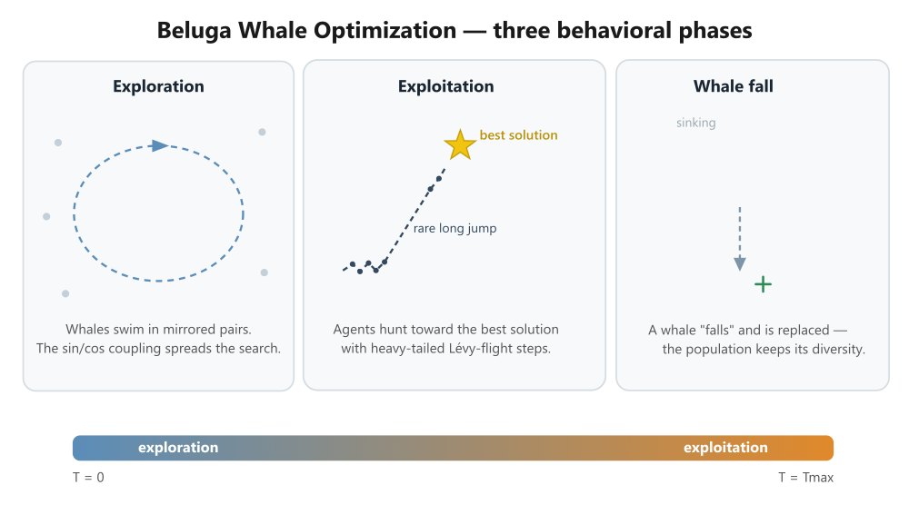
Figure 1. Phases of the BWO Algorithm
Beluga Whale Optimization — Three Behavioral Phases. The balance factor Bf shifts the dominant behavior over the course of the run; whale fall events remain rare (Wf: 0.1 → 0.05).
The illustration shows the three behavioral phases of BWO: exploration (the whales swim in mirror-image pairs; the dotted orbit with an arrow indicates synchronized movement and coverage of the space), exploitation (the whale moves toward the best solution — the gold star — along a Lévy flight path: small steps and one rare long jump), and whale fall (the individual sinks and is replaced by a new one; the green plus sign represents population renewal). At the bottom is a gradient band representing the balance factor Bf: the transition from exploration to exploitation over the course of the run, with a note that whale fall is rare and becomes less frequent.
Let's write some pseudocode for the algorithm.
BWO ALGORITHM (Beluga Whale Optimization)

INPUT: Npop — population size
       Max_it — number of iterations
       lb, ub — search bounds
       nD — task dimensionality
       fobj — objective function (minimization)

OUTPUT: xposbest, fvalbest — best solution and its value

// ---- Initialization ----
FOR each agent i = 1..Npop:
    pos[i] = rand(nD) * (ub - lb) + lb
    fit[i] = fobj(pos[i])
END
(fvalbest, index) = min(fit)
xposbest = pos[index]

// ---- Main loop ----
FOR T = 1..Max_it:

    WF = 0.1 - 0.05 * (T / Max_it)                  // probability of a whale fall

    FOR each agent i = 1..Npop:
        kk[i] = (1 - 0.5 * T / Max_it) * rand()     // balance between exploration and exploitation
    END

    // === Phase 1: Swimming / Hunting ===
    FOR each agent i = 1..Npop:
        select RJ — random agent index, RJ ≠ i

        IF kk[i] > 0.5:                             // --- EXPLORATION (pair swimming) ---
            r1 = rand();  r2 = rand()

            IF nD ≤ Npop/5:                         // Update 2 random dimensions
                (p1, p2) = two random dimension indices
                newpos[i][p1] = pos[i][p1] + (pos[RJ][p1] - pos[i][p2])*(r1+1)*sin(r2*360°)
                newpos[i][p2] = pos[i][p2] + (pos[RJ][p1] - pos[i][p2])*(r1+1)*cos(r2*360°)
            OTHERWISE:                              // Update the dimensions in pairs
                params = random dimension swap 1..nD
                FOR j = 1..floor(nD/2):
                    newpos[i][2j-1] = pos[i][params[2j-1]]
                                    + (pos[RJ][params[1]] - pos[i][params[2j-1]])*(r1+1)*sin(r2*360°)
                    newpos[i][2j]   = pos[i][params[2j]]
                                    + (pos[RJ][params[1]] - pos[i][params[2j]])*(r1+1)*cos(r2*360°)
                END
            END

        OTHERWISE:                                   // --- EXPLOITATION (hunting, Lévy flight) ---
            r3 = rand();  r4 = rand()
            C1 = 2 * r4 * (1 - T / Max_it)           // hunting intensity factor
            LevyFlight = Levy flight vector (nD), KD multiplier = 0.05
            newpos[i] = r3*xposbest - r4*pos[i] + C1 * LevyFlight ⊙ (pos[RJ] - pos[i])
        END

        newpos[i] = bound by [lb, ub]
        newfit = fobj(newpos[i])

        IF newfit < fit[i]:                          // greedy selection
            pos[i] = newpos[i];  fit[i] = newfit
        END
    END

    // === Phase 2: Whale fall ===
    FOR each agent i = 1..Npop:
        IF kk[i] ≤ WF:
            select RJ — random agent index
            r5, r6, r7 = rand()
            C2 = 2 * Npop * WF
            stepsize2 = r7 * (ub - lb) * exp(-C2 * T / Max_it)
            newpos[i] = (r5*pos[i] - r6*pos[RJ]) + stepsize2

            newpos[i] = bound by [lb, ub]
            newfit = fobj(newpos[i])
            IF newfit < fit[i]:
                pos[i] = newpos[i];  fit[i] = newfit
            END
        END
    END

    // === Global best update ===
    (fval, index) = min(fit)
    IF fval < fvalbest:
        fvalbest = fval;  xposbest = pos[index]
    END

END
RETURN xposbest, fvalbest
Let's move on to the implementation. As usual, the algorithm is implemented as a separate class that inherits from the base class C_AO. The base class provides us with all the standard features — an array of agents, storage for the best solution, and parameters — and we are required to implement four methods: SetParams, Init, Moving, and Revision.
//+------------------------------------------------------------------+
//|                  Beluga Whale Optimization                       |
//+------------------------------------------------------------------+
class C_AO_BWO : public C_AO
 {
public:
                    ~C_AO_BWO() {}
                     C_AO_BWO()
   {
    ao_name = "BWO";
    ao_desc = "Beluga Whale Optimization";
    ao_link = "https://www.mql5.com/en/users/joo";

    popSize = 30;
    KD      = 0.05;

    ArrayResize(params, 2);
    params [0].name = "popSize";
    params [0].val = popSize;
    params [1].name = "KD";
    params [1].val = KD;
   }

  void               SetParams();
  bool               Init(const double &rangeMinP [], const double &rangeMaxP [],
              const double &rangeStepP [], const int epochsP = 0);
  void               Moving();
  void               Revision();

  double             KD;                 // Lévy flight intensity (original: 0.05)

private:
  double snap_c      [];          // [popSize*coords] — population snapshot
  double snap_f      [];          // [popSize] — fitness snapshot
  int    shuf        [];          // [coords] — coordinate permutation buffer

  int                epochs, epochsDen, epochNow;   // iteration counters
  double             levySigma;                     // Lévy flight scale constant

  double             Gauss();            // standard normal random number
  double             LevyStep();         // one Lévy flight sample
 };
The parameters deserve a closer look. There are only two of them — and that is a distinctive feature of BWO: the algorithm is nearly parameter-free. popSize is the population size, which is common to all methods in the series. KD is the Lévy flight intensity; in the original paper, it is a hard-coded constant of 0.05. We exposed it as a parameter solely to make experimentation easier. The algorithm calculates everything else — the balance factor, whale fall probability, and force coefficients — during the run.
Internal buffers: snap_c and snap_f store a snapshot of the population at the start of the iteration — this is needed for greedy selection (greedy acceptance): if a new position turns out to be worse, we revert to the snapshot. shuf is a working array for permuting coordinate indices during the exploration phase. The three counters — epochs, epochsDen, and epochNow — are needed so that the algorithm can calculate the ratio T/Tmax. And levySigma is a precomputed constant for the Lévy flight.
Initialization. StandardInit sets up the basic framework, after which we randomly place the initial population — for now, into the cP array; during the very first Moving step, it will be transferred to the working coordinates. Next, we allocate buffers and set up the iteration counter.
//+------------------------------------------------------------------+
//|                              Init                                |
//+------------------------------------------------------------------+
bool C_AO_BWO::Init(const double &rangeMinP [], const double &rangeMaxP [],
                    const double &rangeStepP [], const int epochsP = 0)
 {
  if(!StandardInit(rangeMinP, rangeMaxP, rangeStepP))
    return false;

  for(int i = 0; i < popSize; i++)
    for(int c = 0; c < coords; c++)
      a [i].cP [c] = u.RNDfromCI(rangeMin [c], rangeMax [c]);

  ArrayResize(snap_c, popSize * coords);
  ArrayResize(snap_f, popSize);
  ArrayResize(shuf,   coords);

  epochs    = epochsP;
  epochsDen = (epochs > 1) ? epochs - 1 : 1;
  epochNow  = 0;

//--- sigma for Lévy flight (Mantegna), beta = 1.5
  double beta = 1.5;
  double g1   = 1.3293403881791;   // Γ(2.5)
  double g2   = 0.9064024770554;   // Γ(1.25)
  levySigma = MathPow((g1 * MathSin(M_PI * beta / 2.0)) /
                      (g2 * beta * MathPow(2.0, (beta - 1.0) / 2.0)), 1.0 / beta);
  return true;
 }
The last block requires clarification. Lévy flight using Mantegna's method uses a constant sigma that depends on the gamma function. With beta fixed at 1.5, sigma is simply a number, so the values of Γ(2.5) and Γ(1.25) are precomputed, and sigma itself is calculated once in Init (giving approximately 0.6966).
Lévy flight is implemented in two auxiliary methods:
//+------------------------------------------------------------------+
//|              Gauss — standard normal random variate (Box–Muller) |
//+------------------------------------------------------------------+
double C_AO_BWOm::Gauss()
 {
  double u1 = u.RNDfromCI(0.0, 1.0);
  double u2 = u.RNDfromCI(0.0, 1.0);
  if(u1 < 1e-15)
    u1 = 1e-15;
  return MathSqrt(-2.0 * MathLog(u1)) * MathCos(2.0 * M_PI * u2);
 }
//+------------------------------------------------------------------+
//+------------------------------------------------------------------+
//|        LevyStep — one Lévy flight sample (Mantegna)              |
//+------------------------------------------------------------------+
double C_AO_BWOm::LevyStep()
 {
  double uu = Gauss() * levySigma;
  double vv = Gauss();
  double av = MathAbs(vv);
  if(av < 1e-300)
    av = 1e-300;
  return KD * (uu / MathPow(av, 1.0 / 1.5));
 }
Moving — the core of the algorithm. Before looking at the code, here is one important caveat about the port. In the original algorithm, a single BWO iteration consists of two moves and two evaluations of the objective function: first, all whales make a swimming or hunting move; then, for a subset of individuals, the whale fall mechanism is additionally triggered. Our framework allocates exactly one function evaluation per agent per epoch. Therefore, the three behavioral models are grouped into mutually exclusive branches: during a single epoch, the whale either conducts exploration, engages in exploitation, or experiences a whale fall. The range of the balance factor is divided into intervals without gaps.
The method begins by handling the very first run and taking a snapshot:
//+------------------------------------------------------------------+
//|                            Moving                                |
//+------------------------------------------------------------------+
void C_AO_BWO::Moving()
 {
  if(!revision)                                 // First pass: cP -> c
   {
    for(int i = 0; i < popSize; i++)
      for(int c = 0; c < coords; c++)
        a [i].c [c] = u.SeInDiSp(a [i].cP [c], rangeMin [c], rangeMax [c], rangeStep [c]);
    return;
   }

  epochNow++;
  double tRatio = (double)epochNow / (double)epochsDen;   // T/Tmax ratio
  if(tRatio > 1.0)
    tRatio = 1.0;

  for(int i = 0; i < popSize; i++)               // population snapshot
   {
    for(int c = 0; c < coords; c++)
      snap_c [i * coords + c] = a [i].c [c];
    snap_f [i] = a [i].f;
   }

  double WF = 0.1 - 0.05 * tRatio;               // probability of a whale fall
In the first epoch, the population has not yet been evaluated, so we simply copy the starting coordinates into the working array and exit—the outer loop will evaluate them. For all subsequent epochs, we increment the counter, calculate the ratio T/Tmax, take a snapshot, and compute the current probability of a whale fall.
Next comes the main loop over the whales. For each one, a balance factor is calculated and a random neighbor is selected:
  for(int i = 0; i < popSize; i++)
   {
    double Bf = (1.0 - 0.5 * tRatio) * u.RNDprobab();    // balance factor

    int RJ = i;                                          // random neighbor RJ != i
    if(popSize > 1)
      while(RJ == i)
        RJ = u.RNDminusOne(popSize);
The first branch — whale fall — is triggered when Bf ≤ WF:
    if(Bf <= WF)
     {
      double r5 = u.RNDprobab(), r6 = u.RNDprobab(), r7 = u.RNDprobab();
      double C2    = 2.0 * (double)popSize * WF;
      double decay = MathExp(-C2 * tRatio);

      for(int c = 0; c < coords; c++)
       {
        double step = r7 * (rangeMax [c] - rangeMin [c]) * decay;
        double v    = r5 * snap_c [i * coords + c] -
                      r6 * snap_c [RJ * coords + c] + step;
        a [i].c [c] = u.SeInDiSp(v, rangeMin [c], rangeMax [c], rangeStep [c]);
       }
     }
The second branch — exploration through pair swimming — is triggered when Bf > 0.5. Coordinates are processed in pairs: the odd coordinate is processed using the sine function, and the even coordinate is processed using the cosine function. One of the neighbor's coordinates serves as the reference value; the coordinate indices are shuffled beforehand:
else
  if(Bf > 0.5)
   {
    double r1 = u.RNDprobab(), r2 = u.RNDprobab();
    double sinA = MathSin(2.0 * M_PI * r2);
    double cosA = MathCos(2.0 * M_PI * r2);

    for(int c = 0; c < coords; c++)            // Unaffected coordinates retain their previous values
      a [i].c [c] = snap_c [i * coords + c];

    for(int c = 0; c < coords; c++)
      shuf [c] = c;          // Fisher–Yates shuffle
    for(int c = 0; c < coords - 1; c++)
     {
      int r = c + u.RNDminusOne(coords - c);
      int t = shuf [c];
      shuf [c] = shuf [r];
      shuf [r] = t;
     }

    int    refDim = shuf [0];
    double ref    = snap_c [RJ * coords + refDim];         // ONE reference scalar
    int    pairs  = coords / 2;

    for(int j = 0; j < pairs; j++)
     {
      int dA = 2 * j, dB = 2 * j + 1;
      int pA = shuf [2 * j], pB = shuf [2 * j + 1];
      double xA = snap_c [i * coords + pA];
      double xB = snap_c [i * coords + pB];
      double vA = xA + (ref - xA) * (r1 + 1.0) * sinA;
      double vB = xB + (ref - xB) * (r1 + 1.0) * cosA;
      a [i].c [dA] = u.SeInDiSp(vA, rangeMin [dA], rangeMax [dA], rangeStep [dA]);
      a [i].c [dB] = u.SeInDiSp(vB, rangeMin [dB], rangeMax [dB], rangeStep [dB]);
     }
   }
The third branch — exploitation through hunting with a Lévy flight — is used for all other values of Bf:
else
     {
      double r3 = u.RNDprobab(), r4 = u.RNDprobab();
      double C1 = 2.0 * r4 * (1.0 - tRatio);

      for(int c = 0; c < coords; c++)
       {
        double xi = snap_c [i * coords + c];
        double xr = snap_c [RJ * coords + c];
        double Lv = LevyStep();
        double v  = r3 * cB [c] - r4 * xi + C1 * Lv * (xr - xi);
        a [i].c [c] = u.SeInDiSp(v, rangeMin [c], rangeMax [c], rangeStep [c]);
       }
     }
   }
 }
All three branches are direct ports of the formulas discussed in the previous section. We do not specify the boundary conditions separately: the SeInDiSp function, through which each new coordinate passes, also clamps it to the valid range.
Revision does two things: it updates the personal and global bests and performs greedy selection — if the whale's new position is worse than the snapshot, its coordinates and fitness are rolled back. That is precisely why the population in BWO does not deteriorate: a move may be unsuccessful, but it is not retained.
//+------------------------------------------------------------------+
//|                           Revision                               |
//+------------------------------------------------------------------+
void C_AO_BWO::Revision()
 {
  for(int i = 0; i < popSize; i++)                  // update bests
   {
    if(a [i].f > a [i].fB)
     {
      a [i].fB = a [i].f;
      ArrayCopy(a [i].cB, a [i].c, 0, 0, coords);
     }
    if(a [i].f > fB)
     {
      fB = a [i].f;
      ArrayCopy(cB, a [i].c, 0, 0, coords);
     }
   }

  if(!revision)
   {
    revision = true;
    return;
   }

  for(int i = 0; i < popSize; i++)                  // greedy acceptance: rollback if worse
    if(a [i].f < snap_f [i])
     {
      for(int c = 0; c < coords; c++)
        a [i].c [c] = snap_c [i * coords + c];
      a [i].f = snap_f [i];
     }
 }
Test Results
Let's run the standard test bench: population size of 30, a budget of 10,000 function evaluations, and 10 repetitions for each configuration.
The result is 47.51%. It would seem that we could record the result and move on to the next algorithm. But if you look not at the overall score but at how it varies with dimensionality, you will notice something strange. Look at the Hilly row: 0.6354 with 10 coordinates, 0.6083 with 50, and suddenly 0.6898 with 1,000. As the dimensionality increases, the score does not decrease but rather increases — and turns out to be higher with a thousand coordinates than with ten. For a population-based algorithm with a fixed computational budget, this is counterintuitive.
A monotonically decreasing score with respect to dimensionality is the norm — it is the nature of the process. A rise is a sign that part of the result was not obtained through search. And the stronger the rise, the louder the signal: BWO's score with 1,000 coordinates did not merely hold steady; it exceeded the result with 10 coordinates.
BWO|Beluga Whale Optimization|30.0|0.05|
=============================
5 Hilly's; Func runs: 10000; result: 0.6353865355283055
25 Hilly's; Func runs: 10000; result: 0.6082998984102445
500 Hilly's; Func runs: 10000; result: 0.6898049949555738
=============================
5 Forest's; Func runs: 10000; result: 0.42042059098839246
25 Forest's; Func runs: 10000; result: 0.34230526219017604
500 Forest's; Func runs: 10000; result: 0.34595127333449394
=============================
5 Megacity's; Func runs: 10000; result: 0.488
25 Megacity's; Func runs: 10000; result: 0.34586666666666666
500 Megacity's; Func runs: 10000; result: 0.39973333333333316
=============================
All score: 4.27577 (47.51%)
In the composite test, ten coordinates are allocated to five different functions: one pair each to Hilly, Forest, Megacity, Peaks, and Skin, with the agent's fitness being the average across all five functions. The idea is simple: any geometric trick the algorithm might pull off relies on repetition — on the fact that all pairs are structured the same way. In the composite test, the five functions have five different optima with different geometries, so such a trick can provide a gain on at most one pair out of five, and that gain is diluted in the overall score. A composite test is, in essence, a check to see if the result holds up when the geometric foundation is pulled out from under it.
BWO scored 38.57% on this test. Now let's compare. On the standard test bench, the same first functions with 10 coordinates yielded scores of 0.6354 for Hilly, 0.4204 for Forest, and 0.4880 for Megacity — an average of about 0.515. The overall score for the composite is 0.386. In other words, performance on the first functions, which looked quite respectable when tested individually, drops noticeably in the mixed configuration. And that is already a sign. A composite test does not fundamentally change the problem. It simply prevents the algorithm from exploiting the fact that the pairs are identical.
BWO|Beluga Whale Optimization |30.0|0.05|
=============================
Composite anti-cheat test: Hilly + Forest + Megacity + Peaks + Skin
Coordinates: 10; Epochs: 333; Repeats: 10
=============================
Run 1/10: 0.37161205365313077
Run 2/10: 0.40112339728582336
Run 3/10: 0.3706551427065614
Run 4/10: 0.4216333585559708
Run 5/10: 0.4101199993944876
Run 6/10: 0.3934049133990568
Run 7/10: 0.3593573524858875
Run 8/10: 0.3965450586725149
Run 9/10: 0.3584922015596293
Run 10/10: 0.3737824222225442
=============================
Average result: 0.3856725900 (38.57%)
Let's take a closer look at what exactly happens to the algorithm while it is running.
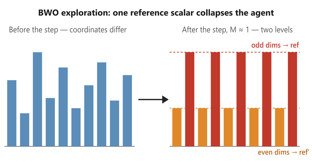
Figure 2. Coordinate collapse during exploration
During the exploration phase in BWO, a single reference scalar causes the entire agent to collapse. The multiplier M = (1 + r₁)·sin(2π·r₂) remains constant for the entire agent. When M ≈ 1, each updated coordinate becomes equal to the reference coordinate X[RJ][P1] — the vector collapses.
Autopsy, Part One: The Exploration Phase.
We have the symptoms; now we need to find the cause. Let's open Moving and examine the operators one by one. Let's start with exploration — the branch where Bf > 0.5. Here is its core, already familiar from the implementation section:
double r1 = u.RNDprobab(), r2 = u.RNDprobab();   // drawn ONCE per agent
double sinA = MathSin(2.0 * M_PI * r2);
double cosA = MathCos(2.0 * M_PI * r2);

int    refDim = shuf [0];
double ref    = snap_c [RJ * coords + refDim];   // ONE scalar for all pairs

for(int j = 0; j < pairs; j++)
 {
  double xA = snap_c [i * coords + pA];
  double vA = xA + (ref - xA) * (r1 + 1.0) * sinA;
  ...
 }
This excerpt contains two facts that, taken separately, are harmless, but together create a problem. First: the reference value ref is a single scalar — one coordinate of a random neighbor — and is the same for all pairs in the loop. Second: r1 and r2 are drawn before the loop, that is, once per agent, so sinA, cosA, and the factor (1 + r1) are constant for all coordinates of this whale.
Let's spell out what each coordinate then receives. The update formula v = x + (ref − x)·(1+r1)·sin expands into a mixture:
newpos[d] = M · ref + (1 − M) · x[d], where M = (1 + r1) · sin(2π·r2)
and M is constant for each agent (for odd coordinates; for even coordinates, the same applies with cosine). This is the key point. All odd coordinates of the whale undergo the same affine transformation, with the same M, toward the same ref. And if M is close to one, then newpos[d] = ref — for all odd coordinates at once. The whale's vector, no matter how long it is, collapses into two values: one for odd coordinates and one for even coordinates. This is clearly shown in the illustration (Figure 1): on the left is a diverse set of coordinate values; on the right, almost none of that diversity remains after a single exploration move.
Why is this a cheat specifically on our test bench? A standard test consists of N copies of the same function. The global optimum of such a problem is axisymmetric by construction: all pairs of coordinates must converge to the same point. And the BWO exploration operator pulls the whale toward precisely this axisymmetric form — a vector consisting of two repeating values. In other words, the algorithm's tendency to collapse the agent directly matches the structure of the correct answer — not because the algorithm searches effectively, but because the form of its move happens to coincide with the form of the optimum.
Why does the effect grow stronger with dimensionality — as we saw in the Hilly row? With 1,000 coordinates, each whale carries a thousand coordinate values. According to order statistics, at least one of them will almost certainly be very close to the optimal coordinate of the function. The exploration operator takes a favorable value from a neighbor and, in a single step, propagates it across half the space, while greedy selection locks in the result — after all, on a test bench with identical functions, assigning a good value to hundreds of pairs at once sharply increases average fitness. The higher the dimensionality, the larger each whale's pool of coordinates and the better the seed material for broadcasting. This explains the unnatural increase in the score.
The first modification suggests itself: remove both sources of broadcasting. Let each pair of coordinates move toward the corresponding pair in the neighbor, and let r1 and r2 be drawn anew for each pair:
for(int j = 0; j < pairs; j++)
 {
  int dA = 2 * j, dB = 2 * j + 1;

  double r1 = u.RNDprobab(), r2 = u.RNDprobab();   // for EVERY pair
  double sinA = MathSin(2.0 * M_PI * r2);
  double cosA = MathCos(2.0 * M_PI * r2);

  double xA = snap_c [i  * coords + dA];
  double refA = snap_c [RJ * coords + dA];         // the corresponding coordinate in the neighbor
  double vA = xA + (refA - xA) * (r1 + 1.0) * sinA;
  ...
 }
The geometry of pair swimming is preserved — within each pair, the sine and cosine still share a single angle and remain 90° apart — but the shared reference scalar is gone, and there is no longer a single multiplier shared across the agent. There is now nothing left that can collapse the entire vector.
Let's run the test bench again. And this is where it gets really interesting: the overall score has changed, but the profile across dimensionalities is still unhealthy — at higher dimensionalities, the algorithm continues to score suspiciously high. The exploration phase was not the only channel. Where is the second one hiding? Find out in the next section.
Autopsy, Part Two: The Exploitation Phase.
BWO exploitation phase: the r₃·cB term scans the main diagonal, as shown in the image below.
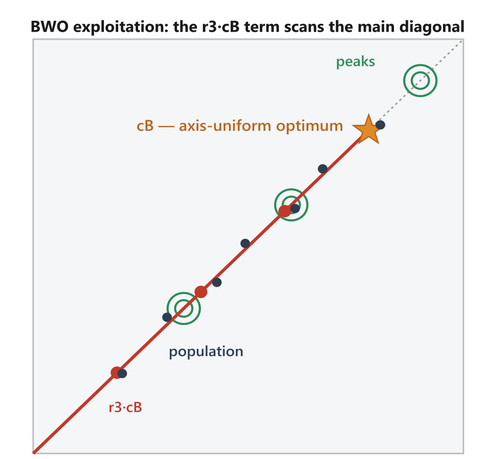
Figure 3. Diagonal Scanning in Exploitation
The red ray is r₃·cB: as r₃ varies over the range [0,1], the candidate slides along the line segment from the coordinate origin to cB. On a set of identical functions, the vector cB is axisymmetric, so this ray coincides with the main diagonal — exactly where the peaks of the objective function are located. At high dimensionality, Lévy noise averages out.
After the exploration phase was corrected, a test run showed that the anomaly had not gone away — at high dimensionality, the score was still inflated, and the algorithm was still “reading the diagonal.” So, there is more than one channel. Let's open the second branch of Moving — exploitation, where hunting involves Lévy flight:
double r3 = u.RNDprobab(), r4 = u.RNDprobab();   // r3 — ONE scalar per agent
double C1 = 2.0 * r4 * (1.0 - tRatio);

for(int c = 0; c < coords; c++)
 {
  double xi = snap_c [i * coords + c];
  double xr = snap_c [RJ * coords + c];
  double Lv = LevyStep();
  double v  = r3 * cB [c] - r4 * xi + C1 * Lv * (xr - xi);
  ...
 }
The sticking point here is the term r3·cB. This is a scalar multiplied by the vector of the global best solution. Recall that, on a test bench with identical functions, cB is axisymmetric — all of its coordinate pairs lie at the same point. And when r3 varies over the interval [0, 1], the point r3·cB slides along the ray from the coordinate origin to cB. And the ray from the coordinate origin to an axisymmetric point is precisely the main diagonal of the search space.
It only gets worse from here. As soon as the population converges on this diagonal (and it does converge because greedy selection reinforces successful moves along the ray), the position of the whale xi itself also ends up on the diagonal. Then the entire core of the move, r3·cB − r4·xi, is a linear combination of two collinear vectors, and it stays on the diagonal line. The only term that takes a candidate off the diagonal is Lévy flight.
And that is where dimensionality comes into play. Our greedy selection accepts a candidate based on its average fitness — the average Core value across all coordinate pairs. The core of the move, r3·cB − r4·xi, shifts all pairs coherently in the same direction, so it reliably shifts this average. The Lévy term, by contrast, shifts each pair in an independent random direction — and at high dimensionality, its contribution to the average cancels out to zero by the law of large numbers. Selection simply stops seeing the Lévy term. As a result, on a thousand-dimensional problem, the algorithm behaves the same way as on a one-dimensional problem: it selects r3 to scan the diagonal. The higher the dimensionality, the more effectively the Lévy noise is averaged out, and the closer the algorithm's behavior is to a pure diagonal scan. This mechanism is clearly shown in the illustration (Figure 2).
It is now clear that both channels suffer from the same underlying problem. The same pattern is to blame in both exploration and exploitation: a random multiplier drawn once per agent and multiplied by a structured vector. In exploration, this was the shared reference scalar X[RJ][P1]; here, it is r3 multiplied by cB. Any such scalar confines a candidate to a low-dimensional subspace, and on a test bench of identical functions, this subspace coincides with the diagonal, where the optimum lies. This leads to a rule for a fair modification: no random scalar drawn once per agent should multiply a meaningful vector.
Let's apply this rule. In exploitation, we remove the scalar scaling term r3·cB and implement the pull toward the best solution using coordinate-wise interpolation — each coordinate moves its own random fraction of the distance toward its corresponding cB[c]:
double r4 = u.RNDprobab();
double C1 = 2.0 * r4 * (1.0 - tRatio);

for(int c = 0; c < coords; c++)
 {
  double r3c = u.RNDprobab();                    // for EACH coordinate
  double xi  = snap_c [i * coords + c];
  double xr  = snap_c [RJ * coords + c];
  double Lv  = LevyStep();
  double v   = xi + r3c * (cB [c] - xi) + C1 * Lv * (xr - xi);
  ...
The same approach fixes the whale fall phase: the multipliers r5 and r6 become coordinate-wise so that the underlying expression r5·xi − r6·xr does not confine the candidate to the plane spanned by the two vectors:
for(int c = 0; c < coords; c++)
 {
  double r5c  = u.RNDprobab();
  double r6c  = u.RNDprobab();
  double step = r7 * (rangeMax [c] - rangeMin [c]) * decay;
  double v    = r5c * snap_c [i * coords + c] -
                r6c * snap_c [RJ * coords + c] + step;
  ...
 }
It is worth clarifying which quantities we still draw once per agent and why this does not violate the rule. The coefficients C1 (Lévy attenuation) and r7 (the magnitude of the whale fall step) are still drawn once per agent. However, they multiply not structured vectors, but vectors with coordinate-wise randomness — the Lévy vector and the relocation step. Uniform scaling of a random vector does not collapse it into a subspace or create a diagonal. Only a scalar multiplying a meaningful vector such as cB or xi confines the candidate in this way — and all three such scalars have been removed.
Let's call the resulting version BWOm. The three-phase structure, the balance factor, the probability of a whale fall, the Lévy flight, and temporal attenuation all remain unchanged; only the way randomness is drawn has changed — it is now coordinate-wise in all three phases. All that's left is to run the test bench and see what an honest performance profile looks like — we will do that in the next section.
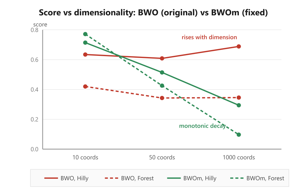
Figure 4. Profile plot by dimensionality
Test results:
BWOm|Beluga Whale Optimization (modified)|30.0|0.05|
=============================
5 Hilly's; Func runs: 10000; result: 0.7130978249513108
25 Hilly's; Func runs: 10000; result: 0.5129375854531272
500 Hilly's; Func runs: 10000; result: 0.29394203648024203
=============================
5 Forest's; Func runs: 10000; result: 0.7714504280808662
25 Forest's; Func runs: 10000; result: 0.42740547099458537
500 Forest's; Func runs: 10000; result: 0.09803668589845292
=============================
5 Megacity's; Func runs: 10000; result: 0.656
25 Megacity's; Func runs: 10000; result: 0.35386666666666666
500 Megacity's; Func runs: 10000; result: 0.13465333333333432
=============================
Total score: 3.96139 (44.02%)
Let's summarize both sets of results from the algorithm in a single table:
| Function, dimensionality | BWO (original) | BWOm (corrected) |
|---|---|---|
| Hilly, 10 | 0.635 | 0.713 |
| Hilly, 50 | 0.608 | 0.513 |
| Hilly, 1,000 | 0.690 | 0.294 |
| Forest, 10 | 0.420 | 0.771 |
| Forest, 50 | 0.342 | 0.427 |
| Forest, 1,000 | 0.346 | 0.098 |
| Megacity, 10 | 0.488 | 0.656 |
| Megacity, 50 | 0.346 | 0.354 |
| Megacity, 1,000 | 0.400 | 0.135 |
The profile by dimensionality — shown in the illustration above — now has a clear interpretation. For BWOm, the score on all three functions decreases monotonically as dimensionality increases: there is no uptick at 1,000 coordinates; the curve behaves just as it should for an honest population-based algorithm with a fixed budget. The anomaly that prompted the investigation has been resolved.
Next are two observations that I think are the most important in this whole story.
First. With 10 coordinates, BWOm outperforms the original on all three functions, and by a significant margin: Hilly 0.713 vs. 0.635, Forest 0.771 vs. 0.420, Megacity 0.656 vs. 0.488. In other words, the geometric trick did not just inflate the score at high dimensionality — it also stifled genuine search at low dimensionality, confining the whales to an axisymmetric subspace instead of allowing them to explore the full search space. By removing the cheat, we didn't take away the algorithm's power — we gave it back.
Second. With 1,000 coordinates, the picture is reversed — the honest BWOm falls below the original, especially sharply on Forest: 0.098 vs. 0.346. But BWO's score of 0.346 was itself the result of diagonal scanning. Remove that mechanism, and the true difficulty of the thousand-dimensional Forest problem under this computational budget is revealed. A score of 0.098 is not an implementation failure; it honestly reflects the difficulty of the problem.
That is why the overall score — which fell from 47.51% to 44.02% — must be interpreted correctly. This is not a regression — it is the deflation of the artificial portion of the score. BWOm earned its 44.02% through search, not through the geometry of the test bench; BWO did not earn its 47.51% that way. We received indirect confirmation right at the start: in a composite anti-cheat test, where the geometric trick does not work, the original scored 38.57% — which is much closer to BWOm’s legitimate low-dimensional numbers than to the repository’s 47.51%.
What does this mean for our ranking table? The table exists to help traders choose a tool for optimizing a trading strategy. A real-world strategy optimization problem always involves a heterogeneous landscape: stop-loss, take-profit, filter, and position size parameters differ in nature and have different optimal values. An algorithm that scored highly by using a "diagonal trick" simply won't work on a problem like this — there's nothing for the trick to latch onto. That is why the table should report the honest score. BWO, in its original form, cannot lay claim to a rightful place; BWOm, with its 44.02%, occupies a legitimate position — modest, but genuine.
And here are two more general conclusions that readers should take away from this article.
Diagnostic. A non-monotonic score as a function of dimensionality is a red flag. If, with a fixed computational budget, an algorithm performs not worse but better at higher dimensionalities, it is almost certainly not optimizing but reading the geometry of the test bench. It is worth checking the performance profile across dimensionalities for every new candidate for the table, and the composite anti-cheat test serves as a reliable second indicator here.
Mechanistic. The source of the cheat in BWO is a recurring pattern: a random scalar drawn once per agent and multiplied by a structured vector. Such a multiplier confines the candidate to a low-dimensional subspace. This is a common pitfall in the design of meta-heuristics, and now we know how to identify and address it — by replacing scalar randomness with coordinate-wise randomness.
Now we can look at the results of the anti-cheat test run: they are consistent with the main test results at the lower dimensionalities, although the values show considerable scatter.
BWOm|Beluga Whale Optimization (modified)|30.0|0.05|
=============================
Composite anti-cheat test: Hilly + Forest + Megacity + Peaks + Skin
Coordinates: 10; Epochs: 333; Repeats: 10
=============================
Run 1/10: 0.6768112016070393
Run 2/10: 0.8580079686168114
Run 3/10: 0.7773490639079661
Run 4/10: 0.6239346517249487
Run 5/10: 0.8031346429925448
Run 6/10: 0.7329426521976851
Run 7/10: 0.5579271937001347
Run 8/10: 0.7388632225403626
Run 9/10: 0.6460757525932408
Run 10/10: 0.7374171635629155
=============================
Average result: 0.7152463513 (71.52%)
=============================
Visualization of BWOm in action on the test functions, with demonstrations on several other functions as well.

BWOm on the Hilly test function

BWOm on the Forest test function

BWOm on the Megacity test function

BWOm on the Rosenbrock test function

BWOm on the Ackley test function
Before giving the algorithm a final rating, it is a good idea to spend a little time looking at the parameters — we intentionally left them as they were in the article. The default values were as follows: popSize = 30, KD = 0.05. With these settings, BWOm achieved an honest but modest 44.02%. KD = 0.05 is, in fact, not a configurable parameter, but a hard-coded Lévy flight constant from the reference implementation, and it is conservative. After we removed the geometric cheat, Lévy flight became the only long-range mechanism in the exploitation phase, and its scale directly determines the search energy. For our three multimodal functions, a value of 0.05 results in jumps that are too short.
Let's increase KD and simultaneously reduce the population — with a fixed budget of 10,000 function evaluations, a smaller population means more iterations per agent, allowing coordinate-wise interpolation toward the best solution to work one step deeper. With popSize = 20 and KD = 1.5, we get:
=============================
5 Hilly's; Func runs: 10000; result: 0.784881775284155
25 Hilly's; Func runs: 10000; result: 0.5687271425947741
500 Hilly's; Func runs: 10000; result: 0.2955752923941583
=============================
5 Forest's; Func runs: 10000; result: 0.9137000614171915
25 Forest's; Func runs: 10000; result: 0.6176092379746694
500 Forest's; Func runs: 10000; result: 0.129880770631638
=============================
5 Megacity's; Func runs: 10000; result: 0.8133333333333332
25 Megacity's; Func runs: 10000; result: 0.4994666666666667
500 Megacity's; Func runs: 10000; result: 0.1500400000000007
=============================
All score: 4.77321 (53.04%)
A composite score of 83.96% is not just "good" — it is very good: stripped of its cheat, BWOm did not just remain competitive — it moved into the upper part of the table at low dimensionality. Now let's look at the variance of the results — it is high. This is a typical signature of an algorithm with an aggressive long-jump mechanism on a multimodal landscape: either a random long Lévy flight step lands in the right basin of attraction, or it does not. The original BWO did not have that option — its diagonal trick worked consistently and always yielded the same modest figure of around 0.39. The stability was deceptive.
BWOm|Beluga Whale Optimization (modified)|20.0|1.5|
=============================
Composite anti-cheat test: Hilly + Forest + Megacity + Peaks + Skin
Coordinates: 10; Epochs: 500; Repeats: 10
=============================
Run 1/10: 0.8510959078175775
Run 2/10: 0.6776209662686439
Run 3/10: 0.6864531057459684
Run 4/10: 0.9823673728411345
Run 5/10: 0.9999793806023446
Run 6/10: 0.6755386763260092
Run 7/10: 0.9720418753408225
Run 8/10: 0.8871892660061993
Run 9/10: 0.7957332506268917
Run 10/10: 0.8675285275873976
=============================
Average result: 0.8395548329 (83.96%)
Let's look at the illustration below, which shows a direct contrast between two distributions on the same scale. Composite anti-cheat test: variation across 10 runs. BWO clusters tightly around the value of 0.39 — diagonal scanning consistently yields the same modest result. BWOm ranges from 0.68 to 1.00 and exhibits a bimodal distribution: an aggressive Lévy flight step either lands in the global basin of attraction (in one run, the value reached 0.9999).
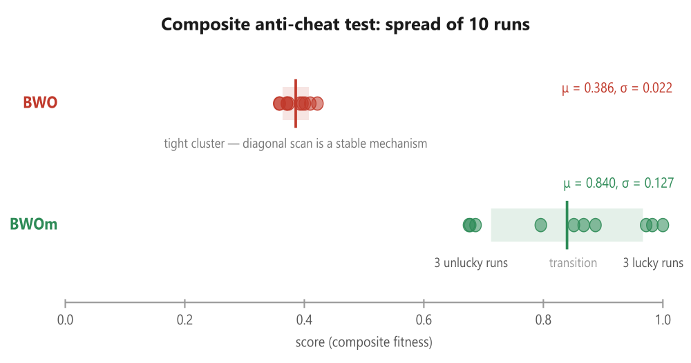
Figure 5. Spread of the two algorithms' distributions.
The top row shows ten runs of the original BWO: the data points are tightly clustered in the range of 0.36–0.42; the light band represents ±1σ (width ~5% of the scale); the vertical line indicates the mean of 0.386. Caption under the cluster: diagonal scanning is a stable mechanism — that is, the algorithm reliably obtained the same modest score from the test bench, run after run, in the anti-cheat test.
The bottom row shows ten BWOm runs: the same data points and the same ±1σ band, but now the band is six times wider — 0.71–0.97 — and three data points on the left and three on the right fall even outside its boundaries. The bimodal structure is clear: on the left is the cluster of unsuccessful runs (0.676–0.687), on the right, a cluster of successful runs (0.972–1.000); moreover, the run on the far right — which is practically at the scale limit — is the very attempt where the algorithm reached the global optimum with a result of 0.9999.
Based on the test results, the BWOm algorithm ranks 38th in our list of the best population-based optimization methods.
| cc | AO | Description | Hilly | Hilly Final | Forest | Forest Final | Megacity (discrete) | Megacity Final | Final Result | % of MAX | ||||||
| 10 p (5 F) | 50 p (25 F) | 1,000 p (500 F) | 10 p (5 F) | 50 p (25 F) | 1,000 p (500 F) | 10 p (5 F) | 50 p (25 F) | 1,000 p (500 F) | ||||||||
| 1 | ANS | across neighbourhood search | 1.00000 | 0.88228 | 0.40138 | 2.28366 | 1.00000 | 0.95281 | 0.28092 | 2.23373 | 0.94667 | 0.85733 | 0.22389 | 2.02789 | 6.545 | 72.72 |
| 2 | AMOm | animal migration optimization M | 0.91624 | 0.83603 | 0.46790 | 2.22017 | 0.98482 | 0.92010 | 0.36391 | 2.26883 | 0.91733 | 0.81707 | 0.25177 | 1.98617 | 6.475 | 71.94 |
| 3 | CLA | code lock algorithm (joo) | 0.95139 | 0.86199 | 0.37879 | 2.19217 | 0.99349 | 0.93500 | 0.26497 | 2.19346 | 0.93600 | 0.84267 | 0.24060 | 2.01927 | 6.405 | 71.17 |
| 4 | (P+O)ES | (P+O) evolution strategies | 0.86571 | 0.89539 | 0.39740 | 2.15850 | 0.97761 | 0.89820 | 0.26878 | 2.14459 | 0.92133 | 0.80240 | 0.23952 | 1.96325 | 6.266 | 69.62 |
| 5 | SDSm | stochastic diffusion search M | 0.95195 | 0.84944 | 0.36249 | 2.16388 | 0.98061 | 0.88457 | 0.22112 | 2.08630 | 0.92267 | 0.79013 | 0.21380 | 1.92660 | 6.177 | 68.63 |
| 6 | AAm | archery algorithm M | 0.84685 | 0.73320 | 0.42590 | 2.00595 | 0.96709 | 0.77837 | 0.27789 | 2.02335 | 0.86133 | 0.77707 | 0.28712 | 1.92552 | 5.955 | 66.17 |
| 7 | SIA | simulated isotropic annealing (joo) | 0.93543 | 0.86504 | 0.38483 | 2.18530 | 0.94069 | 0.80609 | 0.23835 | 1.98513 | 0.86400 | 0.66160 | 0.19536 | 1.72096 | 5.891 | 65.46 |
| 8 | TETA | time evolution travel algorithm (joo) | 0.91452 | 0.86369 | 0.25579 | 2.03400 | 0.99654 | 0.91291 | 0.14394 | 2.05339 | 0.85467 | 0.82213 | 0.10443 | 1.78123 | 5.869 | 65.21 |
| 9 | ESG | evolution of social groups (joo) | 0.98111 | 0.79857 | 0.31167 | 2.09135 | 0.98954 | 0.82270 | 0.15032 | 1.96256 | 0.92133 | 0.73440 | 0.15315 | 1.80888 | 5.863 | 65.14 |
| 10 | CTA | comet tail algorithm (joo) | 0.92435 | 0.86786 | 0.27838 | 2.07059 | 0.99039 | 0.84571 | 0.19448 | 2.03058 | 0.95467 | 0.69680 | 0.11008 | 1.76155 | 5.863 | 65.14 |
| 11 | ECBO | enhanced colliding bodies optimization | 0.94024 | 0.72363 | 0.32356 | 1.98743 | 0.99477 | 0.80291 | 0.13056 | 1.92824 | 0.87600 | 0.70160 | 0.17433 | 1.75193 | 5.668 | 62.98 |
| 12 | DA | dialectical algorithm | 0.93117 | 0.75400 | 0.26205 | 1.94722 | 0.98925 | 0.81375 | 0.08662 | 1.88962 | 0.92667 | 0.68107 | 0.11315 | 1.72089 | 5.558 | 61.76 |
| 13 | BBO | biogeography-based optimization | 0.95876 | 0.70609 | 0.35752 | 2.02237 | 0.92981 | 0.70660 | 0.16970 | 1.80611 | 0.87467 | 0.63013 | 0.20813 | 1.71293 | 5.541 | 61.57 |
| 14 | BHAm | black hole algorithm M | 0.79558 | 0.76207 | 0.34682 | 1.90447 | 0.99836 | 0.75798 | 0.13826 | 1.89460 | 0.85067 | 0.64427 | 0.17020 | 1.66514 | 5.464 | 60.71 |
| 15 | HS | harmony search | 0.91420 | 0.69049 | 0.29924 | 1.90393 | 0.97627 | 0.73373 | 0.14193 | 1.85193 | 0.91733 | 0.62720 | 0.15364 | 1.69817 | 5.454 | 60.60 |
| 16 | RFO | royal flush optimization (joo) | 0.80989 | 0.74481 | 0.34546 | 1.90016 | 0.95251 | 0.77926 | 0.15185 | 1.88362 | 0.80400 | 0.66427 | 0.19071 | 1.65898 | 5.443 | 60.48 |
| 17 | BOAm | billiards optimization algorithm M | 0.76177 | 0.72421 | 0.25275 | 1.73873 | 0.90890 | 0.81960 | 0.28853 | 2.01703 | 0.83733 | 0.74613 | 0.09763 | 1.68109 | 5.437 | 60.41 |
| 18 | ASO | anarchy society optimization | 0.73070 | 0.73713 | 0.31195 | 1.77978 | 0.99732 | 0.87700 | 0.17619 | 2.05051 | 0.72000 | 0.68773 | 0.18988 | 1.59761 | 5.428 | 60.31 |
| 19 | EOm | extremal optimization_M | 0.76527 | 0.75205 | 0.31908 | 1.83640 | 0.99999 | 0.76426 | 0.12437 | 1.88862 | 0.84133 | 0.64133 | 0.15247 | 1.63513 | 5.360 | 59.56 |
| 20 | ACS | artificial cooperative search | 0.75545 | 0.77162 | 0.31653 | 1.84360 | 1.00000 | 0.80488 | 0.10705 | 1.91193 | 0.76933 | 0.60800 | 0.14157 | 1.51890 | 5.274 | 58.60 |
| 21 | SSG | saplings sowing and growing | 0.75436 | 0.63206 | 0.35935 | 1.74577 | 0.91907 | 0.69694 | 0.19755 | 1.81356 | 0.81867 | 0.60533 | 0.21347 | 1.63747 | 5.197 | 57.74 |
| 22 | AOSm | atomic orbital search M | 0.76184 | 0.68435 | 0.31344 | 1.75963 | 0.90015 | 0.80044 | 0.11501 | 1.81560 | 0.82800 | 0.63280 | 0.15696 | 1.61776 | 5.193 | 57.70 |
| 23 | TSEA | turtle shell evolution algorithm (joo) | 0.95809 | 0.64852 | 0.29571 | 1.90232 | 0.99522 | 0.58104 | 0.10542 | 1.68168 | 0.92133 | 0.52160 | 0.14567 | 1.58860 | 5.173 | 57.48 |
| 24 | DE | differential evolution | 0.96398 | 0.62346 | 0.26089 | 1.84833 | 0.98482 | 0.77018 | 0.11459 | 1.86959 | 0.93067 | 0.36213 | 0.11000 | 1.40280 | 5.121 | 56.90 |
| 25 | BIO | blood inheritance optimization (joo) | 0.72580 | 0.66522 | 0.31228 | 1.70330 | 0.99995 | 0.68125 | 0.11540 | 1.79660 | 0.85467 | 0.59333 | 0.15364 | 1.60164 | 5.102 | 56.69 |
| 26 | (PO)ES | (PO) evolution strategies | 0.73972 | 0.58190 | 0.38896 | 1.71058 | 0.91199 | 0.59975 | 0.21262 | 1.72436 | 0.82400 | 0.56240 | 0.23432 | 1.62072 | 5.056 | 56.18 |
| 27 | BO | bonobo optimizer | 0.75555 | 0.64366 | 0.32657 | 1.72578 | 0.94332 | 0.70442 | 0.13999 | 1.78773 | 0.73467 | 0.61440 | 0.16728 | 1.51635 | 5.030 | 55.89 |
| 28 | SRA | successful restaurateur algorithm (joo) | 0.89010 | 0.63359 | 0.29115 | 1.81484 | 0.96634 | 0.55285 | 0.08914 | 1.60833 | 0.89333 | 0.52800 | 0.13911 | 1.56044 | 4.984 | 55.38 |
| 29 | CRO | chemical reaction optimisation | 0.91281 | 0.65681 | 0.29866 | 1.86828 | 0.90513 | 0.56020 | 0.10939 | 1.57472 | 0.82800 | 0.50133 | 0.14149 | 1.47082 | 4.914 | 54.60 |
| 30 | BCOm | bacterial chemotaxis optimization M | 0.82589 | 0.61733 | 0.31584 | 1.75906 | 0.95296 | 0.63718 | 0.11984 | 1.70998 | 0.76533 | 0.51653 | 0.15800 | 1.43986 | 4.909 | 54.54 |
| 31 | DOA | dream optimization algorithm | 0.78522 | 0.78121 | 0.36036 | 1.92679 | 0.61584 | 0.42117 | 0.12254 | 1.15955 | 0.86667 | 0.72587 | 0.21127 | 1.80381 | 4.890 | 54.33 |
| 32 | ABO | african buffalo optimization | 0.92295 | 0.62528 | 0.29885 | 1.84708 | 0.92992 | 0.57468 | 0.09372 | 1.59832 | 0.73333 | 0.51333 | 0.14324 | 1.38990 | 4.835 | 53.72 |
| 33 | BSA | bird swarm algorithm | 0.94432 | 0.67941 | 0.26401 | 1.88774 | 0.91649 | 0.65619 | 0.12054 | 1.69322 | 0.80933 | 0.33547 | 0.10652 | 1.25132 | 4.832 | 53.69 |
| 34 | TSm | tabu search M | 0.87806 | 0.61040 | 0.28993 | 1.77839 | 0.98116 | 0.52165 | 0.08544 | 1.58825 | 0.82667 | 0.49547 | 0.13552 | 1.45766 | 4.824 | 53.60 |
| 35 | BSA | backtracking search algorithm | 0.87128 | 0.53190 | 0.28675 | 1.68993 | 0.92408 | 0.51602 | 0.09153 | 1.53163 | 0.96000 | 0.47253 | 0.13760 | 1.57013 | 4.792 | 53.24 |
| 38 | BWOm | beluga_whale_optimization_M | 0.78488 | 0.56872 | 0.29557 | 1.64917 | 0.91370 | 0.61760 | 0.12988 | 1.66118 | 0.81333 | 0.49946 | 0.15004 | 1.46283 | 4.773 | 53.04 |
| 36 | WOAm | whale optimization algorithm M | 0.93893 | 0.59477 | 0.26695 | 1.80065 | 0.98036 | 0.53873 | 0.07112 | 1.59021 | 0.78667 | 0.47600 | 0.11892 | 1.38159 | 4.772 | 53.02 |
| 37 | ACA | andean_condor_algorithm | 0.78444 | 0.53260 | 0.33108 | 1.64812 | 0.79071 | 0.44960 | 0.10685 | 1.34716 | 0.92266 | 0.67733 | 0.17613 | 1.77612 | 4.771 | 53.02 |
| 39 | CSO | competitive swarm optimizer | 0.85151 | 0.60786 | 0.29896 | 1.75833 | 0.84085 | 0.58491 | 0.11974 | 1.54550 | 0.80000 | 0.48560 | 0.14184 | 1.42744 | 4.731 | 52.57 |
| 40 | FBA | fractal-based algorithm | 0.69419 | 0.64267 | 0.28955 | 1.62641 | 0.99812 | 0.54905 | 0.08705 | 1.63422 | 0.76133 | 0.51253 | 0.13689 | 1.41075 | 4.671 | 51.90 |
| 41 | ECOi | eco-inspired evolutionary algorithm | 0.78817 | 0.54402 | 0.29360 | 1.62579 | 0.88996 | 0.46592 | 0.09747 | 1.45335 | 0.78533 | 0.45173 | 0.14295 | 1.38001 | 4.459 | 49.54 |
| 42 | BSO | brain storm optimization | 0.92207 | 0.57625 | 0.29732 | 1.79564 | 0.80764 | 0.42508 | 0.09448 | 1.32720 | 0.77200 | 0.36533 | 0.13065 | 1.26798 | 4.391 | 48.79 |
| 43 | CAm | camel algorithm M | 0.71534 | 0.56917 | 0.35985 | 1.64436 | 0.84094 | 0.47174 | 0.10850 | 1.42118 | 0.70400 | 0.41947 | 0.19563 | 1.31910 | 4.385 | 48.72 |
| 44 | ACOm | ant colony optimization_M | 0.71885 | 0.48410 | 0.30990 | 1.51285 | 0.75792 | 0.48639 | 0.11871 | 1.36302 | 0.83600 | 0.48667 | 0.16148 | 1.48415 | 4.360 | 48.44 |
| 45 | BSO | brain storm optimization | 0.91331 | 0.55813 | 0.29705 | 1.76849 | 0.85329 | 0.44038 | 0.09447 | 1.38814 | 0.72267 | 0.32880 | 0.13325 | 1.18472 | 4.341 | 48.23 |
| RW | random walk | 0.49970 | 0.32333 | 0.25791 | 1.08094 | 0.30754 | 0.11470 | 0.04400 | 0.46624 | 0.36133 | 0.17013 | 0.10244 | 0.63390 | 2.181 | 24.23 | |
Conclusions
So, the overall score rose from 44.02% to 53.04% — that puts it firmly in the upper-middle range of the rankings. The performance profile as a function of dimensionality remained monotonically decreasing across all three functions — that is, there were no gains from any new artifacts; we simply ended up with a better-tuned, honest optimizer. And at low dimensionality, the results are strong: Hilly 0.78, Forest 0.91, Megacity 0.81 — these are impressive figures.
The composite anti-cheat test, using the same settings, yielded a result of 83.96%. Let's take a moment to look closely at this number. For 10 coordinates, the standard test bench averaged BWOm's scores across the three functions as (0.7849 + 0.9137 + 0.8133)/3 ≈ 0.8373. The composite test with the same 10 coordinates, but consisting of five different functions with different optima, yields 0.8396. The two values are almost identical. This is the hallmark of honest optimization: with the same budget and dimensionality, the algorithm performs just as well on a homogeneous landscape as it does on a heterogeneous one — because it does not exploit the shape of the test bench, but actually searches. The original BWO showed a drop from 47.51% to 38.57% here; BWOm shows no such drop.
Strengths. The key point is that, after refinement, the algorithm produces honest results and performs well where it really matters for the practical optimization of trading strategies: at low and medium dimensionality. Only a few of the methods listed in the table are capable of yielding a value of 0.83 on a homogeneous benchmark and 0.84 on a composite benchmark at the same time. The performance profile as a function of dimensionality behaves as expected, with no upturns or anomalies. There are only two parameters to configure — popSize and KD — which means the algorithm is easy to use, and KD has also proven to be a useful, adjustable parameter rather than the fixed value of 0.05 mentioned in the article. Conceptually, the design is also appealing: three qualitatively different operators with smooth switching between them controlled by the balance factor, plus Lévy flight, which provides rare but critical long-range jumps to escape local optima.
Weaknesses. The main weakness is a sharp decline in performance as dimensionality increases. With 1,000 coordinates, Forest scores only 0.13 and Megacity 0.15 — that is no longer top-ranking performance, but a modest mid-table showing. The coordinate-wise randomness we introduced in all three phases during the revision does not, by design, inflate the mean through pair-averaged acceptance; on thousand-dimensional problems with a fixed budget, this is not enough. So BWOm is not a suitable choice for optimization problems with hundreds of parameters. The second drawback is the whale fall phase. It is rare (Wf does not exceed 0.1 and tapers off to 0.05), and its contribution to the overall dynamics is small; in some tests, it could be disabled with almost no loss, which slightly diminishes its role in the concept. The third drawback is the legacy of the original. The published algorithm in its original form cheats, and without understanding where and why, you could enter an unjustified figure of 47.51% in the table. That is actually the whole point of this analysis.
Where to use it. For a typical trader's task — optimizing a strategy with anywhere from a handful to several dozen parameters — BWOm is one option in our table: low dimensionality, a heterogeneous parameter landscape (stop-loss levels, take-profit levels, filters, ATR multipliers—all different in nature), and the need to escape local optima. Lévy flight and honest coordinate-wise search come into their own here. However, if a strategy is highly parameterized (hundreds of neural network weights, thousands of variables in a portfolio problem), BWOm will be outperformed by specialized high-dimensional methods — and in this case, it makes sense to look at the top rows of the table for the corresponding category.
Practical implications for traders. An algorithm in which 30% of runs fall 16–18 percentage points below the average cannot be run just once and trusted to yield reliable results — a multi-restart strategy is required. Running BWOm with three to five independent initializations and selecting the best result virtually guarantees a result in the upper part of the distribution (the probability of not getting a single successful run out of five, given a success rate of ~70%, is approximately 0.3⁵ ≈ 0.2%). For a serious strategy optimization task, 3–5 restarts are a drop in the bucket; they do not make any difference to the overall computation budget. But without restarts, a lone score of 0.68 on a real-world problem leaves the trader wondering whether the strategy is weak or the optimizer fell short — and that is a bad position to be in.
In the next article, we will examine another candidate for the table — and the tools we have acquired here (checking the performance profile across dimensionalities, the composite anti-cheat test, and the rule against per-agent scalars multiplying a structured vector) will be put to work from the very first line.
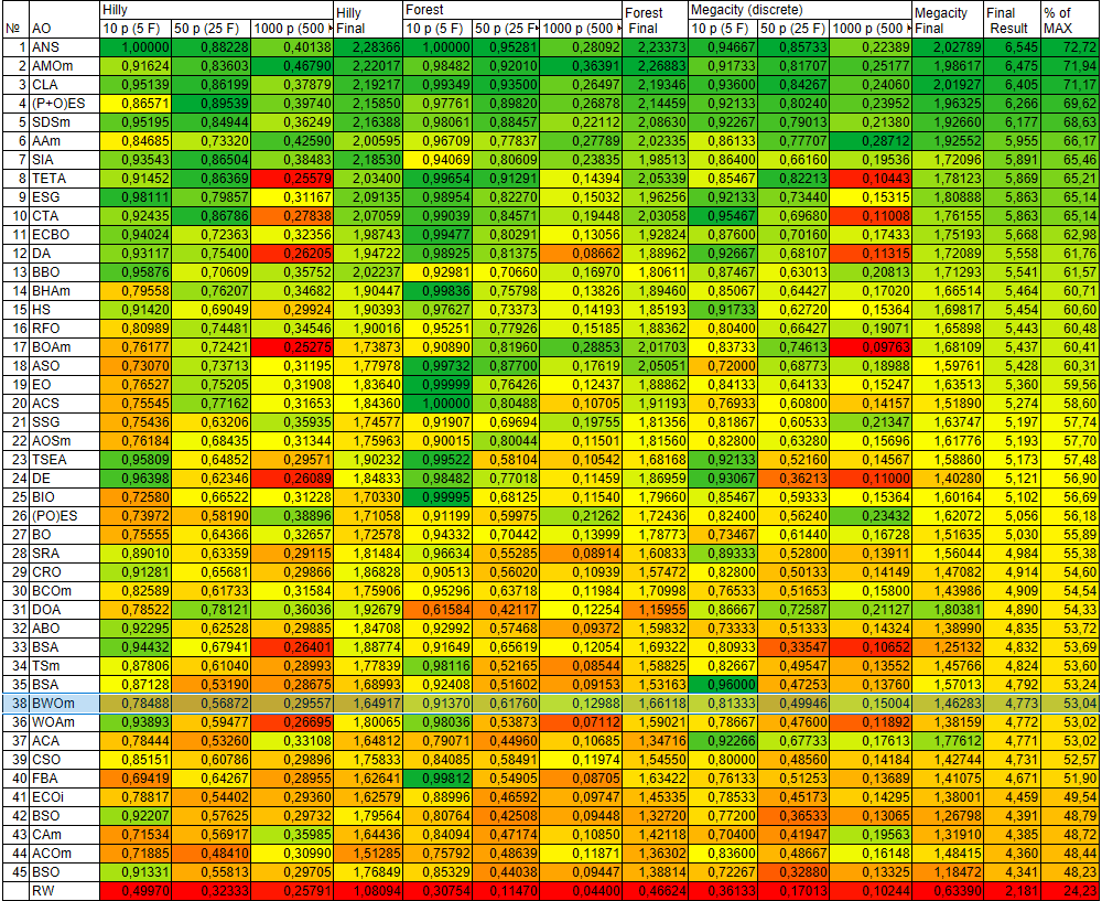
Figure 6. Color-coded ranking of algorithms based on the corresponding tests
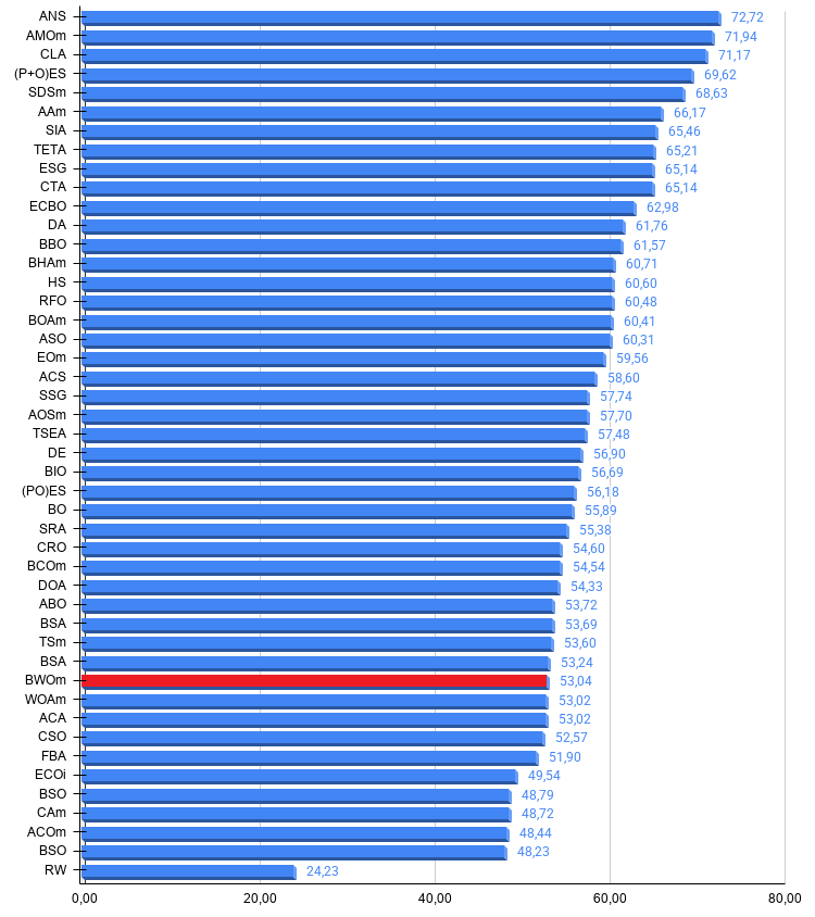
Figure 7. A histogram of the algorithm test results (on a scale from 0 to 100; the higher the score, the better, where 100 is the maximum possible theoretical result); the archive contains a script for calculating the ranking table
Pros and cons of the BWOm algorithm:
Pros:
- A small number of external parameters.
- Fast.
Cons:
- Prone to stagnation.
An archive containing the latest versions of the algorithm source code is attached to the article. The author of this article accepts no responsibility for the absolute accuracy of the descriptions of canonical algorithms; many of them have been modified to improve their search capabilities. The conclusions and judgments presented in the articles are based on the results of the experiments conducted.
Software used in this article
| # | Name | Type | Description |
|---|---|---|---|
| 1 | #C_AO.mqh | Include file | Parent class of population-based optimization algorithms |
| 2 | #C_AO_enum.mqh | Include file | Enumeration of population-based optimization algorithms |
| 3 | TestFunctions.mqh | Include file | Test function library |
| 4 | TestStandFunctions.mqh | Include file | Test bench function library |
| 5 | TestStand3D.mqh | Include file | 3D visualization panel for a test bench |
| 6 | Utilities.mqh | Include file | Utility functions library |
| 7 | CalculationTestResults.mqh | Include file | Script for calculating results for the comparison table |
| 8 | Test_AO_All.mq5 | Script | Unified test bench for all population-based optimization algorithms |
| 9 | Test_AO_AntiCheat | Script | Anti-cheat test for optimization algorithms |
| 10 | Simple use of population optimization algorithms.mq5 | Script | Simple example of using population-based optimization algorithms without visualization |
| 11 | Test_AO_BWOm.mq5 | Script | Test bench for BWOm |
Translated from Russian by MetaQuotes Ltd.
Original article: https://www.mql5.com/ru/articles/22686
Warning: All rights to these materials are reserved by MetaQuotes Ltd. Copying or reprinting of these materials in whole or in part is prohibited.
This article was written by a user of the site and reflects their personal views. MetaQuotes Ltd is not responsible for the accuracy of the information presented, nor for any consequences resulting from the use of the solutions, strategies or recommendations described.