Enhanced Colliding Bodies Optimization (ECBO)

Table of Contents

1. Introduction
2. Implementation of the Algorithm
3. Test Results
4. Conclusions

Introduction

Over the course of several articles, we have examined optimization algorithms that did not make it into our ranking table due to their poor search performance. In this article, we will examine a method that shows great promise for changing this trend.

Colliding Bodies Optimization (CBO) is a metaheuristic optimization algorithm developed by Kaveh and Mahdavi in 2014. The algorithm draws inspiration from the physics of one-dimensional collisions between bodies, where each potential solution to the optimization problem is represented as a physical body with mass and velocity. Just as two objects in the real world exchange momentum and energy when they collide, candidate solutions in the CBO algorithm collide with one another, exchanging information about their positions in the search space and thereby guiding the search toward the optimum.

The physical metaphor for the algorithm is based on the well-known laws of conservation of momentum and energy. Consider two billiard balls: when a moving ball strikes a stationary one, both balls acquire new velocities after the collision, depending on their masses and initial velocities. At the same time, a heavier ball is harder to set in motion, while a lighter ball receives a greater impulse. It is precisely this intuition that underlies CBO: good solutions — that is, solutions with more favorable objective-function values — gain greater mass and exert a greater influence on the direction of the search, drawing poor solutions toward them.

Implementation of the Algorithm

The algorithm begins by initializing a population of "n" bodies, where "n" must be an even number. The initial position of each body in the j-dimensional search space is set at random:

Xij = Xj,min + rand * (Xj,max - Xj,min); where Xij is the j-th coordinate of the i-th body, Xj,min and Xj,max are the search-space bounds along the j-th coordinate, and rand is a random number uniformly distributed in the interval [0, 1].

After calculating the value of the objective function "Jk" for each body, its mass is determined. In the CBO algorithm, the mass of a body is inversely proportional to the value of the objective function (for a minimization problem), which means that the better the solution, the greater its mass:

Mk = (1 / Jk) / sum_{i=1..n} (1 / Ji), k = 1, …, n

This normalization ensures that the sum of all masses equals one, and that the relative masses reflect the relative quality of the solutions.

Let's look at how the algorithm works using a specific example. Suppose we are looking for the minimum of a function on the interval from 0 to 10, and we have a population of six bodies with positions 2, 4, 5, 6, 7, and 9. After calculating the objective function for each position, the algorithm sorts the bodies by solution quality. Suppose that after sorting, the order is as follows: 5, 6, 4, 7, 2, 9 — where position 5 yields the best function value, and position 9 yields the worst. Now the population is divided in half: the first three bodies (5, 6, 4) become stationary bodies, and the remaining three (7, 2, 9) become moving bodies. Stationary bodies represent the better half of the population and remain motionless until a collision occurs, while moving bodies from the worse half move toward their stationary partners.

Pairing is based on rank matching: the best moving body (position 7, fourth in quality) collides with the best stationary body (position 5, first in quality), the second moving body (position 2) collides with the second stationary body (position 6), and the third moving body (position 9) collides with the third stationary body (position 4). This pairing ensures that the worst solutions are directed toward the best ones, rather than toward random points in the search space.

The velocities of the bodies before the collision are determined as follows. Stationary bodies are motionless:

Vi = 0, i = 1, …, n/2

The velocity of a moving body is directed toward its paired stationary body and is equal to the difference between their positions:

Vi = X_{i-(n/2)} - Xi, i = n/2 + 1, …, n

In our example, for the pair (5, 7), the velocity of the moving body is V = 5 - 7 = -2, which means movement to the left along the number line toward the stationary partner.

After the collision, the velocities of both bodies are recalculated using formulas based on the laws of conservation of momentum. For stationary bodies, the new velocity is calculated as:

V'_i = (M_{i+n/2} + epsilon * M_{i+n/2}) * V_{i+n/2} / (M_i + M_{i+n/2}), i = 1, …, n/2

For moving bodies, the formula is:

V'_i = (M_i - epsilon * M_{i-n/2}) * V_i / (M_i + M_{i-n/2}), i = n/2 + 1, …, n

where epsilon is the coefficient of restitution that determines the nature of the collision.

The coefficient of restitution is a parameter borrowed from collision physics that determines what fraction of kinetic energy is conserved after an impact. In classical mechanics, it is defined as the ratio of the relative velocities of the bodies after and before the collision:

epsilon = |V'_{i+1} - V'_i| / |V_{i+1} - V_i|

In the CBO algorithm, this coefficient plays a key role in striking a balance between exploration of the search space and exploitation of the solutions found. The value of the coefficient decreases linearly from one to zero throughout the optimization process:

epsilon = 1 - iter / iter_max

At the beginning of the optimization, the coefficient of restitution is equal to one, which corresponds to a perfectly elastic collision with complete conservation of energy — the bodies fly far apart, enabling broad exploration of the search space. As the optimization progresses, the coefficient tends toward zero, which corresponds to a perfectly inelastic collision — the bodies stick together, concentrating around the good solutions found and performing fine-tuning.

After the new velocities are calculated, the new positions of the bodies are determined. This is where an important feature of the algorithm comes into play. Stationary bodies update their position relative to their current position:

X_i^new = X_i + rand * V'_i, i = 1, …, n/2

Moving bodies update their position not relative to themselves, but relative to their stationary collision partner:

X_i^new = X_{i-n/2} + rand * V'_i, i = n/2 + 1, …, n;

where rand is a random vector with components uniformly distributed over the interval [-1, 1]. This is the key mechanism that ensures the worst solutions are drawn toward the best ones: a moving body effectively jumps into the vicinity of a stationary body, rather than simply moving in its direction.

Let's continue with our numerical example. Let the mass of the body at position 5 be 0.3, and the mass of the body at position 7 be 0.1 (smaller because the solution is worse). The coefficient of restitution for the current iteration is 0.8. The velocity of the moving body before the collision: V = 5 - 7 = -2. After the collision, the stationary body at position 5 acquires the following velocity:

Vstat' = (0.1 + 0.8 * 0.1) * (-2) / (0.3 + 0.1) = (0.18 * -2) / 0.4 = -0.9.

The moving body receives the following velocity:

Vmov' = (0.1 - 0.8 * 0.3) * (-2) / (0.3 + 0.1) = (-0.14 * -2) / 0.4 = 0.7.

Next, random numbers are generated from the interval [-1, 1]; for example, 0.6 and -0.4. New position of the stationary body:

Xstatnew = 5 + 0.6 * (-0.9) = 4.46.

The new position of the moving body is calculated relative to its stationary partner:

Xmovnew = 5 + (-0.4) * 0.7 = 4.72.

As we can see, both bodies are now near position 5, which corresponded to the best solution.

Enhanced CBO (ECBO) is an improved version of the basic algorithm that includes two additional mechanisms: Colliding Memory and crossover. Colliding Memory (CM) is a fixed-size archive that stores the best solutions found during the entire runtime of the algorithm. Before each iteration, the worst solutions in the current population are replaced with solutions from this archive. This elitism mechanism ensures that the quality of the best solution never deteriorates from one iteration to the next, and prevents the loss of valuable information about promising areas of the search space.

Let's suppose that on the tenth iteration, the algorithm found a very good solution at position 3.7, but on subsequent iterations, random perturbations drove the population into a different region. Without Colliding Memory, this solution might have been lost. Using the Colliding Memory, position 3.7 is stored in the archive and, at each iteration, is returned to the population, replacing the worst current solution. This ensures that the best points found remain in the population at all times and allows the algorithm to continue exploring their neighborhoods.

The crossover mechanism in ECBO adds an element of random diversification. After updating the positions, the following check is performed for each body:

Xij = Xj,min + rand * (Xj,max - Xj,min), if RANi < PRO; otherwise Xij;

where Xij is the randomly selected jth coordinate of the ith body, PRO is the crossover probability specified by the user in the range [0, 1], and RANi is a random number generated for each body.

This simple mechanism helps the algorithm avoid premature convergence and getting stuck in local optima by periodically relocating individual solutions to unexplored regions of the search space. The crossover probability is typically set to a low value, in the range of 0.1–0.3, so as not to disrupt the algorithm's core logic while still ensuring sufficient diversification.

One of the main advantages of CBO and ECBO is the minimal number of tunable parameters. The basic CBO does not require any configuration of internal parameters — you only need to specify the population size, which must be an even number. The coefficient of restitution is calculated automatically based on the current iteration number. ECBO adds two optional parameters: the Colliding Memory size and the crossover probability, but both have reasonable default values (one memory element and a zero crossover probability turn ECBO into a basic CBO with elitism). This simplicity sets the algorithm apart from many other metaheuristics, which require careful tuning of numerous hyperparameters.

The algorithm demonstrates a natural balance between global exploration and local exploitation thanks to its adaptive coefficient of restitution. In early iterations, when "epsilon" is close to one, the bodies scatter over large distances after collisions, effectively exploring the search space. As the optimization nears its end, "epsilon" tends toward zero, and the bodies begin to concentrate around the good solutions that have been found, refining them locally. This mechanism requires no configuration and works automatically for any task.

The computational complexity of a single CBO iteration is determined primarily by the sorting of the population, which requires O(n log n) operations, where n is the size of the population. The remaining operations — calculating masses, velocities, and new positions — are performed in linear time O(n). This makes the algorithm computationally efficient and applicable to problems involving costly objective function evaluations, where the main computational cost lies in assessing the quality of solutions rather than in the optimizer’s internal logic. Let us illustrate the operating principle of the CBO algorithm in a figure.

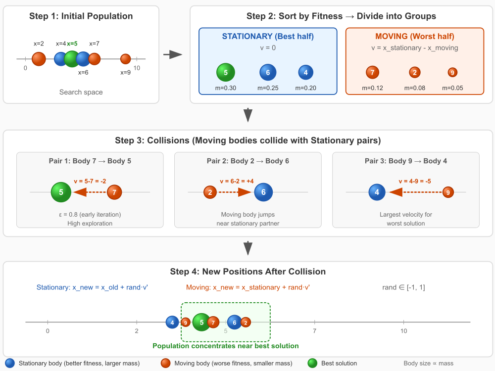
Figure 1. Illustration of the CBO algorithm in operation

The illustration shows the four main stages of CBO operation:

• Step 1 — The initial population is randomly distributed throughout the search space.
• Step 2 — After fitness is calculated, the bodies are sorted and divided into two groups: stationary bodies (the best half, blue) and moving bodies (the worst half, orange). The size of a body is proportional to its mass.
• Step 3 — Three collision pairs are shown. Moving bodies are directed toward their stationary partners; their velocity is equal to the difference between their positions.
• Step 4 — After the collisions, the entire population concentrates around the best solution (the green zone). Key point: moving bodies jump to the stationary partner's position; they do not simply shift.

Let us write pseudocode for the ECBO (Enhanced Colliding Bodies Optimization) algorithm and continue working with it, as it offers a more advanced approach to optimization.

1. Set the algorithm parameters: population size — n, dimensionality — d, Colliding Memory size — CMsize, crossover probability — PRO, number of iterations — maxIter.

2. For each body i from 1 to n: for each coordinate j from 1 to d, assign a random value within the search-space bounds.

3. For each Colliding Memory element m from 1 to CMsize: set the fitness to negative infinity.

4. Set the global best fitness to negative infinity.

5. For each body i from 1 to n: compute the fitness; if it is better than the global best, update the global best solution.

6. For each iteration iter from 1 to maxIter, perform steps 7–22.

7. For each body i from 1 to n: find the worst element in the Colliding Memory; if the body's fitness is better, replace the worst element in the Colliding Memory with the current body.

8. For each memory element m from 1 to CMsize: find the worst body in the population; if the memory element is better, replace the worst body with the memory element.

9. Sort the population in descending order of fitness.

10. Find the minimum fitness in the population.

11. If the minimum fitness is nonpositive, calculate the shift as the absolute value of the minimum plus a small constant; otherwise, the shift is zero.

12. Calculate the sum of the shifted fitness values for all bodies.

13. For each body i from 1 to n: calculate the mass as the ratio of the shifted fitness to the sum.

14. For each body i from 1 to n: save the current position as the old position.

15. Calculate the coefficient of restitution as 1 minus iter divided by maxIter.

16. For each body i from 1 to n, perform steps 17–21.

17. If i is less than or equal to n/2: set the index of the paired moving body to i plus n/2; calculate the pre-collision velocity as the current body’s old position minus the partner’s old position; calculate the post-collision velocity using the formula for stationary bodies; calculate the new position as the old position plus a random number between -1 and 1 multiplied by the post-collision velocity.

18. If i is greater than n/2: set the index of the paired stationary body to i minus n/2; calculate the pre-collision velocity as the partner’s old position minus the current body’s old position; calculate the post-collision velocity using the formula for moving bodies; calculate the new position as the paired stationary body’s old position plus a random number between -1 and 1 multiplied by the post-collision velocity.

19. Generate a random number; if it is less than PRO, select a random coordinate and assign it a random value within the bounds.

20. For each coordinate j from 1 to d: if the value is less than the minimum, set it equal to the minimum; if it is greater than the maximum, set it equal to the maximum.

21. Calculate the body's fitness; if it is better than the global best, update the global best solution.

22. Proceed to the next iteration.

23. Return the global best solution and its fitness.

Now we can move on to the code implementation itself.

The C_AO_ECBO class inherits from the base class C_AO and implements the Enhanced Colliding Bodies Optimization algorithm. The default population size is set to 50 individuals, as usual. The algorithm has three configurable parameters:

• popSize — determines the population size and must be an even number so it can be correctly divided into stationary and moving bodies;
• CMsize — specifies the size of the Colliding Memory and defaults to 20, which means that the twenty best solutions found are saved;
• PRO represents the crossover probability and is set to 0.7, ensuring sufficient diversification of the search.

Among the private members of the class are the variables "epochs" and "epochNow," which track the total number of optimization epochs and the number of the current epoch, respectively — these values are necessary for calculating the coefficient of restitution, which decreases linearly from one to zero. The "CM" array of type S_AO_Agent serves as Colliding Memory and stores the best positions found throughout the algorithm's execution. The temporary array "pTemp" is used by the sorting function to order the population by fitness value. The "mass" array stores the calculated masses of all bodies in the population.

//————————————————————————————————————————————————————————————————————
class C_AO_ECBO : public C_AO
{
  public:
  ~C_AO_ECBO () { }

  C_AO_ECBO ()
  {
    ao_name = "ECBO";
    ao_desc = "Enhanced Colliding Bodies Optimization";
    ao_link = "https://www.mql5.com/en/articles/21147";

    popSize = 50;

    ArrayResize (params, 3);
    params [0].name = "popSize";  params [0].val = popSize;
    params [1].name = "CMsize";   params [1].val = 20;    // Colliding Memory size
    params [2].name = "PRO";      params [2].val = 0.7;   // crossover probability
  }

  void SetParams ()
  {
    popSize = (int)params [0].val;
    CMsize  = (int)params [1].val;
    PRO     = params [2].val;
  }

  bool Init (const double &rangeMinP  [],
             const double &rangeMaxP  [],
             const double &rangeStepP [],
             const int     epochsP = 0);

  void Moving   ();
  void Revision ();

  //------------------------------------------------------------------
  int    CMsize;       // Colliding Memory size
  double PRO;          // crossover probability

  private: //—————————————————————————————————————————————————————————
  int    epochs;       // total number of epochs
  int    epochNow;     // current epoch

  S_AO_Agent CM     []; // Colliding Memory — stores the best positions
  S_AO_Agent pTemp  []; // temporary array for sorting

  double mass [];       // body masses

  void CalculateMasses ();
};
//————————————————————————————————————————————————————————————————————

The Init method initializes the algorithm before optimization begins. First, the base class' StandardInit method is called; it allocates memory for the coordinate arrays, sets the search-space bounds, and initializes the agent population. Next, the population size is checked to see if it is even — if popSize is odd, it is increased by one, since the algorithm requires the population to be divided into two equal groups. The total number of epochs specified by the "epochsP" parameter is stored, and the current epoch counter is reset to zero.

Next, the Colliding Memory is initialized: for each of the CMsize elements, memory is allocated for the coordinates, and the initial fitness value is set to negative infinity, which ensures that these elements are replaced by any real solutions during the initial iterations. Similarly, a temporary array of "popSize" elements is initialized for sorting. The "mass" array is also initialized — each mass is set to 1/popSize, ensuring a uniform distribution until the actual masses are calculated for the first time.

//————————————————————————————————————————————————————————————————————
bool C_AO_ECBO::Init (const double &rangeMinP  [],
                      const double &rangeMaxP  [],
                      const double &rangeStepP [],
                      const int     epochsP = 0)
{
  if (!StandardInit (rangeMinP, rangeMaxP, rangeStepP)) return false;

  //------------------------------------------------------------------
  // popSize must be even
  //------------------------------------------------------------------
  if (popSize % 2 != 0) popSize++;

  epochs   = epochsP;
  epochNow = 0;

  //------------------------------------------------------------------
  // Initializing Colliding Memory
  //------------------------------------------------------------------
  ArrayResize (CM, CMsize);
  for (int i = 0; i < CMsize; i++)
  {
    CM [i].Init (coords);
    CM [i].f = -DBL_MAX;
  }

  //------------------------------------------------------------------
  // Temporary array for sorting
  //------------------------------------------------------------------
  ArrayResize (pTemp, popSize);
  for (int i = 0; i < popSize; i++) pTemp [i].Init (coords);

  //------------------------------------------------------------------
  // Mass array
  //------------------------------------------------------------------
  ArrayResize (mass, popSize);
  for (int i = 0; i < popSize; i++) mass [i] = 1.0 / popSize;

  return true;
}
//————————————————————————————————————————————————————————————————————

The Moving method is responsible for moving all bodies in the population to new positions according to collision physics. At the beginning of the method, the "epochNow" counter is incremented. If the "revision" flag is set to 'false' — which indicates the first iteration before fitness values are obtained — all positions are randomly initialized according to formula (1): each coordinate of each body is assigned a random value uniformly distributed between the minimum and maximum search-space bounds. After the "SeInDiSp" function has discretized the values, the method terminates, leaving the collision calculation for subsequent iterations.

In subsequent iterations, when "revision" is 'true', the algorithm first saves the current positions of all bodies to the "cP" array (previous coordinates). This is a critically important step, since collision calculation must use the positions of the bodies before the update begins, rather than values that have already been modified. Next, the coefficient of restitution "epsilon" is calculated using the formula $\varepsilon = 1 - iter/iter_{max}$​. The value is clamped to the range from zero to one to prevent it from going out of bounds if the counter values are incorrect. The "halfPop" variable stores half the population size for easy indexing.

The main loop iterates through all the bodies in the population. For each body and each coordinate, a new position is calculated based on collision physics. The logic branches depending on whether the body belongs to the stationary or moving group. Bodies with indices ranging from "0" to "halfPop-1" are stationary — they represent the best half of the population after sorting. For a stationary body with index "i", its paired moving body is the body with index "i+halfPop." The velocity of a moving body before a collision is calculated as the difference between the positions of the stationary body and the moving body: vMoving = a[i].cP[c] - a[movingIdx].cP[c].

The velocity of the stationary body after a collision is determined by formula (5), where the numerator contains the product of the moving body's velocity and the sum of the moving body's mass and that same mass multiplied by "epsilon", and the denominator is the sum of the masses of both bodies. The new position of the stationary body is calculated using formula (8): the product of a random number from the range [-1, 1] and the calculated velocity is added to the old position.

The bodies with indices ranging from "halfPop" to "popSize-1" are moving — they represent the worst half of the population. For a moving body with index "i", its paired stationary body is the body with index "i-halfPop". The pre-collision velocity is calculated in the same way, but using the correct indices. The velocity after a collision is determined by formula (6), which differs from the formula for stationary bodies in the sign before "epsilon": the numerator contains the difference between the mass of the moving body and the product of "epsilon" and the mass of the stationary body. The key difference in equation (9) for the new position of a moving body is that it is measured not from the body's own position, but from the position of its paired stationary body. This causes the moving body to “jump” into the vicinity of the best solution.

After calculating the new position for each body, the crossover mechanism specific to the ECBO version is applied. A random number "ran_i" is generated, and if it is less than the crossover probability "PRO", a random coordinate "j" is selected and reinitialized with a random value from the valid range. This mechanism introduces an element of randomness that helps the algorithm avoid getting stuck in local optima. At the end of processing each body, a boundary check is performed: coordinates that fall outside the search-space bounds are clipped to the boundary values, after which discretization is applied.

//————————————————————————————————————————————————————————————————————
void C_AO_ECBO::Moving ()
{
  epochNow++;

  //------------------------------------------------------------------
  // First iteration — random initialization (formula 1)
  //------------------------------------------------------------------
  if (!revision)
  {
    for (int i = 0; i < popSize; i++)
    {
      for (int c = 0; c < coords; c++)
      {
        double r = u.RNDfromCI (0.0, 1.0);
        a [i].c [c] = rangeMin [c] + r * (rangeMax [c] - rangeMin [c]);
        a [i].c [c] = u.SeInDiSp (a [i].c [c], rangeMin [c], rangeMax [c], rangeStep [c]);
      }
    }
    return;
  }

  //------------------------------------------------------------------
  // Save the old positions
  //------------------------------------------------------------------
  for (int i = 0; i < popSize; i++)
  {
    ArrayCopy (a [i].cP, a [i].c, 0, 0, coords);
  }

  //------------------------------------------------------------------
  // Coefficient of restitution ε (linear from 1 to 0)
  // Ensures a balance between exploration and exploitation
  //------------------------------------------------------------------
  double epsilon = 1.0 - (double)epochNow / (double)epochs;
  if (epsilon < 0.0) epsilon = 0.0;
  if (epsilon > 1.0) epsilon = 1.0;

  int halfPop = popSize / 2;

  //------------------------------------------------------------------
  // Main loop — collision calculation
  //------------------------------------------------------------------
  for (int i = 0; i < popSize; i++)
  {
    for (int c = 0; c < coords; c++)
    {
      double vPrime = 0.0;
      double newPos = 0.0;

      if (i < halfPop)
      {
        //============================================================
        // STATIONARY BODIES (the better half, indices 0..halfPop-1)
        //============================================================
        int movingIdx = i + halfPop;  // paired moving body

        //------------------------------------------------------------
        // Velocity of the moving body BEFORE the collision (formula 4):
        // v_moving = x_stationary - x_moving
        //------------------------------------------------------------
        double vMoving = a [i].cP [c] - a [movingIdx].cP [c];

        //------------------------------------------------------------
        // Velocity of the stationary body AFTER the collision (formula 5):
        // v'_stat = ((m_mov + ε*m_mov) * v_mov) / (m_stat + m_mov)
        //------------------------------------------------------------
        double mStat = mass [i];
        double mMove = mass [movingIdx];
        double denominator = mStat + mMove;

        if (denominator > 1e-10)
        {
          vPrime = ((mMove + epsilon * mMove) * vMoving) / denominator;
        }

        //------------------------------------------------------------
        // New position of the stationary body (formula 8):
        // x_new = x_old + rand * v'
        // rand ∈ [-1, 1]
        //------------------------------------------------------------
        double rand_c = u.RNDfromCI (-1.0, 1.0);
        newPos = a [i].cP [c] + rand_c * vPrime;
      }
      else
      {
        //============================================================
        // MOVING BODIES (the worse half, indices halfPop..popSize-1)
        //============================================================
        int stationaryIdx = i - halfPop;  // paired stationary body

        //------------------------------------------------------------
        // Velocity of the moving body BEFORE the collision (formula 4):
        // v_moving = x_stationary - x_moving
        //------------------------------------------------------------
        double vMoving = a [stationaryIdx].cP [c] - a [i].cP [c];

        //------------------------------------------------------------
        // Velocity of the moving body AFTER the collision (formula 6):
        // v'_mov = ((m_mov - ε*m_stat) * v_mov) / (m_stat + m_mov)
        //------------------------------------------------------------
        double mStat = mass [stationaryIdx];
        double mMove = mass [i];
        double denominator = mStat + mMove;

        if (denominator > 1e-10)
        {
          vPrime = ((mMove - epsilon * mStat) * vMoving) / denominator;
        }

        //------------------------------------------------------------
        // New position of the moving body (formula 9):
        // x_new = x_stationary + rand * v'
        // IMPORTANT: start from the position of the STATIONARY body!
        //------------------------------------------------------------
        double rand_c = u.RNDfromCI (-1.0, 1.0);
        newPos = a [stationaryIdx].cP [c] + rand_c * vPrime;
      }

      a [i].c [c] = newPos;
    }

    //----------------------------------------------------------------
    // Crossover (Formula 10) — for ECBO only
    // With probability PRO, a random coordinate is reinitialized
    //----------------------------------------------------------------
    if (PRO > 0.0)
    {
      double ran_i = u.RNDfromCI (0.0, 1.0);
      if (ran_i < PRO)
      {
        int j = u.RNDminusOne (coords);  // random coordinate
        a [i].c [j] = rangeMin [j] + u.RNDfromCI (0.0, 1.0) * (rangeMax [j] - rangeMin [j]);
      }
    }

    //----------------------------------------------------------------
    // Boundary check
    //----------------------------------------------------------------
    for (int c = 0; c < coords; c++)
    {
      if (a [i].c [c] < rangeMin [c]) a [i].c [c] = rangeMin [c];
      if (a [i].c [c] > rangeMax [c]) a [i].c [c] = rangeMax [c];
      a [i].c [c] = u.SeInDiSp (a [i].c [c], rangeMin [c], rangeMax [c], rangeStep [c]);
    }
  }
}
//————————————————————————————————————————————————————————————————————

The Revision method is called after the fitness values for all bodies have been calculated and performs several key operations. First, the global best solution is updated: a loop iterates through all bodies, comparing their fitness to the current best value "fB", and if a better solution is found, both the fitness value and the corresponding coordinates are saved in the array "cB".

The next step is to update the Colliding Memory, which is performed only when "CMsize > 0". For each body in the population, the worst element in "CM" is found by performing a linear search for the minimum fitness. If the fitness of the current body exceeds the fitness of the worst "CM" element, a replacement occurs: the fitness and coordinates of the current body are written to "CM". Thus, "CM" gradually accumulates the best solutions found throughout the entire run of the algorithm.

Next, the reverse operation is performed — replacing the worst solutions in the population with elements from "CM". For each element in the Colliding Memory, the worst body in the current population is identified, and if the "CM" element is better than that worst body, a replacement occurs. This mechanism of elitism ensures that the best solutions found are never lost and remain present in the population at all times, guiding the search toward promising areas of the search space.

After processing the Colliding Memory, the population is sorted in descending order of fitness using the "u.Sorting" function. As a result of the sorting, the bodies with the best fitness values end up at the beginning of the array (indices 0..halfPop-1) and become stationary bodies in the next iteration, while the bodies with the worst fitness values are moved to the end of the array (indices halfPop..popSize-1) and become moving bodies.

The final step of the Revision method is to call CalculateMasses to recalculate the masses of all bodies based on their current fitness values. The "revision" flag is set to 'true', signaling to the Moving method that the initialization phase is complete and the collision logic can be applied.

//————————————————————————————————————————————————————————————————————
void C_AO_ECBO::Revision ()
{
  //------------------------------------------------------------------
  // 1. Update the global best solution
  //------------------------------------------------------------------
  for (int i = 0; i < popSize; i++)
  {
    if (a [i].f > fB)
    {
      fB = a [i].f;
      ArrayCopy (cB, a [i].c, 0, 0, coords);
    }
  }

  //------------------------------------------------------------------
  // 2. Update the Colliding Memory (ECBO)
  // CM stores the best positions found throughout the run
  //------------------------------------------------------------------
  if (CMsize > 0)
  {
    for (int i = 0; i < popSize; i++)
    {
      // Find the worst element in CM
      int    worstCMidx = 0;
      double worstCMf   = CM [0].f;

      for (int m = 1; m < CMsize; m++)
      {
        if (CM [m].f < worstCMf)
        {
          worstCMf   = CM [m].f;
          worstCMidx = m;
        }
      }

      // If the current agent is better than the worst one in CM, replace it
      if (a [i].f > worstCMf)
      {
        CM [worstCMidx].f = a [i].f;
        ArrayCopy (CM [worstCMidx].c, a [i].c, 0, 0, coords);
      }
    }

    //----------------------------------------------------------------
    // 3. Replace the worst solutions in the population with solutions from CM
    //    This prevents the degradation of the best solutions
    //----------------------------------------------------------------
    for (int m = 0; m < CMsize; m++)
    {
      // Find the worst element in the population
      int    worstPopIdx = 0;
      double worstPopF   = a [0].f;

      for (int i = 1; i < popSize; i++)
      {
        if (a [i].f < worstPopF)
        {
          worstPopF   = a [i].f;
          worstPopIdx = i;
        }
      }

      // If the CM element is better, replace the population element
      if (CM [m].f > worstPopF)
      {
        a [worstPopIdx].f = CM [m].f;
        ArrayCopy (a [worstPopIdx].c, CM [m].c, 0, 0, coords);
      }
    }
  }

  //------------------------------------------------------------------
  // 4. Sort the population in descending order of fitness
  //    After sorting: [0..halfPop-1] - stationary bodies (best)
  //                      [halfPop..popSize-1] - moving bodies (worst)
  //------------------------------------------------------------------
  u.Sorting (a, pTemp, popSize);

  //------------------------------------------------------------------
  // 5. Calculate body masses
  //------------------------------------------------------------------
  CalculateMasses ();

  revision = true;
}
//————————————————————————————————————————————————————————————————————

The private method CalculateMasses calculates the masses of the bodies according to the adapted formula (2). Since our implementation maximizes fitness rather than minimizing the objective function as in the original article, the formula has been modified: mass is proportional to the fitness value, rather than inversely proportional to it.

First, the minimum fitness value in the population is found. If this value is non-positive, a "shift" is calculated, equal to the absolute value of the minimum plus a small addition that ensures strictly positive values. Next, the sum of all shifted fitness values is calculated. Finally, the mass of each body is calculated as the ratio of its shifted fitness to the total sum, which ensures normalization: the sum of all masses equals one. Bodies with the best fitness values gain more mass and, consequently, have a greater influence on collision dynamics, attracting lighter bodies with worse solutions toward them.

//————————————————————————————————————————————————————————————————————
// Calculating body masses
// For maximization: m_k = f_k / sum(f_i)
// The better the solution (the larger f is), the greater the mass
//————————————————————————————————————————————————————————————————————
void C_AO_ECBO::CalculateMasses ()
{
  //------------------------------------------------------------------
  // Find the minimum fitness for the shift (so that all values are > 0)
  //------------------------------------------------------------------
  double minF = a [0].f;
  for (int i = 1; i < popSize; i++)
  {
    if (a [i].f < minF) minF = a [i].f;
  }

  //------------------------------------------------------------------
  // Shift all values into the positive range
  //------------------------------------------------------------------
  double shift = 0.0;
  if (minF <= 0.0) shift = MathAbs (minF) + 1e-10;

  //------------------------------------------------------------------
  // Calculate the sum of the shifted fitness values
  //------------------------------------------------------------------
  double sumF = 0.0;
  for (int i = 0; i < popSize; i++)
  {
    sumF += a [i].f + shift;
  }

  if (sumF < 1e-10) sumF = 1e-10;

  //------------------------------------------------------------------
  // Calculate the normalized masses (Formula 2, adapted for maximization)
  //------------------------------------------------------------------
  for (int i = 0; i < popSize; i++)
  {
    mass [i] = (a [i].f + shift) / sumF;
  }
}
//————————————————————————————————————————————————————————————————————

Test Results

Tests of the Enhanced Colliding Bodies Optimization algorithm conducted on a series of test functions demonstrated the high effectiveness of this optimization method. The algorithm scored 62.43% overall and took eighth place in the ranking table, which is a very respectable result among the many metaheuristics reviewed earlier.

ECBO|Enhanced Colliding Bodies Optimization|50.0|20.0|0.7|
=============================
5 Hilly's; Func runs: 10000; result: 0.9347970929735123
25 Hilly's; Func runs: 10000; result: 0.7574782134125695
500 Hilly's; Func runs: 10000; result: 0.324717935277771
=============================
5 Forest's; Func runs: 10000; result: 0.9743623825815234
25 Forest's; Func runs: 10000; result: 0.7744615725642837
500 Forest's; Func runs: 10000; result: 0.23037608019234276
=============================
5 Megacity's; Func runs: 10000; result: 0.8892307692307693
25 Megacity's; Func runs: 10000; result: 0.5806153846153848
500 Megacity's; Func runs: 10000; result: 0.15224615384615517
=============================
All score: 5.61829 (62.43%)

The visualization of ECBO's operation shows the algorithm's tendency to get stuck on the low-dimensional discrete "Megacity" function. In the remaining tests, the search strategy demonstrates fairly stable and consistent convergence.

ECBO on the Hilly test function

ECBO on the Forest test function

ECBO on the Megacity test function

ECBO on the standard Ackley function

ECBO on the standard Shaffer function

In the ranking table of the best population-based optimization methods, the ECBO algorithm ranks 8th based on the test results.

No.	AO	Description	Hilly			Hilly Final	Forest			Forest Final	Megacity (discrete)			Megacity Final	Final Result	% of MAX
			10 p (5 F)	50 p (25 F)	1,000 p (500 F)		10 p (5 F)	50 p (25 F)	1,000 p (500 F)		10 p (5 F)	50 p (25 F)	1,000 p (500 F)
1	ANS	across neighbourhood search	0.94948	0.84776	0.43857	2.23581	1.00000	0.92334	0.39988	2.32323	0.70923	0.63477	0.23091	1.57491	6.134	68.15
2	CLA	code lock algorithm (joo)	0.95345	0.87107	0.37590	2.20042	0.98942	0.91709	0.31642	2.22294	0.79692	0.69385	0.19303	1.68380	6.107	67.86
3	AMOm	animal migration optimization M	0.90358	0.84317	0.46284	2.20959	0.99001	0.92436	0.46598	2.38034	0.56769	0.59132	0.23773	1.39675	5.987	66.52
4	(P+O)ES	(P+O) evolution strategies	0.92256	0.88101	0.40021	2.20379	0.97750	0.87490	0.31945	2.17185	0.67385	0.62985	0.18634	1.49003	5.866	65.17
5	CTA	comet tail algorithm (joo)	0.95346	0.86319	0.27770	2.09435	0.99794	0.85740	0.33949	2.19484	0.88769	0.56431	0.10512	1.55712	5.846	64.96
6	TETA	time evolution travel algorithm (joo)	0.91362	0.82349	0.31990	2.05701	0.97096	0.89532	0.29324	2.15952	0.73462	0.68569	0.16021	1.58052	5.797	64.41
7	SDSm	stochastic diffusion search M	0.93066	0.85445	0.39476	2.17988	0.99983	0.89244	0.19619	2.08846	0.72333	0.61100	0.10670	1.44103	5.709	63.44
8	ECBO	enhanced_colliding_bodies_optimization	0.93479	0.75747	0.32471	2.01697	0.97436	0.77446	0.23037	1.97919	0.88923	0.58061	0.15224	1.62208	5.618	62.43
9	BOAm	billiards optimization algorithm M	0.95757	0.82599	0.25235	2.03590	1.00000	0.90036	0.30502	2.20538	0.73538	0.52523	0.09563	1.35625	5.598	62.19
10	AAm	archery algorithm M	0.91744	0.70876	0.42160	2.04780	0.92527	0.75802	0.35328	2.03657	0.67385	0.55200	0.23738	1.46323	5.548	61.64
11	ESG	evolution of social groups (joo)	0.99906	0.79654	0.35056	2.14616	1.00000	0.82863	0.13102	1.95965	0.82333	0.55300	0.04725	1.42358	5.529	61.44
12	SIA	simulated isotropic annealing (joo)	0.95784	0.84264	0.41465	2.21513	0.98239	0.79586	0.20507	1.98332	0.68667	0.49300	0.09053	1.27020	5.469	60.76
13	EOm	extremal_optimization_M	0.76166	0.77242	0.31747	1.85155	0.99999	0.76751	0.23527	2.00277	0.74769	0.53969	0.14249	1.42987	5.284	58.71
14	BBO	biogeography-based optimization	0.94912	0.69456	0.35031	1.99399	0.93820	0.67365	0.25682	1.86867	0.74615	0.48277	0.17369	1.40261	5.265	58.50
15	ACS	artificial cooperative search	0.75547	0.74744	0.30407	1.80698	1.00000	0.88861	0.22413	2.11274	0.69077	0.48185	0.13322	1.30583	5.226	58.06
16	DA	dialectical algorithm	0.86183	0.70033	0.33724	1.89940	0.98163	0.72772	0.28718	1.99653	0.70308	0.45292	0.16367	1.31967	5.216	57.95
17	BHAm	black hole algorithm M	0.75236	0.76675	0.34583	1.86493	0.93593	0.80152	0.27177	2.00923	0.65077	0.51646	0.15472	1.32195	5.196	57.73
18	ASO	anarchy society optimization	0.84872	0.74646	0.31465	1.90983	0.96148	0.79150	0.23803	1.99101	0.57077	0.54062	0.16614	1.27752	5.178	57.54
19	RFO	royal flush optimization (joo)	0.83361	0.73742	0.34629	1.91733	0.89424	0.73824	0.24098	1.87346	0.63154	0.50292	0.16421	1.29867	5.089	56.55
20	AOSm	atomic orbital search M	0.80232	0.70449	0.31021	1.81702	0.85660	0.69451	0.21996	1.77107	0.74615	0.52862	0.14358	1.41835	5.006	55.63
21	TSEA	turtle shell evolution algorithm (joo)	0.96798	0.64480	0.29672	1.90949	0.99449	0.61981	0.22708	1.84139	0.69077	0.42646	0.13598	1.25322	5.004	55.60
22	BSA	backtracking_search_algorithm	0.97309	0.54534	0.29098	1.80941	0.99999	0.58543	0.21747	1.80289	0.84769	0.36953	0.12978	1.34700	4.959	55.10
23	DE	differential evolution	0.95044	0.61674	0.30308	1.87026	0.95317	0.78896	0.16652	1.90865	0.78667	0.36033	0.02953	1.17653	4.955	55.06
24	SRA	successful restaurateur algorithm (joo)	0.96883	0.63455	0.29217	1.89555	0.94637	0.55506	0.19124	1.69267	0.74923	0.44031	0.12526	1.31480	4.903	54.48
25	BO	bonobo_optimizer	0.77565	0.63805	0.32908	1.74278	0.88088	0.76344	0.25573	1.90005	0.61077	0.49846	0.14246	1.25169	4.895	54.38
26	CRO	chemical reaction optimization	0.94629	0.66112	0.29853	1.90593	0.87906	0.58422	0.21146	1.67473	0.75846	0.42646	0.12686	1.31178	4.892	54.36
27	BIO	blood inheritance optimization (joo)	0.81568	0.65336	0.30877	1.77781	0.89937	0.65319	0.21760	1.77016	0.67846	0.47631	0.13902	1.29378	4.842	53.80
28	DOA	dream_optimization_algorithm	0.85556	0.70085	0.37280	1.92921	0.73421	0.48905	0.24147	1.46473	0.77231	0.47354	0.18561	1.43146	4.825	53.62
29	BSA	bird swarm algorithm	0.89306	0.64900	0.26250	1.80455	0.92420	0.71121	0.24939	1.88479	0.69385	0.32615	0.10012	1.12012	4.809	53.44
30	DEA	dolphin_echolocation_algorithm	0.75995	0.67572	0.34171	1.77738	0.89582	0.64223	0.23941	1.77746	0.61538	0.44031	0.15115	1.20684	4.762	52.91
31	HS	harmony search	0.86509	0.68782	0.32527	1.87818	0.99999	0.68002	0.09590	1.77592	0.62000	0.42267	0.05458	1.09725	4.751	52.79
32	SSG	saplings sowing and growing	0.77839	0.64925	0.39543	1.82308	0.85973	0.62467	0.17429	1.65869	0.64667	0.44133	0.10598	1.19398	4.676	51.95
33	BCOm	bacterial chemotaxis optimization M	0.75953	0.62268	0.31483	1.69704	0.89378	0.61339	0.22542	1.73259	0.65385	0.42092	0.14435	1.21912	4.649	51.65
34	ABO	african buffalo optimization	0.83337	0.62247	0.29964	1.75548	0.92170	0.58618	0.19723	1.70511	0.61000	0.43154	0.13225	1.17378	4.634	51.49
35	(PO)ES	(PO) evolution strategies	0.79025	0.62647	0.42935	1.84606	0.87616	0.60943	0.19591	1.68151	0.59000	0.37933	0.11322	1.08255	4.610	51.22
36	FBA	fractal-based algorithm	0.79000	0.65134	0.28965	1.73099	0.87158	0.56823	0.18877	1.62858	0.61077	0.46062	0.12398	1.19537	4.555	50.61
37	TSm	tabu search M	0.87795	0.61431	0.29104	1.78330	0.92885	0.51844	0.19054	1.63783	0.61077	0.38215	0.12157	1.11449	4.536	50.40
38	BSO	brain storm optimization	0.93736	0.57616	0.29688	1.81041	0.93131	0.55866	0.23537	1.72534	0.55231	0.29077	0.11914	0.96222	4.498	49.98
39	WOAm	whale optimization algorithm M	0.84521	0.56298	0.26263	1.67081	0.93100	0.52278	0.16365	1.61743	0.66308	0.41138	0.11357	1.18803	4.476	49.74
40	AEFA	artificial electric field algorithm	0.87700	0.61753	0.25235	1.74688	0.92729	0.72698	0.18064	1.83490	0.66615	0.11631	0.09508	0.87754	4.459	49.55
41	AEO	artificial ecosystem-based optimization algorithm	0.91380	0.46713	0.26470	1.64563	0.90223	0.43705	0.21400	1.55327	0.66154	0.30800	0.28563	1.25517	4.454	49.49
42	CAm	camel algorithm M	0.78684	0.56042	0.35133	1.69859	0.82772	0.56041	0.24336	1.63149	0.64846	0.33092	0.13418	1.11356	4.444	49.37
43	ACOm	ant colony optimization M	0.88190	0.66127	0.30377	1.84693	0.85873	0.58680	0.15051	1.59604	0.59667	0.37333	0.02472	0.99472	4.438	49.31
44	CMAES	covariance_matrix_adaptation_evolution_strategy	0.76258	0.72089	0.00000	1.48347	0.82056	0.79616	0.00000	1.61672	0.75846	0.49077	0.00000	1.24923	4.349	48.33
45	DA_duelist	duelist_algorithm	0.92782	0.53778	0.27792	1.74352	0.86957	0.47536	0.18193	1.52686	0.62153	0.33569	0.11715	1.07437	4.345	48.28
	RW	random walk	0.48754	0.32159	0.25781	1.06694	0.37554	0.21944	0.15877	0.75375	0.27969	0.14917	0.09847	0.52734	2.348	26.09

Conclusions

The physical metaphor of colliding bodies, which forms the basis of the algorithm, proved to be a good choice for organizing the search process. The mechanism that divides the population into stationary and moving groups ensures that weak solutions are naturally drawn toward strong ones, while the best solutions also have the opportunity to improve their position through the momentum transferred during collisions. An adaptive coefficient of restitution, which decreases linearly from one to zero, automatically balances global exploration of the search space in early iterations with local exploitation of discovered regions in later stages of optimization.

The mechanisms added in the extended version of ECBO make a significant contribution to the algorithm's performance. Colliding Memory prevents the loss of the best solutions found and ensures elitism, guaranteeing that the quality of the best solution improves or remains constant from iteration to iteration. The crossover mechanism introduces controlled randomness, helping the algorithm escape from local optima and maintaining population diversity throughout the optimization process.

The algorithm's high execution speed is also worth noting. The computational complexity of a single iteration is determined primarily by the population sorting operation, which requires O(n log n) operations. The remaining calculations — determining masses, velocities, and new positions — are performed in linear time. The absence of complex mathematical operations and the simplicity of its software implementation make ECBO an attractive choice for practical problems where the time required to compute the objective function is comparable to the runtime of the optimizer itself.

An important practical advantage of the algorithm is its minimal number of tunable parameters. Unlike many metaheuristics, which require careful tuning of numerous hyperparameters for each new problem, ECBO has only three parameters: population size, Colliding Memory size, and crossover probability. At the same time, the algorithm demonstrates stable performance across a wide range of values for these parameters, which reduces the required tuning effort and increases its reliability in practical applications.

Test results showed that the algorithm performs well on both smooth unimodal functions and complex multimodal landscapes, including functions with a discrete search space. Eighth place in the ranking among dozens of algorithms confirms ECBO's competitiveness and allows it to be recommended for solving a wide range of optimization problems in algorithmic trading.

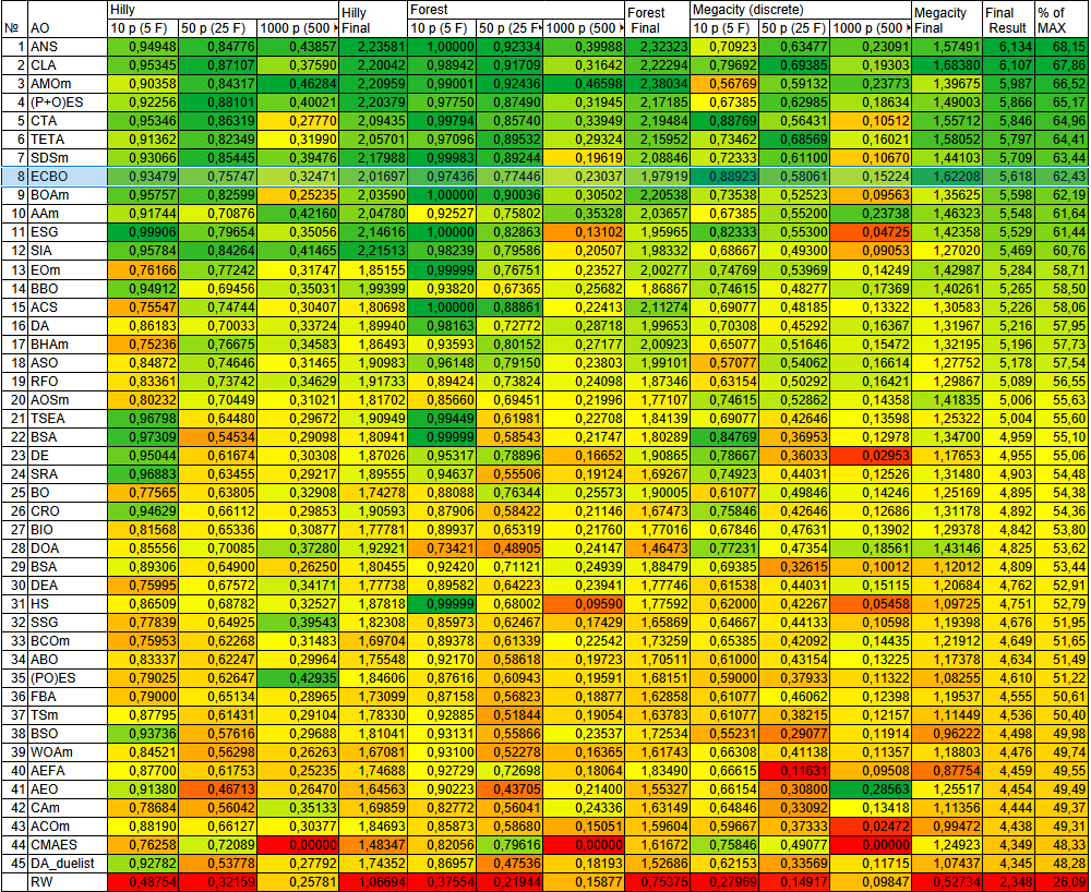
Figure 2. Color coding of algorithms for the corresponding tests

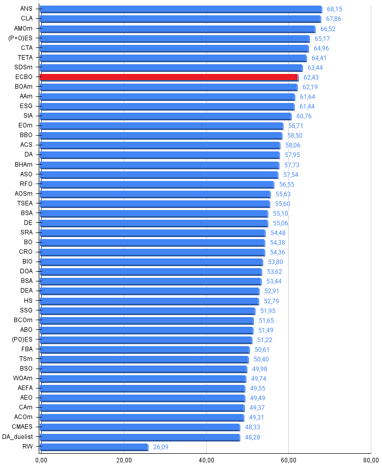
Figure 3. A histogram of the algorithm test results (on a scale from 0 to 100; the higher the score, the better, where 100 is the maximum possible theoretical result; the archive contains a script for calculating the ranking table)

Pros and cons of the ECBO algorithm:

Pros:

1. Strong performance across various types of problems.
2. Few external parameters.
3. Fast.

Cons:

1. A tendency to get stuck on low-dimensional discrete problems.

An archive containing the latest versions of the algorithm codes is attached to the article. The author of this article does not assume responsibility for the absolute accuracy of the descriptions of the canonical algorithms; many of them have been modified to improve their search capabilities. The conclusions and judgments presented in the articles are based on the results of the experiments conducted.

• GitHub: https://github.com/JQSakaJoo/Population-optimization-algorithms-MQL5

Files used in the article

#	Name	Type	Description
1	#C_AO.mqh	Include file	Parent class of population-based optimization algorithms
2	#C_AO_enum.mqh	Include file	Enumeration of population-based optimization algorithms
3	TestFunctions.mqh	Include file	Test function library
4	TestStandFunctions.mqh	Include file	Test bench function library
5	Utilities.mqh	Include file	Utility function library
6	CalculationTestResults.mqh	Include file	Script for calculating results for the comparison table
7	Testing AOs.mq5	Script	Unified test bench for all population-based optimization algorithms
8	Simple use of population optimization algorithms.mq5	Script	Simple example of using population-based optimization algorithms without visualization
9	Test_ECBO.mq5	Script	ECBO test bench