Andean Condor Algorithm (ACA)

Contents

1. Introduction
2. Implementation of the Algorithm
3. Test Results
4. Conclusions

Introduction

In previous articles in this series, a simple hierarchy has emerged among optimization algorithms: at the top are methods that consistently exceed 60% of the total score on standard benchmarks; in the middle — those that stay within the 45–55% range and are suitable for applied problems; at the bottom — algorithms that the authors tested on one or two simple functions and that fail when applied to complex or high-dimensional landscapes. The search for promising algorithms therefore always considers two criteria at once: how readily an algorithm can be reproduced from published sources, and how well it can deliver credible performance figures on a demanding test suite.

Anyone who has ever tuned an Expert Advisor's parameters knows full well why this is necessary. The parameter space is large, and the fitness function landscape is rugged and multimodal. A logical next step is to turn to specialized metaheuristics that can strike a balance between exploration and exploitation of the solution space. But many new algorithms are being released, and most are accompanied by confident claims about their effectiveness, based on tests conducted on just one or two unimodal functions. Algorithms that fall apart on real-world problems can look excellent on the Sphere function — which is why, in this series of articles, each candidate is tested on three benchmarks (Hilly, Forest, Megacity) and at three dimensionalities (10, 50, and 1,000 variables).

Today's candidate is the Andean Condor Algorithm, or ACA, proposed in 2018 by Boris Almonacid and Ricardo Soto for the manufacturing cell formation problem and extended to continuous domains by Almonacid himself in a 2019 paper in PeerJ. The metaphor is the Andean condor's movement pattern when searching for food, which changes from season to season: sometimes wide-ranging flights over the foothills, sometimes local flights around a discovered food source. This is a typical two-phase “exploration/intensification” structure, but with an interesting balancing mechanism: a performance indicator based on the average fitness of the population. Condors with above-average fitness move on to the intensification phase, while the rest continue their exploration.

The main implementation challenge lay in the source publications. The algorithm author's 2019 paper describes only the movement operators and refers readers to the 2018 paper for key details of the balancing mechanism: what exactly the performance indicator does, how each condor's status is calculated from it, and what roles the DP and PC parameters play. Part of this article is therefore devoted to reconstruction: assembling a working version of ACA from the abstract, descriptions of the operators, and a general understanding of metaheuristics. The next step is to compare its behavior with the numerical results that the author did publish for the test problem.

The most interesting discovery came when tuning the population size parameter; more on that below. By the end of the article, the reader will have three things. First, a working C_AO_ACA class in our framework's format, ready to be used in your own optimization tasks. Second, honest results from standard benchmarks, with an analysis of the role of the population size parameter. Third, a methodological lesson on how an algorithm presented by its authors as swarm intelligence is actually structured differently in practice. The article shows how to take this into account when choosing an optimizer for a project.

Implementation of the Algorithm

Biological prototype. The Andean condor (Vultur gryphus) is one of the largest flying birds on the planet, inhabiting the highlands of the Andes from Venezuela to Tierra del Fuego. Its foraging behavior exhibits distinct seasonal patterns: during favorable seasons, the flight radius from the nest is small, and the condor circles known carrion sites and hunts locally; during unfavorable periods, the foraging range expands to hundreds of kilometers, and the bird regularly explores new territories. This alternation between searching the immediate vicinity and long-range exploration forms the basis of the algorithm's metaphor: at any given moment, each individual in the population is either in intensification mode (local refinement) or in exploration mode (broad search), and its mode is determined by a performance indicator — how successful the condor is relative to the rest of the population.

Agent Structure. Each condor stores three blocks of information: a vector of variables $x = (x_1, x_2, \ldots, x_n)$, representing a point in the search space and bounded by the box $[LB, UB]$ for each coordinate; status $S \in \{T, F\}$, indicating the current mode (intensification or exploration); and fitness $f \in \mathbb{R}$ — the value of the objective function at this point.

Population initialization. Initially, each coordinate of each condor is assigned a uniformly distributed random value within its bounds:

$$x_i^{(0)}\sim U(L{B}_i,U{B}_i),i=1,\dots ,n$$

The initial fitness values are calculated once; the statuses can be initialized arbitrarily on the first run — they will be reassigned on the very next iteration.

Performance indicator and status assignment. This is the most interesting part of the algorithm. At each iteration, the population is sorted in descending order of fitness, and the condors at the top of the ranked list are assigned the "intensification" status, while the rest are assigned the "exploration" status. The boundary between groups is defined by the parameter $DP \in [0, 1]$ (Distribution Parameter) — the proportion of the population assigned to the intensification group.

Formally, let $r(i) \in \{0, 1, \ldots, N-1\}$ be the rank of agent $i$ after sorting in descending order (the best has rank 0), and let $N$ be the population size. Then:

$$S_i = \begin{cases} T \text{ (intensification)}, & \text{if } r(i)/N < DP \\ F \text{ (exploration)}, & \text{otherwise} \end{cases}$$​

After that, with a probability of $PC \in [0, 1]$ (Perturbation Coefficient), the status of each agent is inverted. This stochastic adjustment adds a small amount of noise to the strict rank-based division — it occasionally allows the worse agents to switch to intensification mode and the better agents to switch to exploration mode, helping the algorithm avoid premature convergence.

There is an important caveat here. The 2019 paper does not directly describe the performance indicator — the author refers to the 2018 paper. The ranking scheme described above, using the threshold $DP$ and stochastic inversion with probability $PC$, is a reconstruction based on the abstract of the main paper (which mentions “ranking” and “average fitness”) and the general logic of this group of metaheuristics. Alternative interpretations of the mechanism (for example, directly comparing each agent to the average fitness of the population) yield similar but noisier results in the tests.

Example. Suppose a population of 4 condors has fitness values $f = (3, 7, 1, 5)$ in index order, with $DP = 0.5$ and $PC = 0.2$. After sorting in descending order, the ranks are as follows: Agent 1 (f=7) — rank 0, Agent 3 (f=5) — rank 1, Agent 0 (f=3) — rank 2, Agent 2 (f=1) — rank 3. Let's check the condition $r/N < 0.5$: Agents 1 and 3 (normalized ranks 0.0 and 0.25) are assigned the status $T$, while agents 0 and 2 (0.5 and 0.75) receive the status $F$. Then, with a probability of 0.2, each individual’s status may flip—on average, half the population works on intensification and half on exploration in each iteration, but the specific condors in these groups change.

Exploration Operator. Applies to agents with the status $F$. Half of the chosen condor's coordinates are selected at random, with index set $J \subset \{1, \ldots, n\}$, $|J| = \lfloor n/2 \rfloor$. For each $i ∈ J$ the following applies:

$$x_i^{(t+1)} = x_i^{(t)} + \delta_i, \quad \delta_i \sim U(LB_i - x_i^{(t)}, UB_i - x_i^{(t)})$$

If we expand this expression, we get $x_i^{(t+1)} \in [LB_i, UB_i]$, which is equivalent to completely reinitializing this coordinate with a uniform distribution over the entire valid range. The other half of the coordinates remain unchanged. From a geometric perspective, this is a condor’s leap to a random point on a hyperplane orthogonal to the subspace of the remaining coordinates.

Example. A condor in a 4-dimensional problem with $[LB, UB] = [-100, 100]$ is at position $x = (-50, 30, 80, -10)$. Coordinates 1 and 3 are selected at random. For coordinate 1: $\delta_1 \sim U(-100 - 30,\ 100 - 30) = U(-130, 70)$; the new value of $x_1$ lies in $(-100, 100)$. For coordinate 3: $\delta_3 \sim U(-100 + 10,\ 100 + 10) = U(-90, 110)$; the new value of $x_3$ also lies in $(-100, 100)$. The coordinates 0 and 2 remain unchanged. For example, when $\delta_1 = -55$ and $\delta_3 = 75$, the condor's new position is $x_{new} = (-50, -25, 80, 65)$.

Intensification operator. Applied to agents with the status $T$. One coordinate $j \in \{1, \ldots, n\}$ is selected at random, and a perturbation type $\theta \in \{1, 2, 3, 4\}$ is selected at random with equal probabilities. The change is made according to the following rule:

$$x_j^{(t+1)} = x_j^{(t)} + \begin{cases} \alpha, & \theta = 1, \quad \alpha \sim U(0.3 \cdot LB_j,\ 0.3 \cdot UB_j) \\ \beta, & \theta = 2, \quad \beta \sim U(0.1 \cdot LB_j,\ 0.1 \cdot UB_j) \\ \gamma, & \theta = 3, \quad \gamma \sim U(-1, 1) \\ \varepsilon, & \theta = 4, \quad \varepsilon \sim U(-0.05, 0.05) \end{cases}$$​

This provides four perturbation scales within a single operation. For a typical symmetric domain $[-100, 100]$, the operator $\alpha$ produces a jump of up to $\pm 30$ (a large jump, effectively moving into a new region of the search space), $\beta$ — up to $\pm 10$ (a medium jump), $\gamma$ — up to $\pm 1$ (fine-tuning), and $\varepsilon$ — up to $\pm 0.05$ (micro-adjustment). Selecting among them at random with equal probabilities gives the algorithm a built-in multiscale search mechanism: the same population can simultaneously explore distant promising regions using $\alpha$ and refine the optimal value found using $\varepsilon$.

Example. The same condor $x = (-50, 30, 80, -10)$. The result was $j = 2$, $\theta = 3$ (that is, $\gamma$): $\gamma \sim U(-1, 1)$, let $\gamma = 0.4$. The new value is $x_2 = 80 + 0.4 = 80.4$. The other coordinates remain unchanged. If the random selection had instead yielded $\theta = 1$, then $\alpha \sim U(-30, 30)$. Assuming $\alpha = -25$, we would obtain $x_2 = 55$ — a significant jump that moves the condor into a fundamentally different region along this coordinate.

Greedy acceptance. After all condors have generated their new positions, the objective function is computed at all the new points. Acceptance of a new position is greedy: if the fitness of the new position is no worse than that of the old one, the condor remains in the new position; otherwise, it reverts to the position it held before the iteration.

$$x^{(t+1)} = \begin{cases} x_{\text{new}}, & \text{if } f(x_{\text{new}}) \geq f(x^{(t)}) \\ x^{(t)}, & \text{otherwise} \end{cases}$$​

The best position found over the entire search history, $x_B$​, with fitness $f_B$, is also maintained separately and updated whenever a new point improves on the current record. This pair represents the final result of the algorithm's operation.

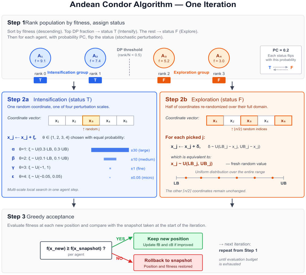
Figure 1. Diagram of the ACA algorithm

The illustration shows the three steps of a single iteration:

Step 1. Ranking of the four condors by fitness, using a dashed line at the DP=0.5 threshold: the top two (A₁, A₂) are blue, indicating intensification; the bottom two (A₃, A₄) are orange, indicating exploration. On the right, a separate block shows the PC mechanism for stochastic status inversion.

Step 2a (blue panel). A coordinate vector is shown with the randomly selected coordinate x₃ highlighted, and the four perturbation scales α/β/γ/ε are visualized as rectangular bands whose sizes convey the differences in orders of magnitude of the amplitude: from a large jump of ±30 to fine-tuning of ±0.05.

Step 2b (orange panel). A vector with three randomly selected coordinates and a scale of the range [LB, UB], with points illustrating the uniform distribution of new values.

Step 3. A greedy check with two outcomes: the green "Keep" branch when $f_{\text{new}} \geq f_{\text{snapshot}}$ and the red "Rollback" branch otherwise, plus a pointer to the next iteration.

The pseudocode for a single iteration of the algorithm looks like this:

Input:  condor population {x_1, ..., x_N} with fitnesses {f_1, ..., f_N}
        parameters DP, PC
        bounds LB, UB

1. Save current population snapshot (for possible roll-back)

2. Ranking:
   Sort condors in descending order of f
   r(i) ← rank of agent i

3. Assigning status:
   for each i = 1..N:
       S_i ← T, if r(i)/N < DP, otherwise F
       with the probability of PC: S_i ← !S_i

4. Moving:
   for each i = 1..N:
       if S_i = T:                                   // intensification
           j  ← random coordinate from {1, ..., n}
           θ  ← random selection from {1, 2, 3, 4}
           ξ  ← sample from distribution α / β / γ / ε by θ
           x_{i,j} ← x_{i,j} + ξ
           
       if S_i = F:                                   // exploration
           J ← random ⌊n/2⌋ coordinates
           for each j from J:
               δ ← U(LB_j − x_{i,j}, UB_j − x_{i,j})
               x_{i,j} ← x_{i,j} + δ

5. Calculate fitnesses of new positions

6. Greedy acceptance:
   for each i = 1..N:
       if f(x_new_i) < f(snapshot_i):
           restore x_i from the snapshot

7. Update global record x_B, f_B

The cycle repeats until the specified limit for objective function evaluations is reached (10,000 in our tests).

Overall, the algorithm is compact: three parameters (population size, $DP$, $PC$), two movement operators, and one greedy acceptance procedure. The agents' states between iterations do not retain any memory of past trajectories — there are no velocities, as in PSO, no pheromones, as in ACO, and no shared long-term memory. In each iteration, every agent solves a local problem: either by fine-tuning a single coordinate or by resetting half of the coordinates for a broader search, based on its rank in the population at that step.

Let's move on to analyzing the implementation. The C_AO_ACA class inherits from our framework’s base class, C_AO, and integrates with the standard optimization method lifecycle by overriding two virtual functions — Moving() and Revision(). The class exposes three parameters: the population size (popSize), the proportion of the population assigned to intensification (DP), and the probability of stochastic status inversion (PC). The default values follow the author's recommendation (popSize = 25, DP = 0.5, PC = 0.2); however, as will be shown in the next section, these settings are far from optimal on complex test functions, and actual peak performance is achieved with a much smaller population.

The constructor sets the algorithm's name string (ao_name), its text description (ao_desc), and a link to the article. In addition, the params[] array is initialized; this array is used to pass the algorithm's parameters to the external test bench and its input parameters. This is the standard procedure for all algorithms in the framework.

The SetParams() method reads the parameter values from params[] back into the class's internal fields and applies safeguards: the DP and PC values are restricted to the range [0, 1]. This validation is needed in case the external tester passes invalid values.

//+------------------------------------------------------------------+
class C_AO_ACA : public C_AO
 {
public:
                    ~C_AO_ACA() {}
                     C_AO_ACA()
   {
    ao_name = "ACA";
    ao_desc = "Andean Condor Algorithm";
    ao_link = "https://www.mql5.com/en/articles/22525";

    popSize = 25;
    DP      = 0.5;
    PC      = 0.2;

    ArrayResize(params, 3);
    params [0].name = "popSize"; params [0].val = popSize;
    params [1].name = "DP";      params [1].val = DP;
    params [2].name = "PC";      params [2].val = PC;
   }

  void               SetParams()
   {
    popSize = (int)params [0].val;
    DP      = params      [1].val;
    PC      = params      [2].val;

    //--- safeguards

    if(DP < 0.0)
      DP = 0.0;
    if(DP > 1.0)
      DP = 1.0;
    if(PC < 0.0)
      PC = 0.0;
    if(PC > 1.0)
      PC = 1.0;
   }

  bool               Init(const double &rangeMinP  [],
                          const double &rangeMaxP  [],
                          const double &rangeStepP [],
                          const int     epochsP = 0);

  void               Moving();
  void               Revision();

  //--- visible parameters
  double             DP;     // proportion of the population assigned to intensification (0..1)
  double             PC;     // probability of status inversion (0..1)

private:
  //--- snapshot for greedy acceptance
  double             snap_c  [];   // [popSize * coords] — a flat buffer
  double             snap_f  [];   // [popSize]

  //--- ranking and statuses
  int                rankIdx [];   // [popSize]
  bool               status  [];   // [popSize] true = intensification

  //--- coordinate selection buffer for exploration (partial Fisher–Yates shuffle)
  int                shuf    [];   // [coords]
 };
//+------------------------------------------------------------------+

The Init() method performs a one-time initialization of the algorithm. First, the base class's StandardInit() method is called — it allocates the array of agents a[], normalizes the input ranges, and initializes the utility fields. Next, the initial population is generated: each coordinate of each condor is assigned a random value uniformly distributed within its valid range [LB_c, UB_c].

These values are stored in the cP[] array, not in c[] — this is a framework convention whereby cP[] stores the agent's previous position, c[] stores the current position, and cB[] stores the best position in the agent's entire history. The very first call to Moving() will transfer the values in cP[] to c[] in order to evaluate the objective function.

Next, the class’s internal buffers are allocated: snap_c (a flat one-dimensional array of size popSize × coords for storing position snapshots), snap_f (an array of snapshot fitness values), rankIdx (a permutation of indices after sorting), status (a Boolean array of agent statuses), and shuf (an auxiliary buffer for the Fisher-Yates partial shuffle when selecting coordinates during exploration).

//+------------------------------------------------------------------+
//|                              Init                                |
//+------------------------------------------------------------------+
bool C_AO_ACA::Init(const double &rangeMinP  [],
                    const double &rangeMaxP  [],
                    const double &rangeStepP [],
                    const int     epochsP = 0)
 {
  if(!StandardInit(rangeMinP, rangeMaxP, rangeStepP))
    return false;

//--- initial random population in cP[] (transferred to c[] on the first call to Moving())
  for(int i = 0; i < popSize; i++)
    for(int c = 0; c < coords; c++)
      a [i].cP [c] = u.RNDfromCI(rangeMin [c], rangeMax [c]);

//--- internal buffers
  ArrayResize(snap_c,  popSize * coords);
  ArrayResize(snap_f,  popSize);
  ArrayResize(rankIdx, popSize);
  ArrayResize(status,  popSize);
  ArrayResize(shuf,    coords);

  return true;
 }
//+------------------------------------------------------------------+

The Moving() method is the workhorse of the algorithm, generating new agent positions in each iteration. The first call is handled differently: if the revision flag has not yet been set (i.e., this is the very start of the process), then c[] is populated from cP[] using the u.SeInDiSp() utility, which simultaneously quantizes the value to the specified step size and adjusts it to respect the bounds. Next, the outer loop will evaluate the initial population, and control will return to Revision().

On the second and all subsequent calls to Moving(), the iteration itself takes place. First of all, the current agent positions and their fitness values are stored in snap_c and snap_f — this snapshot will be needed later for the greedy rollback. The population is then sorted in descending order of fitness using standard bubble sort (when popSize ≤ 25, this is more than sufficient in terms of performance, and there is no point in using a more sophisticated algorithm).

A normalized rank r/N is calculated for each agent, and based on a comparison with the DP threshold, a status is assigned: T for the top DP fraction of the population, and F for the rest. After that, stochastic status inversion is performed — the agent's status is flipped with probability PC, which adds noise to the strict rank-based division.

Once the statuses have been assigned, generation of new agent positions begins. Agents with T status go through the intensification branch: one coordinate j is randomly selected from the coords coordinates, one perturbation type θ is randomly selected from four options (0..3), and the corresponding random increment is added to the value snap_c[i × coords + j] — a sample from U(0.3·LB, 0.3·UB) for θ=0 (α-operator), U(0.1·LB, 0.1·UB) for θ=1 (β), U(−1, 1) for θ=2 (γ), or U(−0.05, 0.05) for θ=3 (ε). The agent's other coordinates remain unchanged.

Agents with F status follow the exploration branch: half of the coordinates are selected without replacement using a partial Fisher–Yates shuffle (we do not need to shuffle the entire shuf array; running the algorithm for the first ⌊n/2⌋ positions is sufficient), and each selected coordinate is fully reinitialized to a random value within its allowed range. In all branches, the result is written to a[i].c and quantized using SeInDiSp().

//+------------------------------------------------------------------+
//|                            Moving                                |
//|                                                                  |
//|  Iteration Structure:                                            |
//|    1. Snapshot of the current population;                        |
//|    2. Ranking by fitness (in descending order—maximization);     |
//|    3. Status assignment: top DP fraction — intensification,      |
//|       remainder — exploration;                                   |
//|    4. PC-based status inversion for each agent;                  |
//|    5. For each agent, generate a new candidate in a[i].c.        |
//+------------------------------------------------------------------+
void C_AO_ACA::Moving()
 {
//--- First pass: cP → c, so that the outer loop evaluates the fitness function
  if(!revision)
   {
    for(int i = 0; i < popSize; i++)
      for(int c = 0; c < coords; c++)
        a [i].c [c] = u.SeInDiSp(a [i].cP [c],
                                 rangeMin  [c],
                                 rangeMax  [c],
                                 rangeStep [c]);
    return;
   }

//--- 1. snapshot
  for(int i = 0; i < popSize; i++)
   {
    for(int c = 0; c < coords; c++)
      snap_c [i * coords + c] = a [i].c [c];
    snap_f [i] = a [i].f;
   }

//--- 2. ranking (in descending order of f)
  for(int i = 0; i < popSize; i++)
    rankIdx [i] = i;

  for(int i = 0; i < popSize - 1; i++)
    for(int j = i + 1; j < popSize; j++)
      if(snap_f [rankIdx [j]] > snap_f [rankIdx [i]])
       {
        int tmp = rankIdx [i];
        rankIdx [i] = rankIdx [j];
        rankIdx [j] = tmp;
       }

//--- 3-4. status + PC-based status inversion
  for(int k = 0; k < popSize; k++)
   {
    int    slot     = rankIdx [k];
    double normRank = (double)k / (double)popSize;
    status [slot]   = (normRank < DP);

    if(u.RNDfromCI(0.0, 1.0) < PC)
      status [slot] = !status [slot];
   }

//--- 5. movement
  for(int i = 0; i < popSize; i++)
   {
    if(status [i])
     {
      //--- INTENSIFICATION: one coordinate, one θ ∈ {1..4}
      int j = (int)u.RNDfromCI(0.0, (double)coords);
      if(j >= coords)
        j = coords - 1;
      if(j < 0)
        j = 0;

      int theta = (int)u.RNDfromCI(0.0, 4.0);
      if(theta > 3)
        theta = 3;
      if(theta < 0)
        theta = 0;

      double xi = 0.0;
      double LB = rangeMin [j];
      double UB = rangeMax [j];

      switch(theta)
       {
        case 0:
          xi = u.RNDfromCI(0.3 * LB, 0.3 * UB);
          break;  // α
        case 1:
          xi = u.RNDfromCI(0.1 * LB, 0.1 * UB);
          break;  // β
        case 2:
          xi = u.RNDfromCI(-1.0, 1.0);
          break;  // γ
        default:
          xi = u.RNDfromCI(-0.05, 0.05);                 // ε
       }

      double v = snap_c [i * coords + j] + xi;
      a [i].c [j] = u.SeInDiSp(v, rangeMin [j], rangeMax [j], rangeStep [j]);
     }
    else
     {
      //--- EXPLORATION: half the coordinates, δ ~ U[LB-x, UB-x]
      int half = coords / 2;
      if(half < 1)
        half = 1;

      // Fisher–Yates partial shuffle: the first half indices are selected at random without replacement
      for(int k = 0; k < coords; k++)
        shuf [k] = k;
      for(int k = 0; k < half; k++)
       {
        int r = k + (int)u.RNDfromCI(0.0, (double)(coords - k));
        if(r >= coords)
          r = coords - 1;
        if(r < k)
          r = k;
        int tmp  = shuf [k];
        shuf [k] = shuf [r];
        shuf [r] = tmp;
       }

      for(int kk = 0; kk < half; kk++)
       {
        int    j     = shuf [kk];
        double x_old = snap_c [i * coords + j];
        double LB    = rangeMin [j];
        double UB    = rangeMax [j];

        double delta = u.RNDfromCI(LB - x_old, UB - x_old);
        double v     = x_old + delta;
        a [i].c [j]  = u.SeInDiSp(v, rangeMin [j], rangeMax [j], rangeStep [j]);
       }
     }
   }
 }
//+------------------------------------------------------------------+

The Revision() method is called by the test harness after the outer loop has evaluated fitness at all new positions. The logic is divided into three parts. The first part updates the personal and global bests: for each agent, if the new fitness is better than its all-time best (a[i].fB), the current agent position and fitness are stored as its new personal best; at the same time, if the new value is better than the global best (the class's fB), that value is updated along with cB. This block is executed before greedy acceptance because we want to capture every new best value, even if the new position is ultimately rejected under the greedy rule.

The second part runs only on the first call to Revision(): if revision == false, the revision flag is set to true, and the method exits, leaving the initial population unchanged — it has already been evaluated and recorded. From the third call to the method onward, the third part — greedy acceptance itself — runs. For each agent, the current fitness a[i].f is compared with the stored value snap_f[i]. If the new fitness is worse than the snapshot value, a rollback is performed: the coordinates are restored from snap_c[i × coords + c], and the fitness is restored from snap_f[i]. If the new fitness is no worse, the changes are accepted as is. This produces a monotonic trajectory for each agent: its fitness never decreases throughout the run.

A few technical notes on the buffer layout. The snapshot snap_c is stored as a flat one-dimensional array of length popSize × coords with row-major indexing: snap_c[i × coords + c] is the value of coordinate c for agent i. In the framework's classes, a wrapper of the form S_AO_Vector containing an array v[] is more commonly used, but in the case of ACA, exactly one such buffer is needed, and creating a separate structure just for it is redundant — a flat array is sufficient, and the index arithmetic fits into a single line. The rankIdx[] buffer is initialized in Moving() with the permutation [0, 1, ..., N−1] and then reordered by descending snap_f[] values. The shuf[] buffer is reused on every iteration within the exploration branch: it contains all coordinate indices from 0 to n−1, and the algorithm partially shuffles it — this is sufficient to obtain ⌊n/2⌋ random indices without repetition in linear time.

//+-----------------------------------------------------------------------------------------+
//|                           Revision                                                      |
//|                                                                                         |
//|  Standard fB/cB update + greedy acceptance: if a new                                    |
//|  fitness worse than the snapshot fitness, restore the agent's coordinates and fitness.  |
//+-----------------------------------------------------------------------------------------+
void C_AO_ACA::Revision()
 {
//--- Update personal bests and the global best
  for(int i = 0; i < popSize; i++)
   {
    if(a [i].f > a [i].fB)
     {
      a [i].fB = a [i].f;
      ArrayCopy(a [i].cB, a [i].c, 0, 0, coords);
     }
    if(a [i].f > fB)
     {
      fB = a [i].f;
      ArrayCopy(cB, a [i].c, 0, 0, coords);
     }
   }

  if(!revision)
   {
    revision = true;
    return;
   }

//--- Greedy acceptance: roll back if fitness worsens
  for(int i = 0; i < popSize; i++)
   {
    if(a [i].f < snap_f [i])
     {
      for(int c = 0; c < coords; c++)
        a [i].c [c] = snap_c [i * coords + c];
      a [i].f = snap_f [i];
     }
   }
 }
//+------------------------------------------------------------------+

Test Results

The author of the article recommends a population size of 25 condors. At this setting, the algorithm achieves an overall score of 41.42%, which is well below the performance threshold of approximately 48%, leaving it outside the rankings.

ACA|Andean Condor Algorithm|25.0|0.5|0.2|
=============================
5 Hilly's; Func runs: 10000; result: 0.8052284199791254
25 Hilly's; Func runs: 10000; result: 0.4537792998744926
500 Hilly's; Func runs: 10000; result: 0.2666586996118199
=============================
5 Forest's; Func runs: 10000; result: 0.6651158271894628
25 Forest's; Func runs: 10000; result: 0.2311713783192359
500 Forest's; Func runs: 10000; result: 0.052890991104486404
=============================
5 Megacity's; Func runs: 10000; result: 0.8093333333333333
25 Megacity's; Func runs: 10000; result: 0.33359999999999995
500 Megacity's; Func runs: 10000; result: 0.11008000000000095
=============================
All score: 3.72786 (41.42%)

However, when the population is drastically reduced, the algorithm's effectiveness increases sharply — the overall score reaches 53.02%, and ACA confidently makes it onto the leaderboard. This inversion is a topic for a separate discussion.

ACA|Andean Condor Algorithm|2.0|0.5|0.2|
=============================
5 Hilly's; Func runs: 10000; result: 0.7844401742263607
25 Hilly's; Func runs: 10000; result: 0.5326017349427434
500 Hilly's; Func runs: 10000; result: 0.33108785513596034
=============================
5 Forest's; Func runs: 10000; result: 0.7907177664055441
25 Forest's; Func runs: 10000; result: 0.44960020772191805
500 Forest's; Func runs: 10000; result: 0.10685016826475134
=============================
5 Megacity's; Func runs: 10000; result: 0.9226666666666667
25 Megacity's; Func runs: 10000; result: 0.6773333333333332
500 Megacity's; Func runs: 10000; result: 0.17613600000000043
=============================
All score: 4.77143 (53.02%)

The anti-cheat test shows trends similar to those of the initial function results in the preceding main test. An honest algorithm.

ACA|Andean Condor Algorithm|2.0|0.5|0.2|
=============================
Composite test: Hilly + Forest + Megacity + Peaks + Skin
Coordinates: 10; Epochs: 10000; Repeats: 10
=============================
Run 1/10: 0.8549286580531176
Run 2/10: 0.7878587377860654
Run 3/10: 0.7878587377860654
Run 4/10: 0.7878587377860654
Run 5/10: 0.7878587377860654
Run 6/10: 0.7878587377860654
Run 7/10: 0.7878587377860654
Run 8/10: 0.786583205099778
Run 9/10: 0.786583205099778
Run 10/10: 0.786583205099778
=============================
Average result: 0.7941830700 (79.42%)
=============================

The following figures illustrate how the ACA algorithm works on test functions as well as on the functions included in the package.

ACA on the Hilly test function

ACA on the Forest test function

ACA on the Megacity test function

ACA on the Ackley function

ACA on the GoldsteinPrice function

Based on the test results, the ACA algorithm ranks 37th.

cc	AO	Description	Hilly			Hilly Final	Forest			Forest Final	Megacity (discrete)			Megacity Final	Final Result	% of MAX
			10 p (5 F)	50 p (25 F)	1,000 p (500 F)		10 p (5 F)	50 p (25 F)	1,000 p (500 F)		10 p (5 F)	50 p (25 F)	1,000 p (500 F)
1	ANS	across neighbourhood search	1.00000	0.88228	0.40138	2.28366	1.00000	0.95281	0.28092	2.23373	0.94667	0.85733	0.22389	2.02789	6.545	72.72
2	AMOm	animal migration optimization M	0.91624	0.83603	0.46790	2.22017	0.98482	0.92010	0.36391	2.26883	0.91733	0.81707	0.25177	1.98617	6.475	71.94
3	CLA	code lock algorithm (joo)	0.95139	0.86199	0.37879	2.19217	0.99349	0.93500	0.26497	2.19346	0.93600	0.84267	0.24060	2.01927	6.405	71.17
4	(P+O)ES	(P+O) evolution strategies	0.86571	0.89539	0.39740	2.15850	0.97761	0.89820	0.26878	2.14459	0.92133	0.80240	0.23952	1.96325	6.266	69.62
5	SDSm	stochastic diffusion search M	0.95195	0.84944	0.36249	2.16388	0.98061	0.88457	0.22112	2.08630	0.92267	0.79013	0.21380	1.92660	6.177	68.63
6	AAm	archery algorithm M	0.84685	0.73320	0.42590	2.00595	0.96709	0.77837	0.27789	2.02335	0.86133	0.77707	0.28712	1.92552	5.955	66.17
7	SIA	simulated isotropic annealing (joo)	0.93543	0.86504	0.38483	2.18530	0.94069	0.80609	0.23835	1.98513	0.86400	0.66160	0.19536	1.72096	5.891	65.46
8	TETA	time evolution travel algorithm (joo)	0.91452	0.86369	0.25579	2.03400	0.99654	0.91291	0.14394	2.05339	0.85467	0.82213	0.10443	1.78123	5.869	65.21
9	ESG	evolution of social groups (joo)	0.98111	0.79857	0.31167	2.09135	0.98954	0.82270	0.15032	1.96256	0.92133	0.73440	0.15315	1.80888	5.863	65.14
10	CTA	comet tail algorithm (joo)	0.92435	0.86786	0.27838	2.07059	0.99039	0.84571	0.19448	2.03058	0.95467	0.69680	0.11008	1.76155	5.863	65.14
11	ECBO	enhanced colliding bodies optimization	0.94024	0.72363	0.32356	1.98743	0.99477	0.80291	0.13056	1.92824	0.87600	0.70160	0.17433	1.75193	5.668	62.98
12	DA	dialectical algorithm	0.93117	0.75400	0.26205	1.94722	0.98925	0.81375	0.08662	1.88962	0.92667	0.68107	0.11315	1.72089	5.558	61.76
13	BBO	biogeography-based optimization	0.95876	0.70609	0.35752	2.02237	0.92981	0.70660	0.16970	1.80611	0.87467	0.63013	0.20813	1.71293	5.541	61.57
14	BHAm	black hole algorithm M	0.79558	0.76207	0.34682	1.90447	0.99836	0.75798	0.13826	1.89460	0.85067	0.64427	0.17020	1.66514	5.464	60.71
15	HS	harmony search	0.91420	0.69049	0.29924	1.90393	0.97627	0.73373	0.14193	1.85193	0.91733	0.62720	0.15364	1.69817	5.454	60.60
16	RFO	royal flush optimization (joo)	0.80989	0.74481	0.34546	1.90016	0.95251	0.77926	0.15185	1.88362	0.80400	0.66427	0.19071	1.65898	5.443	60.48
17	BOAm	billiards optimization algorithm M	0.76177	0.72421	0.25275	1.73873	0.90890	0.81960	0.28853	2.01703	0.83733	0.74613	0.09763	1.68109	5.437	60.41
18	ASO	anarchy society optimization	0.73070	0.73713	0.31195	1.77978	0.99732	0.87700	0.17619	2.05051	0.72000	0.68773	0.18988	1.59761	5.428	60.31
19	EOm	extremal optimization_M	0.76527	0.75205	0.31908	1.83640	0.99999	0.76426	0.12437	1.88862	0.84133	0.64133	0.15247	1.63513	5.360	59.56
20	ACS	artificial cooperative search	0.75545	0.77162	0.31653	1.84360	1.00000	0.80488	0.10705	1.91193	0.76933	0.60800	0.14157	1.51890	5.274	58.60
21	SSG	saplings sowing and growing	0.75436	0.63206	0.35935	1.74577	0.91907	0.69694	0.19755	1.81356	0.81867	0.60533	0.21347	1.63747	5.197	57.74
22	AOSm	atomic orbital search M	0.76184	0.68435	0.31344	1.75963	0.90015	0.80044	0.11501	1.81560	0.82800	0.63280	0.15696	1.61776	5.193	57.70
23	TSEA	turtle shell evolution algorithm (joo)	0.95809	0.64852	0.29571	1.90232	0.99522	0.58104	0.10542	1.68168	0.92133	0.52160	0.14567	1.58860	5.173	57.48
24	DE	differential evolution	0.96398	0.62346	0.26089	1.84833	0.98482	0.77018	0.11459	1.86959	0.93067	0.36213	0.11000	1.40280	5.121	56.90
25	BIO	blood inheritance optimization (joo)	0.72580	0.66522	0.31228	1.70330	0.99995	0.68125	0.11540	1.79660	0.85467	0.59333	0.15364	1.60164	5.102	56.69
26	(PO)ES	(PO) evolution strategies	0.73972	0.58190	0.38896	1.71058	0.91199	0.59975	0.21262	1.72436	0.82400	0.56240	0.23432	1.62072	5.056	56.18
27	BO	bonobo optimizer	0.75555	0.64366	0.32657	1.72578	0.94332	0.70442	0.13999	1.78773	0.73467	0.61440	0.16728	1.51635	5.030	55.89
28	SRA	successful restaurateur algorithm (joo)	0.89010	0.63359	0.29115	1.81484	0.96634	0.55285	0.08914	1.60833	0.89333	0.52800	0.13911	1.56044	4.984	55.38
29	CRO	chemical reaction optimisation	0.91281	0.65681	0.29866	1.86828	0.90513	0.56020	0.10939	1.57472	0.82800	0.50133	0.14149	1.47082	4.914	54.60
30	BCOm	bacterial chemotaxis optimization M	0.82589	0.61733	0.31584	1.75906	0.95296	0.63718	0.11984	1.70998	0.76533	0.51653	0.15800	1.43986	4.909	54.54
31	DOA	dream optimization algorithm	0.78522	0.78121	0.36036	1.92679	0.61584	0.42117	0.12254	1.15955	0.86667	0.72587	0.21127	1.80381	4.890	54.33
32	ABO	african buffalo optimization	0.92295	0.62528	0.29885	1.84708	0.92992	0.57468	0.09372	1.59832	0.73333	0.51333	0.14324	1.38990	4.835	53.72
33	BSA	bird swarm algorithm	0.94432	0.67941	0.26401	1.88774	0.91649	0.65619	0.12054	1.69322	0.80933	0.33547	0.10652	1.25132	4.832	53.69
34	TSm	tabu search M	0.87806	0.61040	0.28993	1.77839	0.98116	0.52165	0.08544	1.58825	0.82667	0.49547	0.13552	1.45766	4.824	53.60
35	BSA	backtracking search algorithm	0.87128	0.53190	0.28675	1.68993	0.92408	0.51602	0.09153	1.53163	0.96000	0.47253	0.13760	1.57013	4.792	53.24
36	WOAm	whale optimization algorithm M	0.93893	0.59477	0.26695	1.80065	0.98036	0.53873	0.07112	1.59021	0.78667	0.47600	0.11892	1.38159	4.772	53.02
37	ACA	andean_condor_algorithm	0.78444	0.53260	0.33108	1.64812	0.79071	0.44960	0.10685	1.34716	0.92266	0.67733	0.17613	1.77612	4.771	53.02
38	CSO	competitive swarm optimizer	0.85151	0.60786	0.29896	1.75833	0.84085	0.58491	0.11974	1.54550	0.80000	0.48560	0.14184	1.42744	4.731	52.57
39	FBA	fractal-based algorithm	0.69419	0.64267	0.28955	1.62641	0.99812	0.54905	0.08705	1.63422	0.76133	0.51253	0.13689	1.41075	4.671	51.90
40	ECOi	eco-inspired evolutionary algorithm	0.78817	0.54402	0.29360	1.62579	0.88996	0.46592	0.09747	1.45335	0.78533	0.45173	0.14295	1.38001	4.459	49.54
41	BSO	brain storm optimization	0.92207	0.57625	0.29732	1.79564	0.80764	0.42508	0.09448	1.32720	0.77200	0.36533	0.13065	1.26798	4.391	48.79
42	CAm	camel algorithm M	0.71534	0.56917	0.35985	1.64436	0.84094	0.47174	0.10850	1.42118	0.70400	0.41947	0.19563	1.31910	4.385	48.72
43	ACOm	ant colony optimization_M	0.71885	0.48410	0.30990	1.51285	0.75792	0.48639	0.11871	1.36302	0.83600	0.48667	0.16148	1.48415	4.360	48.44
44	BSO	brain storm optimization	0.91331	0.55813	0.29705	1.76849	0.85329	0.44038	0.09447	1.38814	0.72267	0.32880	0.13325	1.18472	4.341	48.23
45	AEFA	artificial electric field algorithm	0.88798	0.65769	0.25276	1.79843	0.95550	0.63602	0.03946	1.63098	0.60800	0.16000	0.09845	0.86645	4.296	47.73
	RW	random walk	0.49970	0.32333	0.25791	1.08094	0.30754	0.11470	0.04400	0.46624	0.36133	0.17013	0.10244	0.63390	2.181	24.23

Conclusions

In the study, the Andean Condor Algorithm proved to be an algorithm with its own distinct characteristics and strengths. When configured according to the author's recommendations (population size 25, DP = 0.5, PC = 0.2), the overall score was 41.42%. However, when the population is reduced to two condors, the algorithm's score rises to 53.02%, placing it firmly in the top 45. On an extended composite of five functions in 10 dimensions, it reaches 79.42%, which dispels suspicions of overfitting to the three standard functions and confirms its strength in low-dimensional problems.

The algorithm's performance on the Megacity function is particularly noteworthy. This is a discrete, stepped landscape with flat plateaus between levels, and many metaheuristics struggle with this type of geometry; on the plateaus, there is simply nothing to latch onto, and the direction of improvement cannot be determined. ACA has a structural advantage here. A multi-scale intensification operator with four perturbation categories allows the algorithm to search for the right “tile” using large α- and β-jumps while refining the position within it using small γ- and ε-steps, and greedy acceptance naturally accommodates stepwise improvements in the objective function.

The internal structure of ACA has several notable features. First, it is a compact algorithm with a minimal set of parameters — three in total, two of which (DP and PC) determine the balance between intensification and exploration, and the third specifies the population size. Second, the exploration operator reinitializes half of the coordinates with values drawn completely at random from their full ranges — an uncommon technique among metaheuristics: most exploration algorithms make gradual shifts with a radius that decreases over time, whereas here the selected axes undergo a complete reset. This results in a stochastic combination of local refinements and fundamentally nonlocal jumps, with the balance between them automatically adjusted through fitness-based ranking. Third, the absence of internal memory between iterations makes the algorithm easy to implement, memory-efficient, and predictable in its behavior — each iteration is self-contained and does not depend on a long history.

Reducing the population size improves the algorithm's performance; the optimal number is two to four agents. There is a clear explanation for this under a fixed computational budget: with 10,000 fitness function evaluations, a smaller population means more iterations per agent and, consequently, more updates to each coordinate in intensification mode. Therefore, the author's recommendation of 25 condors turns out not to be optimal for our test set.

An important caveat applies to all results. Since the performance indicator mechanism was reconstructed from the abstract of the main paper published in 2018, some implementation details are a matter of interpretation: the exact semantics of the DP and PC parameters, the ranking scheme, and the method for calculating the threshold. In testing, alternative interpretations of these elements yield similar results, but with different characteristics. This means that the numbers given here characterize our reconstructed implementation of ACA, not the authors' original implementation, which may behave slightly differently in certain respects.

From a practical standpoint, it makes sense for a trader to consider ACA primarily for problems where the objective function has a discrete or stepwise response. This is especially true for problems with up to 20–30 parameters. Here, the algorithm will operate predictably, quickly, and with minimal manual configuration. For high-dimensional problems with a smooth, continuous landscape, ACA is a less natural fit, and it is worth comparing it with algorithms designed for such conditions.

In short: ACA is a compact, multi-scale optimizer with two unusual features (complete reinitialization of half the coordinates during exploration and stochastic selection of amplitude from four categories during intensification), which performs particularly well on low-dimensional discrete and stepwise functions, requires minimal tuning, and is suitable for relevant applied problems.

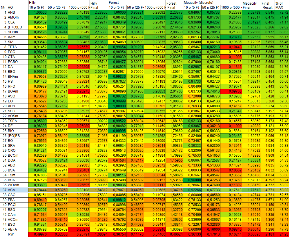
Figure 2. Color coding of algorithms by test

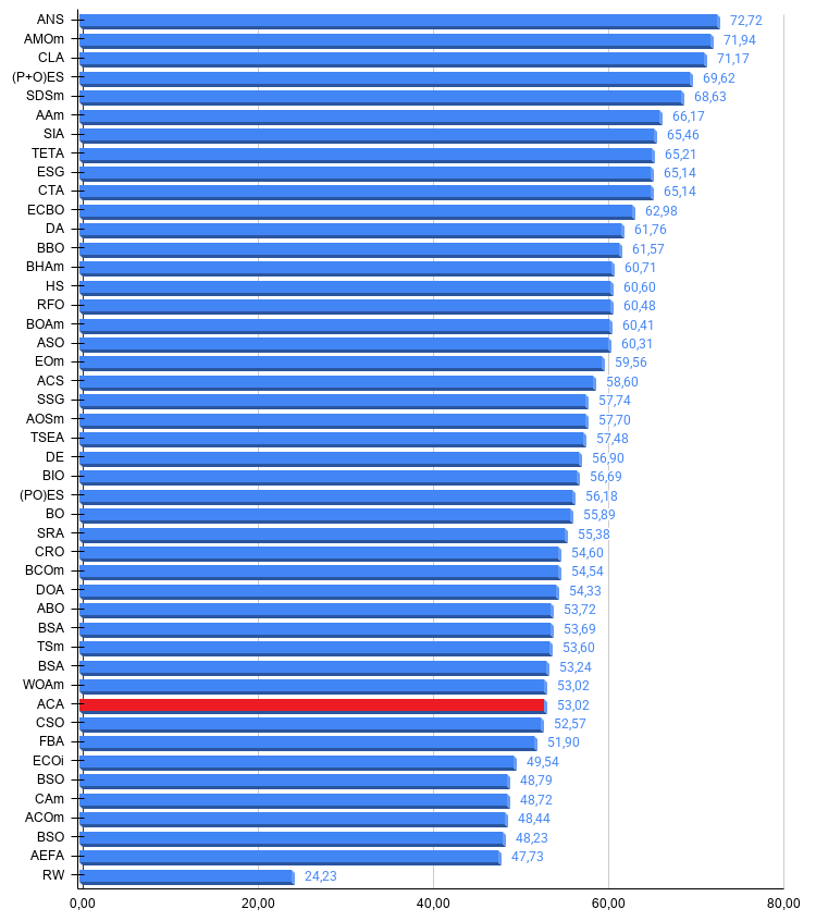
Figure 3. A histogram of the algorithm test results (on a scale from 0 to 100; the higher the score, the better, where 100 is the maximum possible theoretical result); the archive contains a script for calculating the ranking table

Pros and Cons of the Algorithm

Pros:

1. A small number of external parameters.
2. Strong performance on the discrete Megacity test function.

Cons:

1. Tendency to become stuck.

An archive containing the latest versions of the algorithm source code is attached to the article. The author of this article does not guarantee the absolute accuracy of the descriptions of canonical algorithms; many of them have been modified to improve their search capabilities. The conclusions and assessments presented in the articles are based on the results of the experiments conducted.

• GitHub: https://github.com/JQSakaJoo/Population-optimization-algorithms-MQL5

Software used in this article

#	Name	Type	Description
1	#C_AO.mqh	Include file	Parent class of population-based optimization algorithms
2	#C_AO_enum.mqh	Include file	Enumeration of population-based optimization algorithms
3	TestFunctions.mqh	Include file	Test function library
4	TestStandFunctions.mqh	Include file	Test bench function library
5	TestStand3D.mqh	Include file	3D visualization panel for a test bench
6	Utilities.mqh	Include file	Utility functions library
7	CalculationTestResults.mqh	Include file	Script for calculating results for a comparison table
8	Test_AO_All.mq5	Script	Unified test bench for all population-based optimization algorithms
9	Test_AO_AntiCheat	Script	Test for cheating by optimization algorithms
10	Simple use of population optimization algorithms.mq5	Script	Simple example of using population-based optimization algorithms without visualization
11	Test_AO_ACA.mq5	Script	ACA test bench