

James-Stein Shrinkage: Estimating Many Numbers at Once, and Testing What It Buys
 121
 0

Contents
- Introduction
- What shrinkage does to a set of estimates
- The estimator, and where the theorem starts
- Shrinking toward a fixed target
- Shrinking toward the grand mean, and why k must reach four
- The positive part, and the two degenerate inputs
- Unequal variances: the form that can change a ranking
- Estimating the between-group variance
- A weight for every coordinate
- Win rates, and why a proportion needs a transform
- What shrinkage costs
- Verifying the library
- On real prices: choosing a Donchian lookback
- Reading it on a chart: the hour-of-day table
- Conclusion
Introduction
Every trading workflow produces a table of numbers measured side by side. An optimizer reports the average return of eight Donchian lookbacks. A session study reports the mean return of twenty-four hours of the day. A portfolio review reports the win rate of a dozen symbols. The habit is always the same: sort the table and keep the top row.
That habit has a known failure mode. Each row is a mean estimated from a finite sample, so each carries its own noise, and the largest value in a noisy list is the one whose noise happened to point up. Take the same measurement again on fresh data and the winner regresses. The effect is not subtle: it is the reason an optimizer's best parameter set so rarely repeats out of sample.
In 1961 Willard James and Charles Stein published a result that reads as a paradox on first contact. If you estimate three or more means at the same time, the vector of sample means is not admissible under total squared error. Pull every estimate a little toward a common center and the expected total squared error falls, for every true configuration of the means. The guarantee is an average over repeated samples, not a promise about any single data set: on one draw the shrunk vector can land further from the truth than the raw one, and the article measures how often. The coordinates need not even be related, which is the part that sounds absurd and is nevertheless a theorem.
This article builds that estimator in MQL5, together with the empirical Bayes generalization that handles what an actual trading table always presents: coordinates measured with different precision. It then does the part most treatments skip. The theorem concerns estimation, whereas traders care about selection; these are different questions. The study here asks both on the same data, and the answers come back different enough that the distinction has to be taken seriously.
What shrinkage does to a set of estimates
Before any code, here is the result the library is built to reproduce. Ten true means are set a known distance apart. Each is observed once with unit noise. Two estimators are compared on the same draw: the raw observations and the observations shrunk toward their grand mean. The experiment repeats 20,000 times at each separation, and scoring both on the same draw cancels the noise they share and sharply narrows the error bar on the difference. It does not remove sampling noise altogether, so the curve below is a Monte Carlo estimate of the risk rather than the risk itself.
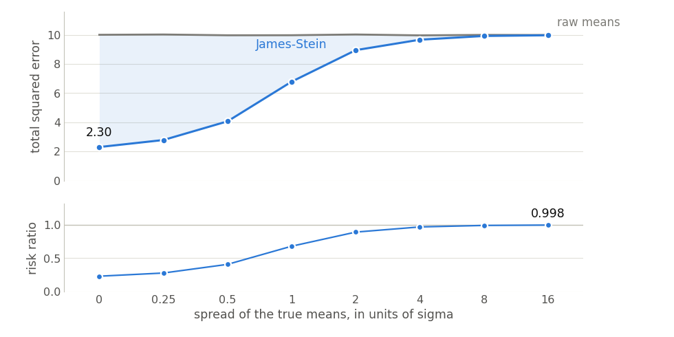
Fig. 1. The raw risk sits flat at ten while the James-Stein risk starts near two and climbs toward it, staying below it at every separation measured
The upper panel is the measurement, and the shaded band between the two curves is the whole result. Raw risk is flat at ten, which is k times sigma squared, exactly what theory says the sample mean delivers. The James-Stein curve begins at 2.30 when all ten truths coincide and rises toward ten as they separate, so the band is widest on the left and closes on the right. The strip underneath is the same thing as a ratio, running from 0.230 at zero separation to 0.998 at sixteen sigma: across the eight separations measured it approaches one from below without reaching it.
Two things in that picture are worth holding on to. The gain is largest exactly when the coordinates really are alike, which is the case a trader faces when eight lookbacks of one strategy are all mediocre in the same way. And the saving never turns into a penalty: the expected risk of the shrunk vector is at or below the raw risk at every true configuration, which is what makes this a theorem rather than a heuristic that works on friendly data. The figure adds one practical check: it validates the implementation on a finite grid of separations. Eight separations cannot establish a theorem, and with the theorem's assumptions in force it cannot overturn one either. A point on the wrong side would say that the implementation is wrong, that an assumption has been broken, or that the replications were too few to resolve the difference.
That is what this article delivers. The rest explains how, and then asks what happens when the same estimator meets real prices.
The estimator, and where the theorem starts
The whole library lives in one header, JamesStein.mqh, with no class and no state. Drop it in MQL5\Include\JamesStein\, write #include <JamesStein\JamesStein.mqh> at the top of your script, expert or indicator, and there is nothing else to set up. Each entry point takes an array, writes a shrunk array, and fills a diagnostics struct. That struct matters more than it looks: a caller who cannot see how much the data was trusted cannot tell a strong pull from a weak one.
//+------------------------------------------------------------------+
//| JSResult                                                         |
//|                                                                  |
//|  What the estimator did, not only what it returned. The factor   |
//|  and tau2 are the whole story of how much the data was trusted,  |
//|  so they are reported rather than hidden inside the call.        |
//+------------------------------------------------------------------+
struct JSResult
  {
   int               k;         // number of coordinates estimated together
   double            dof;       // (k-2), (k-3) or (k-1), whichever the method used
   double            target;    // the point everything was pulled toward
   double            tau2;      // between-coordinate variance, 0 if not fitted
   double            factor;    // the common B, or its mean when B is per-coordinate
   bool              clamped;   // B reached its ceiling of 1
   bool              dominates; // k is large enough for the theorem to apply
   bool              valid;     // inputs were usable
   string            note;      // anything worth reading, empty when there is none
  };
The two fields to watch are factor and dominates. The factor is B, the fraction of the distance from each observation to the center that gets removed; B near zero leaves the data almost untouched, B equal to one collapses everything onto the center. That reading is exact only for the two equal-variance forms below, which apply one common B to every coordinate. The empirical Bayes form weights each coordinate separately, and factor then holds the average of those weights rather than a number applied to any one of them, so the pull on a single coordinate has to be read from the per-coordinate factor array the call fills, which is the array the study and the indicator receive as bf. The dominates flag says whether the configuration is one the theorem covers, and it is false more often than a casual reading of the literature suggests.
Shrinking toward a fixed target
The original form pulls toward a point chosen in advance, zero for example, or a benchmark return the desk already believes in. Write x for the vector of observations, sigma2 for the common known variance of each, and t for the target. Then
B = (k - 2) * sigma2 / sum((x_i - t)^2)

shrunk_i = t + (1 - B) * (x_i - t)
The denominator is the whole mechanism in one term. When the observations sit far from the target their spread is large, B is small, and almost nothing is removed. When they huddle near the target the spread is small, B is large, and most of the apparent structure is treated as noise and deleted.
//+------------------------------------------------------------------+
//| Shrink toward a fixed, externally chosen target                  |
//|                                                                  |
//|  The original 1961 estimator. Because the target costs no        |
//|  degree of freedom the constant is (k-2) and the theorem holds   |
//|  from k = 3 upward, for a variance that is known and positive.   |
//+------------------------------------------------------------------+
bool JSShrinkToTarget(const double &x[], const double sigma2,
                      const double target, double &shrunk[], JSResult &res)
  {
   JSClearResult(res);
   int k = ArraySize(x);
   res.k      = k;
   res.target = target;

   if(k < 3)
     {
      res.note = "k must be at least 3";
      return(false);
     }

//--- the dominance result is stated for a known positive variance, so
//--- the noiseless case is refused rather than answered
   if(!(sigma2 > 0.0) || !MathIsValidNumber(sigma2))
     {
      res.note = "sigma2 must be finite and strictly positive";
      return(false);
     }
   if(!MathIsValidNumber(target))
     {
      res.note = "target must be finite";
      return(false);
     }

//--- a single unusable observation reaches every output through the
//--- shared sum, so it is named here rather than carried forward
   for(int i = 0; i < k; i++)
      if(!MathIsValidNumber(x[i]))
        {
         res.note = "every observation must be finite";
         return(false);
        }

   ArrayResize(shrunk, k);
   res.dof       = k - 2;
   res.dominates = true;

   double ss = JSSumSquaredDeviation(x, target);

//--- every observation already sits on the target, so B has no
//--- finite limit and the positive part reports it at its ceiling
   if(ss <= 0.0)
     {
      res.factor  = 1.0;
      res.clamped = true;
      res.note    = "zero spread, so B is reported at its ceiling of 1";
      for(int i = 0; i < k; i++)
         shrunk[i] = x[i];
      res.valid = true;
      return(true);
     }

   double b = res.dof * sigma2 / ss;
   if(b > 1.0)
     {
      b = 1.0;
      res.clamped = true;
     }
   res.factor = b;

   for(int i = 0; i < k; i++)
      shrunk[i] = target + (1.0 - b) * (x[i] - target);

   res.valid = true;
   return(true);
  }
The constant is (k - 2) because the target cost nothing to obtain: it was supplied from outside and the data were not consulted to find it. That is why three coordinates are already enough here, and the function sets dominates to true as soon as k reaches three, for the known positive variance the theorem assumes and the guard above it requires.
Shrinking toward the grand mean, and why k must reach four
In practice nobody knows the right target, so the natural move is to use the average of the observations themselves. That version is the one a trading table wants, and it carries a cost that is easy to miss.
//+------------------------------------------------------------------+
//| Shrink toward the grand mean of the observations themselves      |
//|                                                                  |
//|  Estimating the target from the same data costs one degree of    |
//|  freedom, so the constant drops to (k-3). At k = 3 that constant |
//|  is zero, the estimator returns its input untouched, and         |
//|  dominance only begins at k = 4.                                 |
//+------------------------------------------------------------------+
bool JSShrinkToGrandMean(const double &x[], const double sigma2,
                         double &shrunk[], JSResult &res)
  {
   JSClearResult(res);
   int k = ArraySize(x);
   res.k = k;

   if(k < 3)
     {
      res.note = "k must be at least 3";
      return(false);
     }

//--- the dominance result is stated for a known positive variance, so
//--- the noiseless case is refused rather than answered
   if(!(sigma2 > 0.0) || !MathIsValidNumber(sigma2))
     {
      res.note = "sigma2 must be finite and strictly positive";
      return(false);
     }

//--- the center is built from every observation, so one unusable
//--- entry would reach all of them through the mean
   for(int i = 0; i < k; i++)
      if(!MathIsValidNumber(x[i]))
        {
         res.note = "every observation must be finite";
         return(false);
        }

   ArrayResize(shrunk, k);
   double gm = JSMean(x);
   res.target    = gm;
   res.dof       = k - 3;
   res.dominates = (k >= 4);
   if(!res.dominates)
      res.note = "k = 3 zeroes the (k-3) constant; result equals the input";

   double ss = JSSumSquaredDeviation(x, gm);

//--- identical observations leave zero spread, so B clamps
   if(ss <= 0.0)
     {
      res.factor  = 1.0;
      res.clamped = true;
      res.note    = (res.note == "" ? "" : res.note + "; ") +
                    "zero spread, so B is reported at its ceiling of 1";
      for(int i = 0; i < k; i++)
         shrunk[i] = x[i];
      res.valid = true;
      return(true);
     }

   double b = res.dof * sigma2 / ss;
   if(b > 1.0)
     {
      b = 1.0;
      res.clamped = true;
     }
   res.factor = b;

   for(int i = 0; i < k; i++)
      shrunk[i] = gm + (1.0 - b) * (x[i] - gm);

   res.valid = true;
   return(true);
  }
The constant drops from (k - 2) to (k - 3). Estimating the center from the same numbers that are about to be shrunk spends one degree of freedom, and the estimator has to pay for it. At k equal to three the constant is exactly zero, B is zero, and the function returns its input untouched. That is not a rounding artifact. Three numbers minus their own mean still leave two degrees of freedom, so their spread is perfectly measurable, and what vanishes is the constant rather than the information. The estimator declines to shrink because the guarantee has run out. That covers any three numbers that differ; three identical numbers reach a different branch, which the next section takes up, and there the factor is not zero.
Dominance therefore begins at k equal to four for this form, not at three. That is worth stating loudly: a harness written around the k greater than or equal to three rule will sit at k equal to three, see that shrinkage does nothing, and report a defect that does not exist.
The positive part, and the two degenerate inputs
Nothing in the formula stops B from exceeding one. When the noise is large relative to the spread the raw factor overshoots, and a literal application would push every observation past the center and out the other side. The fix, due to Baranchik, is the positive part: clamp B at one, which collapses the vector onto the center and stops there. Both functions record it in clamped, so a caller can tell a vector pulled all the way to its center from one merely pulled hard.
The other edge is a vector whose observations are all identical. The sum of squared deviations is then zero, and the factor would be a division by zero. The code tests for it before dividing and hands the input straight back. The values are right either way: every observation already sits on the center and no pull could move it. The diagnostic follows the limit rather than the arithmetic. As the spread falls to zero B runs to infinity, so the positive part reports it at the ceiling: the factor comes back as 1.0 with clamped set, and the note names the zero spread as the reason.
On the factor alone that reads as a vector collapsed entirely onto its center, when what happened is that there was no distance to collapse. The note is what separates the two, and it is why the struct carries one. This branch is tested before any degree of freedom is spent, which settles the k equal to three case left open above: three identical numbers take this path rather than the (k - 3) path, so the output is the input and the factor reads 1.0 rather than 0.
Unequal variances: the form that can change a ranking
Everything so far assumes one common, known variance. A real table never looks like that. In the study below, a Donchian lookback of ten averages 64.2 trades per in-sample window while a lookback of a hundred averages 8.1, and the study measures what that does to their error bars rather than inferring it: the mean standard error runs from 6.983e-04 to 4.800e-03, a factor of 6.87. Two effects compound to widen the error bars. The trade count falls by a factor of 7.9, which alone would widen the error bar by its square root, and the per-trade spread also climbs, from 5.526e-03 to 1.323e-02, because a longer channel holds a position longer. An hour-of-day table has the same problem for a different reason: the hours differ in bar count and in volatility. Unequal variances matter for anyone hoping to use this for selection.
Here is why. With one common B, every coordinate moves by the same fraction of its distance to a common center. That map is monotone: if x_i was above x_j before, it is above it after. The plain equal-variance estimators in this header can never reorder a ranking. They change the numbers and leave the argmax exactly where it was. That claim is about these two functions, which share one factor and one target across every coordinate, and not about equal-variance procedures in general: a rule shrinking different coordinates toward different targets would reorder even with a single factor. Only a per-coordinate weight lets a steadier rival overtake a lucky leader, and that requires the empirical Bayes form.
Estimating the between-group variance
The per-coordinate weight is sigma2_i / (tau2 + sigma2_i), where tau2 is the variance of the true means around their common center. A coordinate whose own measurement error is large compared to the real spread gets pulled hard; one measured precisely keeps its value. So tau2 has to be estimated, and the library uses the moment estimator of DerSimonian and Laird, which is closed form and needs no iteration.
//+------------------------------------------------------------------+
//| DerSimonian-Laird moment estimate of the between-group variance  |
//|                                                                  |
//|  Q measures how much more the observations scatter than their    |
//|  own noise explains. Whatever is left over after subtracting     |
//|  (k-1) is attributed to real spread, and the moment estimate is  |
//|  truncated at zero, which makes a zero a floor and not a fact.   |
//+------------------------------------------------------------------+
double JSEstimateTau2DL(const double &x[], const double &sigma2[])
  {
   int k = ArraySize(x);
   if(k < 2 || ArraySize(sigma2) != k)
      return(0.0);

//--- the weights are reciprocals, so a single unusable variance would
//--- poison every sum below rather than only its own term
   for(int i = 0; i < k; i++)
      if(!(sigma2[i] > 0.0) || !MathIsValidNumber(sigma2[i]))
         return(0.0);

   double sw = 0.0, sw2 = 0.0, swx = 0.0;
   for(int i = 0; i < k; i++)
     {
      double w = 1.0 / sigma2[i];
      sw  += w;
      sw2 += w * w;
      swx += w * x[i];
     }
   if(sw <= 0.0)
      return(0.0);

   double muFixed = swx / sw;

   double q = 0.0;
   for(int i = 0; i < k; i++)
     {
      double w = 1.0 / sigma2[i];
      double d = x[i] - muFixed;
      q += w * d * d;
     }

   double c = sw - sw2 / sw;
   if(c <= 0.0)
      return(0.0);

   double tau2 = (q - (k - 1)) / c;
   if(tau2 < 0.0 || !MathIsValidNumber(tau2))
      tau2 = 0.0;
   return(tau2);
  }
Q is a weighted sum of squared deviations from the precision-weighted mean. If the coordinates differed only by their own measurement noise, Q would average (k - 1). Whatever exceeds that is attributed to real spread, divided by the scaling constant c to put it back on the variance scale. A negative leftover is not a variance, so the moment estimate is truncated at zero. Read that zero carefully: it records that this estimator found no positive between-group variance, not that none exists. A small k or too little data will produce the same zero from a table whose true means really do differ.
Note the loop that rejects any non-positive or non-finite variance before anything is summed. The weights are reciprocals, so a single unusable entry would not merely spoil its own term, it would poison every sum in the function.
A weight for every coordinate
//+------------------------------------------------------------------+
//| Empirical Bayes shrinkage with a per-coordinate variance         |
//|                                                                  |
//|  The version that can change a ranking. Each coordinate keeps    |
//|  its own weight sigma2/(tau2+sigma2), so a lucky winner measured |
//|  badly falls behind a steadier rival. Both the center and tau2   |
//|  are fitted here, which no dominance theorem covers.             |
//+------------------------------------------------------------------+
bool JSEmpiricalBayes(const double &x[], const double &sigma2[],
                      double &shrunk[], double &factor[], JSResult &res)
  {
   JSClearResult(res);
   int k = ArraySize(x);
   res.k = k;

   if(k < 3)
     {
      res.note = "k must be at least 3";
      return(false);
     }
   if(ArraySize(sigma2) != k)
     {
      res.note = "sigma2 must have one entry per observation";
      return(false);
     }
   for(int i = 0; i < k; i++)
      if(!(sigma2[i] > 0.0) || !MathIsValidNumber(sigma2[i]))
        {
         res.note = "every sigma2 entry must be finite and strictly positive";
         return(false);
        }

//--- the weighted center pulls in every coordinate, so one unusable
//--- observation would spread to all of them
   for(int i = 0; i < k; i++)
      if(!MathIsValidNumber(x[i]))
        {
         res.note = "every observation must be finite";
         return(false);
        }

   ArrayResize(shrunk, k);
   ArrayResize(factor, k);
   res.dof = k - 1;

//--- Stein proved dominance for a known, common variance. Nothing
//--- that strong is available once tau2 is estimated too
   res.dominates = false;

   double tau2 = JSEstimateTau2DL(x, sigma2);
   res.tau2 = tau2;

//--- refit the center under the fitted between-group variance, so
//--- the pooling weight and the target agree with each other
   double sw = 0.0, swx = 0.0;
   for(int i = 0; i < k; i++)
     {
      double w = 1.0 / (tau2 + sigma2[i]);
      sw  += w;
      swx += w * x[i];
     }
   double mu = swx / sw;
   res.target = mu;

   double bsum = 0.0;
   for(int i = 0; i < k; i++)
     {
      double b = sigma2[i] / (tau2 + sigma2[i]);
      factor[i] = b;
      bsum     += b;
      shrunk[i] = mu + (1.0 - b) * (x[i] - mu);
     }

//--- reported as the average pull, since there is no single B here
   res.factor  = bsum / k;
   res.clamped = (tau2 <= 0.0);

   res.note = "the center and tau2 are fitted, so no dominance is claimed";
   if(res.clamped)
      res.note += "; tau2 is at its zero floor, so no positive spread "
                  "was detected";

   res.valid = true;
   return(true);
  }
Two details in there are deliberate. The center is refitted using weights 1/(tau2 + sigma2_i) rather than reusing the fixed-effect mean computed inside the tau2 estimator, so the target and the pooling weights are consistent with each other. And dominates is set to false unconditionally. Stein proved dominance for a known, common variance; once tau2 and the center are both estimated from the data, nothing that strong survives, and the library says so in note rather than quietly implying a guarantee it does not have.
The test feeds it a case built to be awkward: a leader at 0.90 measured with variance 0.25, a runner-up at 0.80 measured with variance 0.01, and three ordinary coordinates.
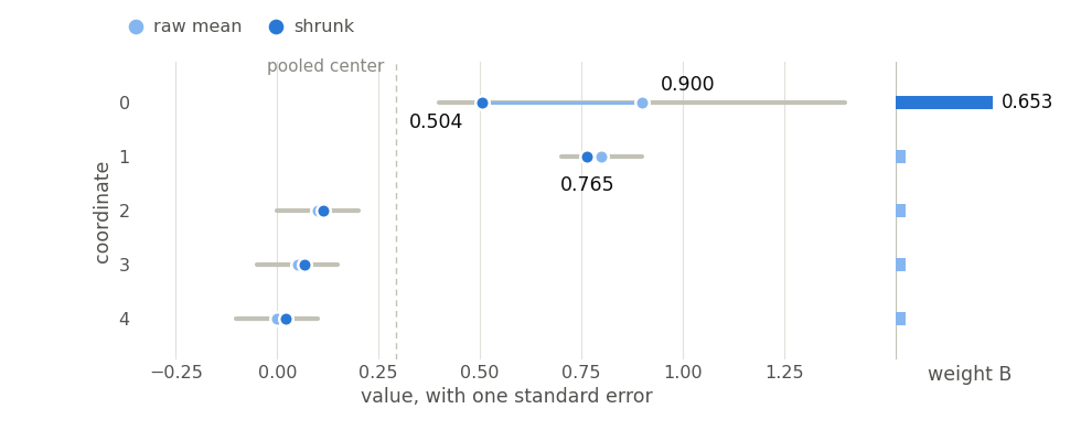
Fig. 2. The noisy leader at coordinate 0 is pulled from 0.90 to 0.504 while the precise 0.80 barely moves, and the order changes
The fitted tau2 is 0.132565 and the pooled center is 0.293961. The leader's weight is 0.6535, so it loses nearly two-thirds of its distance to the center and lands at 0.504. The runner-up's weight is 0.0701 and it holds 0.765. The raw argmax is coordinate 0; the shrunk argmax is coordinate 1. That is the reordering, and it happened because the estimator was told how well each number was measured.
Win rates, and why a proportion needs a transform
A win rate cannot be handed to these estimators directly. It is bounded on both sides, it is not normal, and worst of all its variance p * (1 - p) / n moves with its own value, so the assumption of a variance independent of the mean is violated exactly where it matters. That is a statement about the normal model this header is built on, not a general prohibition: a model made for counts, the beta-binomial hierarchy being the standard choice, shrinks proportions in their own right. Inside the normal framework the classical repair is the arcsine transform, mapping p to 2 * arcsin(sqrt(p)), on which the variance is approximately 1/n.
//+------------------------------------------------------------------+
//| Shrink win rates, or any other proportion                        |
//|                                                                  |
//|  A proportion is not normal and its variance moves with its own  |
//|  value, which breaks the assumption the estimator rests on. The  |
//|  arcsine transform addresses both, mapping to a scale where the  |
//|  variance is about 1/n. The fix is asymptotic, not exact.        |
//+------------------------------------------------------------------+
bool JSShrinkProportions(const double &wins[], const double &n[],
                         double &shrunk[], JSResult &res)
  {
   JSClearResult(res);
   int k = ArraySize(wins);
   res.k = k;

   if(k < 3)
     {
      res.note = "k must be at least 3";
      return(false);
     }
   if(ArraySize(n) != k)
     {
      res.note = "n must have one entry per group";
      return(false);
     }

   double y[], v[];
   ArrayResize(y, k);
   ArrayResize(v, k);

   for(int i = 0; i < k; i++)
     {
//--- every comparison against a NaN is false, so the range test on its
//--- own would pass one through to MathSqrt and MathArcsin
      if(!MathIsValidNumber(wins[i]) || !MathIsValidNumber(n[i]))
        {
         res.note = "every wins and n entry must be finite";
         return(false);
        }
      if(!(n[i] >= 1.0) || wins[i] < 0.0 || wins[i] > n[i])
        {
         res.note = "each group needs n >= 1 and 0 <= wins <= n";
         return(false);
        }
      double p = wins[i] / n[i];
      y[i] = 2.0 * MathArcsin(MathSqrt(p));
      v[i] = 1.0 / n[i];
     }

   double ty[], tf[];
   JSResult inner;
   if(!JSEmpiricalBayes(y, v, ty, tf, inner))
     {
      res.note = inner.note;
      return(false);
     }

   ArrayResize(shrunk, k);
   for(int i = 0; i < k; i++)
     {
      double s = MathSin(ty[i] / 2.0);
      shrunk[i] = s * s;
     }

   res.dof       = inner.dof;
   res.tau2      = inner.tau2;
   res.factor    = inner.factor;
   res.clamped   = inner.clamped;
   res.dominates = inner.dominates;
   res.note      = inner.note;

//--- the target is carried back to the rate scale so the caller
//--- reads a win rate and not an angle
   double st  = MathSin(inner.target / 2.0);
   res.target = st * st;

   res.valid = true;
   return(true);
  }
The function transforms, delegates to the empirical Bayes routine, and maps the result back with sin(y/2) squared. The inverse is exact, so a rate that enters the pipeline comes out as a rate, and the test checks that every output stays inside [0, 1] rather than assuming it. What the transform buys is asymptotic. Normality and the flat 1/n variance are both large-sample approximations, weakest where a trading table reaches for them most: a rate resting against 0 or 1, where the true variance falls below 1/n, and a record of a dozen trades, where nothing has had the chance to become normal. The arcsine scale makes the estimator applicable to proportions; it does not make a thin sample thick.
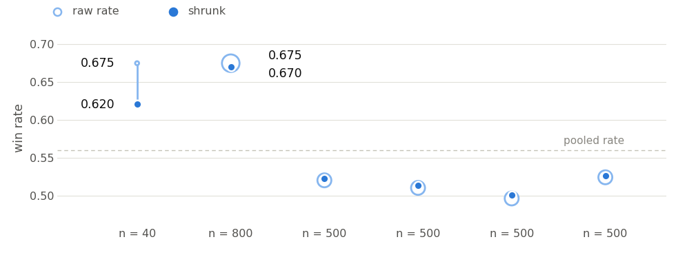
Fig. 3. Two strategies both won 67.5 percent of their trades; the one measured over 40 trades gives back eleven times more than the one measured over 800
The two leftmost pairs are the point of the figure, and the size of the open marker is the reason they behave differently. Both raw rates are 0.675 to three decimals, 27 wins from 40 trades and 540 wins from 800. After shrinkage the thin one reads 0.620 and the thick one reads 0.670, against a pooled rate of 0.5596 and a tau2 of 0.027126. The estimator moved the forty-trade record 0.0545 and the eight-hundred-trade record 0.0049, about eleven to one, because it was told that one of those two numbers is nearly an anecdote.
What shrinkage costs
The theorem promises that the total falls. It promises nothing about any individual coordinate, and the difference deserves a section of its own because it decides whether the estimator is appropriate for a given job.
The test measures it directly. Ten true means are laid out evenly and then scaled until their root mean square distance from their own average is three sigma, 20,000 replications, and three quantities are tracked: the total squared error, the error on the most extreme coordinate, and one near the center.
   for(int r = 0; r < InpReplications; r++)
     {
      for(int i = 0; i < k; i++)
         x[i] = theta[i] + RngNormal();
      JSShrinkToGrandMean(x, sigma2, js, res);

      totRaw += JSTotalSquaredError(x, theta);
      totJS  += JSTotalSquaredError(js, theta);

      double dro = x[outIdx] - theta[outIdx], djo = js[outIdx] - theta[outIdx];
      double drm = x[midIdx] - theta[midIdx], djm = js[midIdx] - theta[midIdx];
      outRaw += dro * dro;
      outJS  += djo * djo;
      midRaw += drm * drm;
      midJS  += djm * djm;
     }

   double n = (double)InpReplications;
   PrintFormat("    total      raw %.5f  js %.5f", totRaw / n, totJS / n);
   PrintFormat("    extreme i  raw %.5f  js %.5f", outRaw / n, outJS / n);
   PrintFormat("    central i  raw %.5f  js %.5f", midRaw / n, midJS / n);

   CheckTrue("total squared error still falls", (totJS < totRaw),
             StringFormat("%.5f vs %.5f", totJS / n, totRaw / n));
   CheckTrue("the extreme coordinate is made worse", (outJS > outRaw),
             StringFormat("%.5f vs %.5f", outJS / n, outRaw / n));
   CheckTrue("a central coordinate is made better", (midJS < midRaw),
             StringFormat("%.5f vs %.5f", midJS / n, midRaw / n));
That block is an excerpt from the middle of the test function; the setup that builds the true means sits above it in the same source file.
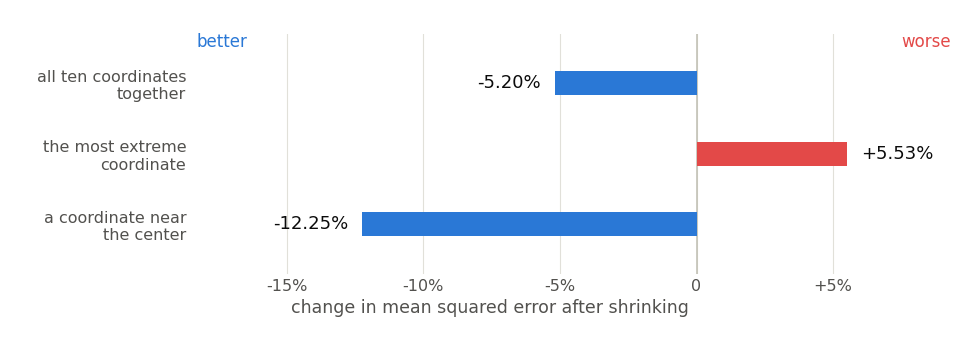
Fig. 4. The total improves from 10.044 to 9.522 while the extreme coordinate degrades from 1.007 to 1.063
The measured numbers are unambiguous. The total falls from 10.044 to 9.522 and the central coordinate improves from 1.008 to 0.885, while the extreme coordinate gets worse, from 1.007 to 1.063. That is not a defect to be tuned away, it is the price the theorem charges. Shrinkage buys accuracy on the ensemble by spending accuracy on the outliers.
Important: if you care about one specific symbol and no other, this estimator is the wrong tool. It is built for the case where the whole table matters, and the coordinate furthest from the center is the one it will hurt.
Verifying the library
Two checks stand behind the numbers in this article. The first recomputes the closed form inside the test itself, so the tolerance can sit at machine epsilon instead of being chosen to make a test pass. The second recomputes everything in a language that shares nothing with MQL5 except the IEEE 754 standard. Both ask whether the code performs the arithmetic it was meant to perform, the second on a second toolchain. Neither derives the statistics independently, so a conceptual error in the estimator would be reproduced by both and reported as agreement.
The closed form, recomputed in the test
//+------------------------------------------------------------------+
//| SECTION 1                                                        |
//|                                                                  |
//|  The formula against arithmetic done here in the open. Nothing   |
//|  external is needed, so the tolerance can sit at machine         |
//|  epsilon instead of being chosen to make a test pass.            |
//+------------------------------------------------------------------+
void Section1_ByHand(void)
  {
   Print("SECTION 1  closed form, recomputed in the test");

   double x[] = {2.0, 4.0, 6.0, 8.0, 10.0};
   double sigma2 = 1.0;
   int    k = ArraySize(x);

//--- grand mean 6, spread 40, dof 2, so the factor is exactly 0.05
   double gm = 6.0;
   double ss = 16.0 + 4.0 + 0.0 + 4.0 + 16.0;
   double bWant = (k - 3) * sigma2 / ss;

   double got[];
   JSResult res;
   bool ok = JSShrinkToGrandMean(x, sigma2, got, res);

   CheckTrue("grand mean call succeeds", ok, "returned " + (string)ok);
   Check("grand mean target", res.target, gm, 1e-15);
   Check("grand mean dof", res.dof, 2.0, 1e-15);
   Check("grand mean factor", res.factor, bWant, 1e-15);

   for(int i = 0; i < k; i++)
     {
      double want = gm + (1.0 - bWant) * (x[i] - gm);
      Check(StringFormat("grand mean shrunk[%d]", i), got[i], want, 1e-15);
     }

//--- the pull is toward the center, so the spread must contract by
//--- exactly the same factor the estimator reported
   double ssAfter = JSSumSquaredDeviation(got, gm);
   Check("spread contracts by (1-B)^2", ssAfter,
         ss * (1.0 - bWant) * (1.0 - bWant), 1e-14);

//--- shrinking is a pull, never a push: the mean cannot move
   Check("grand mean is preserved", JSMean(got), gm, 1e-14);

   double toTarget[];
   JSResult res2;
   JSShrinkToTarget(x, sigma2, 0.0, toTarget, res2);
   double ss0 = 4.0 + 16.0 + 36.0 + 64.0 + 100.0;
   Check("fixed target dof", res2.dof, 3.0, 1e-15);
   Check("fixed target factor", res2.factor, 3.0 * sigma2 / ss0, 1e-15);
  }
The arithmetic here is small enough to do by hand and is written out as such. Five observations at 2, 4, 6, 8 and 10 have a grand mean of exactly 6 and a squared deviation sum of exactly 40, so with k equal to five and unit variance the factor is exactly (5 - 3) / 40, which is 0.05. The invariants that follow would catch a sign error or a wrong denominator: the spread must contract by exactly (1 - B) squared, and the grand mean must not move, because a pull cannot shift the center it pulls toward.
The whole script runs eight such sections. Here is what it reports, and every figure in this article was taken from the same run.
| Section | What it settles | Result |
|---|---|---|
| 1 | Closed form against arithmetic recomputed in the test | factor exactly 0.05, all deviations at or below 2e-16 |
| 2 | The dominance theorem, paired Monte Carlo at k = 10 | raw 10.011, James-Stein 6.811, a 31.96 percent reduction |
| 3 | Risk across eight true spreads from 0 to 16 sigma | 0 of 8 points worse than raw; ratio 0.230 to 0.998 |
| 4 | The k boundary, (k-2) against (k-3) | k = 3 grand mean is bit-exactly equal to the identity on both branches; k = 4 dominates |
| 5 | Empirical Bayes with unequal variances | tau2 recovered as 0.2491 against a true 0.25; ranking reorders |
| 6 | Total improves while an individual degrades | total 10.044 to 9.522, extreme 1.007 to 1.063 |
| 7 | Proportions through the arcsine transform | round trip exact to 1.1e-16; thin sample moves 11 times further |
| 8 | Guards and degenerate inputs | every guard fires; clamped factor collapses to the center |
The closing line of that run reads passed 51, failed 0. Run it yourself with the defaults and you should see the same counts; the Monte Carlo sections are seeded, so the numbers are reproducible rather than merely similar. The seed is the InpSeed input and its default is 20260916. The seeded sections reseed from it in turn, the first from InpSeed itself and the five after it from InpSeed + 1 through InpSeed + 5, so no section inherits the stream the one before it left behind. The generator is xorshift64*, turned into a double with a full 53-bit mantissa because MathRand offers 15 bits and that is not enough to keep an average over 20,000 replications honest. The normals come from the Box-Muller transform, which makes two at a time, and reseeding drops the cached second value so that a reseed cannot hand out a number drawn under the previous seed. Two separate runs of the script agreed on eighty-seven of their eighty-eight lines character for character, and the one line that differed was the elapsed wall clock.
A reference implementation outside MQL5
A test that a library passes against itself shows internal consistency and nothing else. To go further, JS_Export.mq5 writes seven cases to a text file, inputs and outputs together, at seventeen significant digits. That round trips a binary64 exactly, which turns the comparison from an agreement to six decimals into a question of bit equality.
def empirical_bayes(x, v):
    k = len(x)
    tau2 = tau2_dl(x, v)

    sw = 0.0
    swx = 0.0
    for i in range(k):
        w = 1.0 / (tau2 + v[i])
        sw += w
        swx += w * x[i]
    mu = swx / sw

    factor = []
    shrunk = []
    for i in range(k):
        b = v[i] / (tau2 + v[i])
        factor.append(b)
        shrunk.append(mu + (1.0 - b) * (x[i] - mu))
    return tau2, mu, factor, shrunk
The Python is written to match the MQL5 operation for operation. Every sum is an explicit loop, never the builtin sum and never a numpy reduction, because CPython's sum has been compensated since 3.12 and numpy sums pairwise. Either would change the rounding and report a difference that is not a defect. With the order preserved, the two languages are the same IEEE 754 machine and the results should be identical to the last bit. That is a claim about one build on one machine. A fused multiply-add, a different optimization level, or a library computing sqrt, sin or arcsin to a different last bit will each move the comparison off zero, and the response is to read the report in units in the last place rather than relax the threshold.
def ulps(a, b):
    """Distance in representable doubles, which is 0 when bit identical."""
    if a == b:
        return 0
    ia = struct.unpack("<q", struct.pack("<d", a))[0]
    ib = struct.unpack("<q", struct.pack("<d", b))[0]
    if ia < 0:
        ia = -9223372036854775808 - ia
    if ib < 0:
        ib = -9223372036854775808 - ib
    return abs(ia - ib)
The comparison is measured in units in the last place rather than in relative error, and the threshold is zero: anything other than bit equality is a mismatch, so "close enough" never enters the verdict. Run the export, then the cross-check, and the output reads values compared 81, bit identical 81, worst distance 0 ulp. All seven cases agree exactly, including the clamped branch, the branch where tau2 lands on its zero floor, and the arcsine round trip.
On real prices: choosing a Donchian lookback
The library computes what the formulas say it should, on the cases the tests cover. The question that decides whether it is useful is different: does shrinking a table of measured performance help you act on that table? JS_Study.mq5 answers it on eight symbols of H1 data from 2015 to 2025, with no discretion anywhere in the loop.
The data recipe is the script's own defaults, and every part of it is an input rather than a constant. The eight symbols are EURUSD, GBPUSD, USDJPY, AUDUSD, USDCAD, USDCHF, NZDUSD and XAUUSD, read from InpSymbols. The timeframe is PERIOD_H1. The range runs from InpFrom, 2015.01.01, to InpTo, 2025.01.01, and both bounds are fixed dates rather than a count of newest bars, so a rerun covers the same history. The quotes are whatever H1 history the terminal holds for those symbols, which makes the broker part of the recipe: the run quoted here was made on a demo account on the Exness-MT5Trial15 server of Exness Technologies Ltd, MetaTrader 5 build 6182. Those two dates and the bar timestamps are in server time, the clock the bars themselves carry, not GMT and not the local clock. The symbol names have to match the broker's own spelling, which is what the input comment asks for; a server that suffixes its names needs InpSymbols edited before anything will load.
Gaps and session differences are handled by not handling them. CopyRates returns the bars that exist, so weekends, holidays and session breaks are absent rather than filled or interpolated, and a channel breakout can be measured across a gap exactly as it would be in live trading. The walk then counts bars and never calendar time: it steps forward by InpOutSample through one symbol's own array, so window 12 of EURUSD and window 12 of XAUUSD are different stretches of the decade, and a symbol whose sessions are shorter contributes fewer windows to the total. Nothing is aligned across symbols and nothing is resampled. A symbol the broker does not carry is reported and skipped, and so is one holding fewer bars than a single window needs, which at these settings is 2104: the in-sample block, the out-of-sample block, the longest lookback and four spare bars. A reader whose broker carries a different decade of history will get different numbers from the same procedure. What is pinned here is the procedure, the menu and the dates, not the quotes themselves.
The walk-forward design
The menu is eight Donchian stop-and-reverse settings, lookbacks of 10, 14, 20, 28, 40, 55, 75 and 100 bars. Each window ranks all eight on 1500 in-sample bars, picks one, and is scored on the next 500 bars, which the ranking never saw.
Those sizes are inputs too, and the defaults were set from trade supply rather than from results. On H1 the slowest setting on the menu averages 8.1 trades per 1500-bar window, so 1500 bars is close to the floor at which a lookback of 100 still produces a mean and a standard error worth computing; a shorter in-sample block would drop it out of most windows and the eight coordinates would stop being comparable. The 500-bar out-of-sample block doubles as the step, so the windows advance by 500 and overlap by two-thirds, which is the trade between how many windows the decade yields and how dependent those windows are. The five-trade filter is the smallest count worth estimating a variance from, two being the arithmetic floor, and at five it already costs 22 of the 755 windows. No sweep over alternative sizes, timeframes or thresholds was run, so every number in this section is scoped to this configuration. The one result that should be expected to move with it is the collapse of the shrunk pick onto the shortest lookback, because that follows from the spread of the error bars, and the spread of the error bars follows from the trade counts these window sizes produce.
//+------------------------------------------------------------------+
//| A Donchian stop and reverse run over one slice of history        |
//|                                                                  |
//|  The channel is built only from bars that closed before the      |
//|  signal bar, and the fill is taken at the next bar open, so no   |
//|  decision can see a price that had not printed yet.              |
//+------------------------------------------------------------------+
int RunDonchian(const MqlRates &r[], const int a, const int b, const int L,
                double &ret[])
  {
   int n = 0;
   ArrayResize(ret, 0);
   if(b - a <= L + 2)
      return(0);

   int pos = 0, entry = -1, cap = 0;

   for(int t = a + L; t <= b - 2; t++)
     {
      double hh = -DBL_MAX, ll = DBL_MAX;
      for(int j = t - L; j < t; j++)
        {
         if(r[j].high > hh)
            hh = r[j].high;
         if(r[j].low < ll)
            ll = r[j].low;
        }

      int want = pos;
      if(r[t].close > hh)
         want = 1;
      else
         if(r[t].close < ll)
            want = -1;

      if(want != pos)
        {
         if(pos != 0 && entry >= 0)
           {
            double v = pos * (MathLog(r[t + 1].open) - MathLog(r[entry].open));
            if(n + 1 > cap)
              {
               cap = (cap == 0 ? 64 : cap * 2);
               ArrayResize(ret, cap);
              }
            ret[n++] = v;
           }
         pos   = want;
         entry = t + 1;
        }
     }

//--- an open position is closed at the slice edge; one entered on the
//--- final bar never held anything, so it is not counted as a trade
   if(pos != 0 && entry >= 0 && entry <= b - 2)
     {
      double v = pos * (MathLog(r[b - 1].open) - MathLog(r[entry].open));
      if(n + 1 > cap)
        {
         cap = (cap == 0 ? 64 : cap * 2);
         ArrayResize(ret, cap);
        }
      ret[n++] = v;
     }

   ArrayResize(ret, n);
   return(n);
  }
The channel for bar t is built from bars t - L up to t - 1 and never includes bar t itself, and the fill is taken at the open of bar t + 1, so a decision cannot see a price that had not printed when it was made. The end-of-slice flush closes an open position at the slice edge, and the condition that the entry index is at most b - 2 matters more than it looks: without it a reversal signalled on the final bar opens and closes at the same price, a trade returning exactly zero that inflates the trade count and perturbs the standard error the shrinkage depends on.
What that function does not do is charge anything. A trade return is the log of the exit open minus the log of the entry open, signed by the position, with no spread, no commission and no slippage anywhere in the study, so every return quoted in this section is gross. The exposure is worth working out rather than waving at, because the eight settings do not trade equally often.
Charge a constant cost per trade and most of what follows does not move. All eight settings trade the same symbol on the same bar opens under the same reversal fill, so the cost is the same for each of them inside one window. Subtracting a constant from every trade return leaves the sample variance of those returns alone, so each setting keeps the standard error it had, and it shifts all eight in-sample means by that same constant, which leaves tau2 and every per-coordinate weight where they were and moves the pooled center by the constant as well. Both rules therefore pick the settings they pick now, the out-of-sample ranks are read off means per trade and shift together, and the estimation test compares squared differences the constant cancels out of. The rank comparison and the 16.18 percent error reduction are invariant to a flat per-trade cost.
The per-window return is the number that does move, because it is the total of a slice's trades and therefore pays the cost once per trade. A lookback of 10 averages 64.2 in-sample trades per window against 8.1 for a lookback of 100, a factor of 7.9, and the shrunk rule lands on the lookback of 10 in 85.5 percent of windows. A net comparison would charge the shrunk pick several times what it charges a long-lookback pick, which pushes the return difference reported below further against shrinkage rather than in its favor. The study does not model costs, so no net figure is quoted here, and the direction is as far as gross numbers can take it.
   for(int start = 0; start + need <= n; start += InpOutSample)
     {
      int isA = start, isB = start + InpInSample;
      int osA = isB,   osB = isB + InpOutSample;

//--- rank every setting on the in sample slice alone, scanning all of
//--- them so the tally of which ones ran dry counts every failure
      bool usable = true;
      for(int i = 0; i < k; i++)
        {
         double ret[];
         int nt = RunDonchian(r, isA, isB, g_lookback[i], ret);
         g_tradeSum[i] += nt;
         g_tradeCnt[i]++;
         if(nt < InpMinTrades)
           {
            g_skipBy[i]++;
            usable = false;
            continue;
           }
         MeanAndSE2(ret, x[i], v[i]);
         if(!(v[i] > 0.0))
            usable = false;
         else
           {
//--- the error bar and the spread behind it, so the pull each setting
//--- attracts is measured rather than inferred from the trade count
            g_seSum[i] += MathSqrt(v[i]);
            g_sdSum[i] += MathSqrt(v[i] * nt);
            g_seCnt[i]++;
           }
        }
      if(!usable)
        {
         g_skipped++;
         continue;
        }

      JSResult res;
      if(!JSEmpiricalBayes(x, v, shr, bf, res))
        {
         g_skipped++;
         continue;
        }
Each setting supplies a mean return per trade and the squared standard error of that mean, which is what makes the shrinkage per setting rather than uniform: a thinly traded lookback earns a wide error bar and is pulled harder. Those error bars are accumulated as they are produced, which is where the spread from 6.983e-04 to 4.800e-03 quoted earlier comes from.
That standard error is the textbook one, the sample variance of the trade returns over their count, and it treats the trades of one setting in one window as independent draws from one distribution. None of that is quite true on price data. A trending stretch makes consecutive trades of a channel system succeed together, a regime change makes them fail together, and the variance is itself estimated from as few as five numbers. The error bars are therefore optimistic, so the thin settings are pulled less than their uncertainty deserves and the shrinkage below is conservative.
A window where any setting fails to produce five in-sample trades is dropped whole, and the study reports which settings ran dry rather than leaving that to inference. The scan finishes the whole menu even once the window is known to be unusable, so the tally counts every setting that fell short and not only the first one the loop reached. Dropping the whole window keeps the eight coordinates comparable, but the filter is not neutral: a lookback of 100 ran dry in all 22 of the dropped windows, a lookback of 75 in 4 of them, and the six shorter settings in none. The discarded windows are the quiet stretches where a slow channel barely trades, so the study describes periods active enough for all eight settings to trade five times. That is a selection on the data, though at 22 windows out of 755 a small one.
The run attempts 755 windows, drops 22 of them for want of trades, and scores the remaining 733. The two rules agreed on the same setting in 170 of those, so 563 windows carry an actual disagreement to score.
One caveat is required before quoting p-values. The window advances by 500 bars while the in-sample block is 1500, so consecutive windows of one symbol share two-thirds of the bars they are ranked on, and the eight symbols are walked over the same calendar. The 733 rows are not independent. A standard error computed under independence would therefore target the wrong estimate for this design. Every test below is reported twice: once across rows, and once with the residuals summed inside each symbol before they are squared. That correction does not run in one direction. Where a symbol's windows move together the clustered error comes out wider, and where they partly cancel it comes out narrower. Either way it is the one to read, because its assumption matches how the rows were produced. Read it loosely, though: it is asymptotic in the number of clusters, and eight is not a large number. That is why a per-symbol sign test sits beside it wherever a claim rests on the result.
The estimate lands closer
The theorem's own claim, translated to this setting, is that the vector of shrunk means should land closer to what the next slice actually delivered than the vector of raw means does. That is two lines in the loop, and the word translated is carrying weight.
The theorem measures distance to the true means, and nobody observes those. The next slice is a second noisy realization of them, not the truth, so what is measured here is out-of-sample prediction error. Those are two different quantities, and swapping one for the other is a step that has to be paid for rather than waved through. What makes the comparison fair is narrower than the theorem's own claim: the slice's noise is added to both estimators alike, and as long as it is independent of the window the ranking was built on, it cancels in a paired difference. The theorem's setting does not carry over at all. It assumes a known common variance and independent coordinates, and price data offers neither. What follows is a measurement of what shrinkage did on this test bed, under a stationarity the market is under no obligation to honor.
//--- the claim the theorem actually makes, put to real data: which
//--- vector of numbers lands closer to what the next slice delivered
      double eRaw = JSTotalSquaredError(x, oosMean);
      double eShr = JSTotalSquaredError(shr, oosMean);
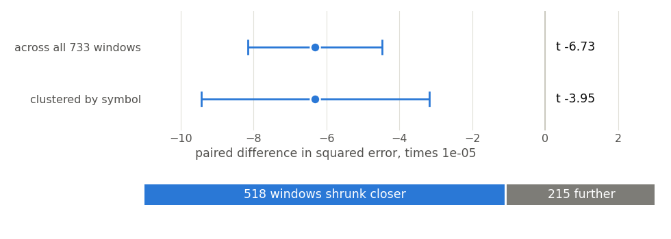
Fig. 5. Shrinking the table of eight means cuts the error against the following slice by 16.18 percent, and wins in 518 of 733 windows
Summed over all eight settings and averaged over the 733 windows, the raw means miss by 3.900e-04 and the shrunk means by 3.269e-04, a reduction of 16.18 percent. The paired difference is -6.312e-05 with a standard error of 9.382e-06, so t is -6.73. Clustering by symbol widens that error to 1.599e-05 and brings t back to -3.95, which is the figure the design supports. Read that one as indicative rather than decisive: a clustered standard error is asymptotic in the number of clusters, and eight is a thin base for one. The shrunk vector was closer in 518 windows and further in 215, and a two-sided sign test returns p below 1e-06.
This is a real effect on real prices, and it is the positive result of the study. On these eight symbols and this decade, the eight numbers an optimizer hands you describe the next period better after they have been shrunk than before.
What selection actually buys
Now the question a trader actually asks. If the shrunk table describes the future better, does picking the top of it beat picking the top of the raw one?
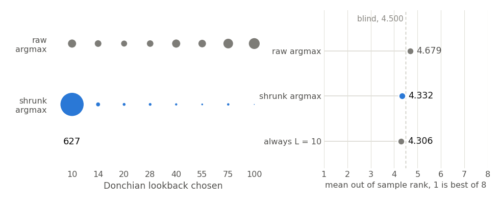
Fig. 6. The shrunk rule lands on the shortest lookback in 627 of 733 windows, and holding that same lookback fixed scores marginally better than the rule itself
On the surface it looks like a win. The shrunk pick finishes at a mean out-of-sample rank of 4.332 against 4.679 for the raw pick, a paired improvement of 0.348 ranks with t equal to 2.92, 3.69 clustered by symbol, and a sign test at p equal to 0.035. Clustering tightened the error bar here rather than widening it, from 0.1191 to 0.0942, because the rank differences inside a symbol partly cancel instead of pointing the same way; the estimation test above went the other way and lost nearly half its t. Asked one symbol at a time, the shrunk rule ranked better in 8 of the 8 symbols, at p equal to 0.008, so the ordering is not an artifact of the overlap.
Blind guessing scores 4.500, and the study tests both rules against it rather than asserting the comparison. The raw rule sits 0.1794 ranks on the wrong side of a coin, at t equal to 2.10 and 2.41 clustered; the shrunk rule sits 0.1685 ranks on the right side, at -2.08 and -2.01 clustered. Both are real but small, roughly two standard errors on a scale running from 1 to 8.
The left panel is what that gain is made of. The raw rule spreads its choices across the whole menu, favoring the long lookbacks that trade rarely and therefore produce the most flattering averages. The shrunk rule picks a lookback of 10 in 627 of 733 windows, which is 85.5 percent. It is barely selecting at all. Shrinkage pulls every mean toward the pooled center in proportion to its own error bar, so the setting with the most trades is left standing while its rivals are dragged in, and the argmax collapses onto the best-measured coordinate. How complete that collapse is depends on the two things that are extreme here: error bars differing by a factor of 6.87, and a between-setting spread the estimator found almost nothing to put in. Give it similar error bars, or a genuine gap between the best and the rest, and the argmax survives. The direction of the pull is what generalizes. A rule weighting each coordinate by its own measured precision moves the winner toward the smallest error bar, and on a menu of one strategy at different speeds that is largely a matter of trade count.
The right panel is where that gain has to be weighed, and the qualification belongs before the number. A rule that ignores the data entirely and always trades a lookback of 10 finishes at a mean rank of 4.306, better than the 4.332 the shrunk rule achieves. But a lookback of 10 is the setting the shrunk rule itself lands on in 85.5 percent of windows, and it was read off the left panel rather than fixed before the study was run. As an out-of-sample competitor it is a post hoc baseline, so the margin of 0.026 ranks is not a result and should never be quoted as though a neutral rule had beaten shrinkage.
Against that pre-specified baseline the shrunk rule is genuinely ahead. What the always-10 line adds is weaker than a defeat and has to be stated at its real strength. It removes the flattering reading of the rank result: every rank the shrunk rule wins over the raw rule is also available from one setting held fixed, which is what you would expect if the rule had found nothing except the lookback with the most trades behind it.
The measured returns are the other half of the picture, and they disagree with the ranks. The shrunk pick averages -0.00280 log return per window against -0.00250 for the raw pick, both gross of execution costs, a paired difference of -0.000304 with t equal to -0.33, -0.40 clustered, and a sign test at p equal to 0.61, better in 275 windows and worse in 288. That is a flat null, and clustering does not move it. Two instruments on one experiment: the rank is the more sensitive and finds a small effect, the log return is what an account receives and finds nothing. Anyone deciding whether to select on a shrunk table is deciding on the second.
Part of the reason sits underneath both rules. The mean Spearman correlation between the in-sample ordering of the eight settings and their out-of-sample ordering is -0.0175. On this test bed the in-sample mean return per trade says essentially nothing about how the settings will be ordered next, so there was little for a rule reading that signal to find. That is a statement about this signal, this menu and this strategy, not a proof that no estimator and no loss function could help selection elsewhere.
What the study does settle is narrower and worth having. Shrinking the table improved the estimate, on every symbol and by a margin that survives clustering the standard error by symbol. Selecting from the shrunk table produced no convincing improvement in profitability, and the selection it did produce reduced the choice to the lookback measured most precisely. The two questions had to be asked separately to get those two answers.
Reading it on a chart: the hour-of-day table
The clearest place to see shrinkage work on live data is an hour-of-day table, and JS_HourEdge.mq5 puts one on a chart. Twenty-four hours, each with its own mean log return and its own standard error over a rolling window, is exactly the unequal-variance case, and picking the best row of such a table is one of the classic ways to fit noise. What runs here is the empirical Bayes form, so its caveat travels with it. Both tau2 and the pooled center are fitted from the same twenty-four hours that are then shrunk, which no dominance theorem covers, and the routine returns dominates as false on every bar it fits. The reason to shrink the table on a live chart is the behavior measured above, not a guarantee.
The table is maintained on sliding accumulators so the cost per plotted bar stays constant.
//+------------------------------------------------------------------+
//| Add or remove one bar's return from its own hour                 |
//|                                                                  |
//|  The window slides one bar at a time, so folding a bar in and    |
//|  out through the same running sums keeps the cost per plotted    |
//|  bar constant instead of rescanning the whole window.            |
//+------------------------------------------------------------------+
void FoldBar(const datetime &time[], const double &close[], const int j,
             const int sign)
  {
   if(j < 1)
      return;
   double prev = close[j - 1];
   if(!(prev > 0.0) || !(close[j] > 0.0))
      return;

   double r = MathLog(close[j] / prev);
   int    h = HourOf(time[j]);
   g_n[h]     += sign;
   g_sum[h]   += sign * r;
   g_sumsq[h] += sign * r * r;
  }
//+------------------------------------------------------------------+ //| Fit the twenty four hours against each other | //| | //| Each hour brings its own mean and its own standard error, and | //| the errors differ because the hours do not carry equal counts | //| or equal volatility. That is the unequal variance case, so the | //| empirical Bayes form is the one that applies. | //+------------------------------------------------------------------+ bool FitHours(double &edgeRaw[], double &edgeShr[], double &weight[], double ¢er, double &tau2, double &meanB, int &kUsed, int &dropped) { double x[], v[]; int hourOf[]; ArrayResize(x, HOURS); ArrayResize(v, HOURS); ArrayResize(hourOf, HOURS); int k = 0; dropped = 0; for(int h = 0; h < HOURS; h++) { edgeRaw[h] = EMPTY_VALUE; edgeShr[h] = EMPTY_VALUE; weight[h] = EMPTY_VALUE; if(g_n[h] < InpMinObs || g_n[h] < 2) { if(g_n[h] > 0) dropped++; continue; } double m = g_sum[h] / g_n[h]; double var = (g_sumsq[h] - g_sum[h] * m) / (g_n[h] - 1); if(!(var > 0.0) || !MathIsValidNumber(var)) { dropped++; continue; } x[k] = m; v[k] = var / g_n[h]; hourOf[k] = h; k++; } kUsed = k; if(k < MIN_GROUPS) return(false); ArrayResize(x, k); ArrayResize(v, k); double shr[], bf[]; JSResult res; if(!JSEmpiricalBayes(x, v, shr, bf, res)) return(false); double bsum = 0.0; for(int j = 0; j < k; j++) { int h = hourOf[j]; edgeRaw[h] = x[j]; edgeShr[h] = shr[j]; weight[h] = bf[j]; bsum += bf[j]; } center = res.target; tau2 = res.tau2; meanB = bsum / k; return(true); }
An hour with fewer than InpMinObs bars in the window, or with a variance that is not finite and positive, is dropped and counted rather than fitted from nothing. The survivors go to the empirical Bayes routine, and the per-hour weight comes back in bf, which is what the panel reports as the pull on the current hour.
//--- the whole pass runs in well under a millisecond, so a tick count
//--- would read zero and look like a stalled fit rather than a fast one
   ulong t0 = GetMicrosecondCount();

//--- prime the accumulators with the window that belongs to the first
//--- plotted bar, which ends on the bar immediately before it
   ResetWindow();
   for(int j = first - InpWindowBars; j <= first - 1; j++)
      FoldBar(time, close, j, +1);

   double edgeRaw[], edgeShr[], weight[];
   ArrayResize(edgeRaw, HOURS);
   ArrayResize(edgeShr, HOURS);
   ArrayResize(weight, HOURS);

   bool any = false;
   for(int i = first; i <= last; i++)
     {
      double center = 0.0, tau2 = 0.0, meanB = 0.0;
      int    kUsed = 0, dropped = 0;

      if(FitHours(edgeRaw, edgeShr, weight, center, tau2, meanB, kUsed,
                  dropped))
        {
         int h = HourOf(time[i]);
         if(edgeShr[h] != EMPTY_VALUE)
           {
            bufShrunk[i] = edgeShr[h] * BP;
            bufColor[i]  = (edgeShr[h] >= 0.0 ? 0.0 : 1.0);
            bufRaw[i]    = edgeRaw[h] * BP;
            bufCenter[i] = center * BP;

            g_edgeRawNow = edgeRaw[h];
            g_edgeShrNow = edgeShr[h];
            g_weightNow  = weight[h];
            g_obsNow     = g_n[h];
            g_hourNow    = h;
            any          = true;
           }
         g_centerNow = center;
         g_tau2Now   = tau2;
         g_meanB     = meanB;
         g_kUsed     = kUsed;
         g_dropped   = dropped;
        }

//--- slide to the next bar: the bar just plotted joins the window and
//--- the oldest one leaves it, so bar i never sees its own return
      if(i < last)
        {
         FoldBar(time, close, i, +1);
         FoldBar(time, close, i - InpWindowBars, -1);
        }
     }
The sliding is the part worth reading closely. The window for the first plotted bar ends on the bar immediately before it. After each bar is plotted it joins the window and the oldest one leaves, so bar i is never in the window used to compute bar i. Every plotted point is a forecast, and the value on the forming bar is what the table says about the hour now opening.
That property is asserted rather than assumed. A separate check recomputes every sampled plotted bar by rescanning its whole window from scratch, the second path a folding error would break, and reports 60 bars compared, 0 differing, worst relative deviation 3.018e-14. The residual is floating point addition not being associative, which is harmless for a display. The same check confirms that every shrunk value lies between its raw value and the pooled center, with zero sign flips and zero overshoot across 600 plotted bars.
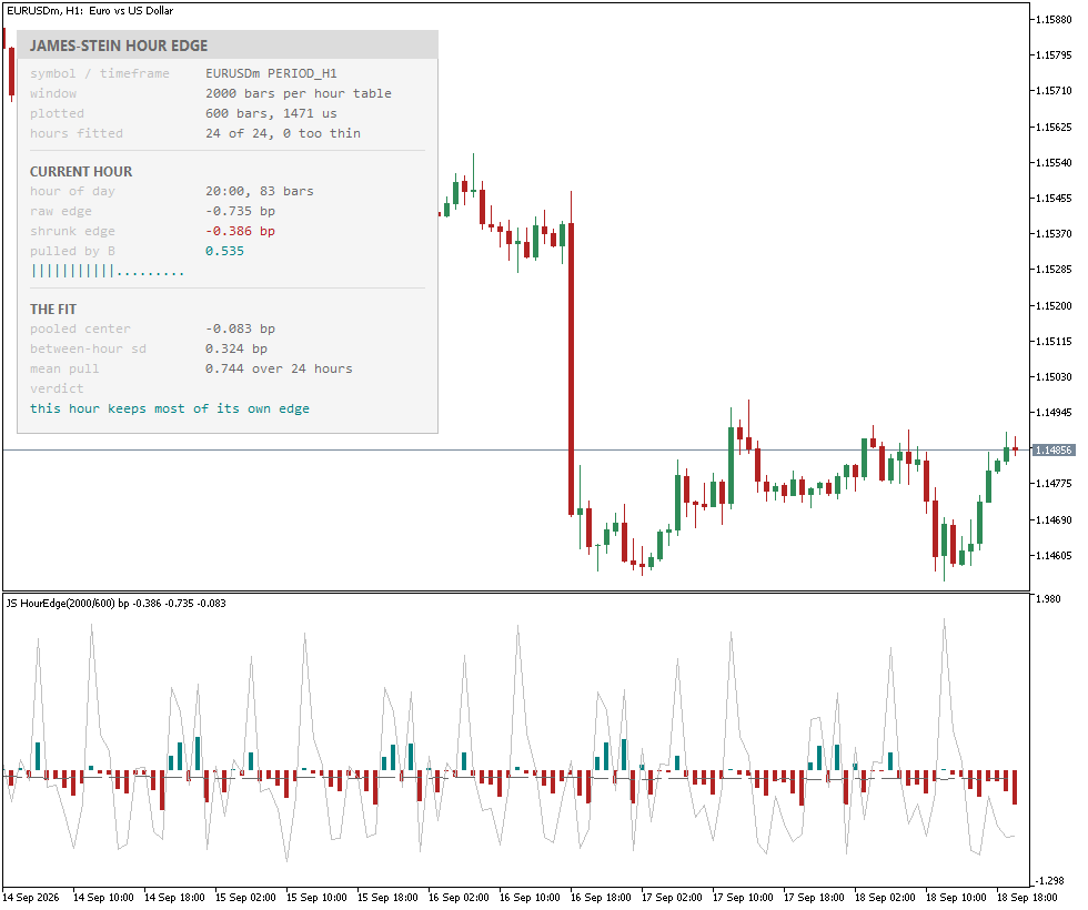
Fig. 7. The raw hourly edge swings across a range the shrunk histogram refuses to follow, with the pooled center drawn as the dashed line both are measured against
Everything on the plot is quoted in basis points, because hourly log returns sit around 1e-05 and are unreadable raw. The silver line is the raw edge of whichever hour each bar opened on, the histogram is the same edge after shrinkage, and the dashed line is the pooled center. The distance between line and bars is the correction, and on a liquid pair it is most of the reading.
The panel reports the fit rather than a trade. It shows how many hours were fitted and how many were too thin, the current hour's raw and shrunk edge, the weight B applied to it, the between-hour standard deviation implied by tau2, and a verdict that speaks only about the estimate: whether this hour keeps its own edge, was mostly pooled away, or whether tau2 landed on its zero floor with no between-hour spread detected.
Conclusion
Shrinkage is one of the few statistical results with a formal proof, and it is also easy to misapply. The proof is narrow. It covers the expected total squared error and not the error on any one draw, assumes a known common variance, says nothing about the coordinate you happen to care about, does not extend to the empirical Bayes form a real table of unequal precisions requires, and has no bearing on selection. Every one of those limits is measured somewhere above. The library implements the estimator four ways, and the study is as clear about where it fails as about where it works.
What the attached files give you:
- A single header with no dependencies: shrinkage toward a fixed target, toward the grand mean, the empirical Bayes form with a variance per coordinate, and a proportions wrapper that handles win rates on the arcsine scale. Each entry point returns a diagnostics struct that reports the weight applied, the fitted tau2, whether the positive part clamped, and whether the configuration is one a dominance theorem actually covers.
- A test script that puts the theorem to work on your own machine: 51 checks over eight sections, the risk curve across eight true separations, the k boundary pinned down to bit-exact agreement on both branches, and every guard made to fire on purpose.
- An export script and a Python reference that agree on all 81 exported values at 0 ulp, which settles that the MQL5 arithmetic is reproduced outside MQL5 and settles nothing about whether the statistics are the right ones.
- A walk-forward study over 733 windows on eight symbols, which measures a 16.18 percent reduction in error against the following slice at t equal to -6.73, or -3.95 once the overlap between windows is priced in, alongside a selection result that carries on the rank scale, vanishes on the return scale, and is matched by one fixed setting identified after the fact.
- An indicator that shrinks a twenty-four-hour table on a live chart, where every plotted point is built only from bars that closed before it.
The practical rule that falls out of the study is short, and it is scoped to the study. Use shrinkage when you want the table itself to be a better description of the next period; over eight symbols and ten years that is what it measurably delivered. Be careful about using it to pick the top row. The argmax of an empirical Bayes vector, fitted with one variance per coordinate and one common center, drifts toward whichever coordinate was measured best, which is arithmetic and not a finding about the market. How far it drifts depends on the spread of the error bars and on how much tau2 finds to work with, both of which the diagnostics report. Ask that of your own table.
| # | Filename | Type | Description |
|---|---|---|---|
| 1 | JamesStein.mqh | Include | The whole library: fixed-target and grand-mean shrinkage, DerSimonian-Laird tau2, empirical Bayes with a variance per coordinate, and proportion shrinkage on the arcsine scale |
| 2 | JS_Test.mq5 | Script | Fifty one checks over eight sections: closed form, the dominance theorem, the risk curve, the k boundary, unequal variances, the individual cost, proportions and the guards |
| 3 | JS_Export.mq5 | Script | Writes seven cases with their inputs and outputs at seventeen significant digits, for comparison outside MQL5 |
| 4 | js_crosscheck.py | Python | Reference implementation outside MQL5; reads the export and compares every value in units in the last place |
| 5 | JS_Study.mq5 | Script | Walk-forward study over eight symbols: does shrinking a table of measured performance improve the estimate, and does it improve the choice |
| 6 | JS_HourEdge.mq5 | Indicator | Hour-of-day edge table shrunk by empirical Bayes, plotted against the raw edge and the pooled center with a panel reporting the fit |
| 7 | MQL5.zip | Archive | Archive with all project files in their subfolders; unpack it into the terminal data directory and every file lands in its required location |
Warning: All rights to these materials are reserved by MetaQuotes Ltd. Copying or reprinting of these materials in whole or in part is prohibited.
This article was written by a user of the site and reflects their personal views. MetaQuotes Ltd is not responsible for the accuracy of the information presented, nor for any consequences resulting from the use of the solutions, strategies or recommendations described.


