Integrating MQL5 with Data Processing Packages (Part 11): Multi-Timeframe Causality Detection using Granger Analysis
 363
 0

Table of Contents
- Introduction
- System Overview
- Getting Started
- Environment and Configuration
- Load the Historical Data
- Feature Engineering
- Label Generation
- Granger F-Test
- Evaluation and Visualization
- Results and Export
- Exploratory Calibration
- Putting it all Together on MQL5
- Where the Live Test Differs from the Notebook
- Backtest
- Conclusion
Introduction
Most multi-timeframe setups rest on an assumption nobody checks: that the higher timeframe tells the lower timeframe something useful. We put an H1 trend filter on an M15 entry, or require M30 and M5 to agree, and move on. Whether the H1 bars actually carry information about the next M15 bar, beyond what the M15 bars already know about themselves, is rarely tested. If that relationship is weak, the extra timeframe is just another condition that cuts trades without improving them. If it is strong only some of the time, a fixed rule will be right in one regime and quietly wrong in the next.
Granger causality is a direct way to test this. The idea is simple: if the past values of series X improve the forecast of series Y beyond what Y's own past already provides, then X "Granger-causes" Y. It says nothing about real-world cause and effect, only about predictive content, and that is exactly the question a trader should ask about a higher timeframe. We run this test in Python, where the statistics tools are mature and easy to cross-check, then carry the result into MQL5 where a simplified version of the same test is recomputed on live data and used as a gate for signals.
The part that makes this interesting is that the result is not guaranteed to be flattering. On EURUSD, under the criterion we set before looking at the output, all four pairs came back INVALID. One pair, M30 -> M15, was promoted to VALID only after we relaxed the stability threshold, which means its status is exploratory rather than a clean pass. Two independent checks in the notebook, a heteroskedasticity-robust test and an out-of-sample comparison, do not support it either. We are keeping the pair in the system so the machinery can be shown end to end, and we say plainly throughout the rest of the article what that costs us in terms of interpretation. For the same reason, the backtest at the end is presented as a demonstration that the pieces work together, not as evidence that the filter improves trading.
System Overview
We split the work into two stages that share one contract: the same alignment rule, and the same lag structure. The first stage runs in Jupyter Lab. We pull OHLC for M5, M15, M30 and H1 from the terminal through the MetaTrader 5 Python package, convert closes to log returns in basis points, and build a design matrix for each pair. For a pair like M30 -> M15, every row is one closed M15 bar. The target is that bar's return. The regressors are the last q M15 returns and the last p completed M30 bar returns. We fit two OLS models, one with only the M15 lags (restricted) and one with the M30 lags added (unrestricted), and compare them with an F-test. Lags are chosen by BIC, significance is corrected across the four pairs with Benjamini–Hochberg, and we check how often the relationship holds on rolling 1,500-bar windows. That rolling share is what we call stability. A pair is VALID when its adjusted p-value is below alpha and its stability clears a threshold. The notebook writes all of this to 'granger_mtf_causality.csv' in the terminal's Common\Files folder.
The second stage is the EA. It reads the CSV on startup, so it knows which pairs to track, which lags to use, and what the offline verdict was. It then repeats the Granger test itself on the most recent 1,500 bars of each pair, every few bars, using a small OLS solver written in MQL5 and the F-distribution from the standard library. The fitted unrestricted model gives a forecast of the current lower-timeframe bar return, and that forecast becomes a vote. The final signal comes from counting votes, but only from pairs whose status is VALID when the filter is on. The EA draws a panel with the status of each pair, can show or hide the signals, publishes the filter state as terminal global variables for other EAs, and can trade the signals with ATR-based stops.
The live test is a simplified version of the offline one, not an exact copy. The MQL5 solver adds a small ridge term, it compares a raw p-value against alpha with no multiple-testing correction, it has no robust-covariance variant, and it looks at one window instead of measuring stability across many. A dedicated section below lists every one of these differences, because "the same test in both places" would be an overstatement.
There is one caveat worth stating up front, because it changes how the whole study should be read. On a single symbol, the higher-timeframe series is not independent. It is constructed from lower-timeframe bars. An M30 log return is the sum of the two M15 log returns inside it, and an H1 return is the sum of four. So the "lead" regressor is a mechanical aggregate of lower-timeframe history, and a significant F-statistic has at least two possible readings. It can mean that longer-horizon structure carries information the short own lags miss. It can also mean the restricted model uses too few own lags. In that case, the higher-timeframe aggregate merely substitutes for omitted M15 lags. Our design cannot separate those two explanations. A fair test of "does an external driver push this market around" needs two different instruments, not two timeframes of one.
Getting Started
Environment and Configuration
The notebook needs MetaTrader 5, pandas, numpy, scipy, statsmodels and matplotlib, all installable with a single pip cell. The terminal must be open and logged in before running. The configuration cell at the top is where the experiment is defined:
SYMBOL          = "EURUSD.m"
DATA_SOURCE     = "mt5"      # "mt5", "csv" or "synthetic"
CSV_DIR         = "./data"   # used when DATA_SOURCE == "csv": files named SYMBOL_TF.csv (time,open,high,low,close)
DAYS_OF_HISTORY = 150
CALIB_END       = None       # last calibration day, e.g. "2025-12-31"; None = up to now

PAIRS = [("H1", "M15"), ("M30", "M15"), ("M15", "M5"), ("H1", "M5")]   # (lead, lag)

ALPHA            = 0.05    # significance level (after BH correction)
MAX_P            = 4       # max lags of the LEAD timeframe (in completed lead bars)
MAX_Q            = 6       # max lags of the LAG timeframe (own returns)
WINDOW           = 1500    # rolling window in lag-TF bars (the EA uses the same window live)
STEP             = 250     # rolling step
STABILITY_MIN    = 0.60    # pre-fixed share of significant rolling windows (0.35 = exploratory only)
TRAIN_FRAC       = 0.70    # chronological train/test split
REQUIRE_OOS_EDGE = False   # if True, VALID also needs a positive out-of-sample directional edge
SCALE            = 1e4     # returns expressed in basis points
'PAIRS' lists the relationships to test, always written as (lead, lag) where the lead is the higher timeframe. WINDOW is shared with the EA: whatever window the notebook uses for its rolling stability scan, the EA uses the same number when re-running the test live. STABILITY_MIN is the threshold that ultimately decided whether M30 -> M15 would be VALID on EURUSD; we will come back to that when the results arrive.
Two values in that cell need a warning label. STABILITY_MIN = 0.60 is the criterion we fixed before running anything, and it produces the main result of this study. A second, exploratory run with STABILITY_MIN = 0.35 supplies the calibration file the EA and the backtest reads; it is described separately under Exploratory Calibration, because that threshold was chosen after seeing the first result. REQUIRE_OOS_EDGE is left at False, which means a pair can be marked VALID even when its out-of-sample behavior is worse than the baseline model. A confirmation run would set it to True; the protocol is given at the end of the backtest section.
CALIB_END pins the last day of calibration data, so the CSV can be built strictly before a backtest starts. Left at None, the window ends at the current date.
'DATA_SOURCE' can be set to "csv" on subsequent runs once the data has been saved, which lets you iterate on the analysis without reconnecting to the terminal every time.
Load the Historical Data
def load_mt5(symbol, tf, days):
    import MetaTrader5 as mt5
    tf_map = {"M1": mt5.TIMEFRAME_M1, "M5": mt5.TIMEFRAME_M5, "M15": mt5.TIMEFRAME_M15,
              "M30": mt5.TIMEFRAME_M30, "H1": mt5.TIMEFRAME_H1, "H4": mt5.TIMEFRAME_H4,
              "D1": mt5.TIMEFRAME_D1}
    end = pd.Timestamp(CALIB_END, tz="UTC") if CALIB_END else pd.Timestamp.now(tz="UTC")
    date_to = (end + pd.Timedelta(days=1)).to_pydatetime()
    date_from = date_to - timedelta(days=days + 1)
    rates = mt5.copy_rates_range(symbol, tf_map[tf], date_from, date_to)
    if rates is None or len(rates) == 0:
        raise RuntimeError(f"No {tf} data for {symbol}: {mt5.last_error()}")
    df = pd.DataFrame(rates)
    df["time"] = pd.to_datetime(df["time"], unit="s")
    # drop the last (still forming) bar so every row is a closed bar
    return df[["time", "open", "high", "low", "close"]].iloc[:-1].reset_index(drop=True)
Our first attempt used copy_rates_from_pos with a bar count sized for a full year. M15, M30 and H1 came back fine, but M5 failed with (-2, 'Terminal: Invalid params') because the requested count exceeded MetaTrаder 5's internal limit. Switching to copy_rates_range with a date window fixed it, and reducing the history to 150 days kept the bar counts manageable. 150 days of M5 is still roughly 25,000 bars, far more than the 1,500-bar rolling window needs.
The iloc[:-1] on the last line matters more than it looks. The most recent bar is still forming, so its close will change. Letting it into the dataset would give the test a small peek at the future on the boundary row. We drop it here so that every row in the returned frame is a confirmed closed bar.
Three sanity checks run on every loaded timeframe before anything else: high must be at or above low on every row, all closes must be positive, and the timestamps must be sorted. They live in the same notebook cell as load_mt5 and run on the data whichever source it came from:
def validate_bars(df, tf):
    # three checks on every timeframe before any test touches the data
    if not (df["high"] >= df["low"]).all():
        raise ValueError(f"{tf}: high below low on some rows")
    if not (df["close"] > 0).all():
        raise ValueError(f"{tf}: non-positive close prices")
    if not df["time"].is_monotonic_increasing:
        raise ValueError(f"{tf}: timestamps are not sorted")
    return df

data = {tf: validate_bars(df, tf) for tf, df in data.items()}
Any violation raises immediately rather than producing a silent bug later in the F-test.
One scheduling detail decides whether this whole study is honest or not. Every table in this article was produced with CALIB_END = None. The last closed bar in the downloaded data was on 21 September 2026, so with DAYS_OF_HISTORY = 150 the calibration window runs from about 24 April to 21 September 2026. The backtest later in the article runs from 1 January 2023 to 31 December 2024, which lies entirely before that window, so the calibration file the EA reads shares no bars with the period it trades. Setting CALIB_END to a date before the first backtest bar achieves the same separation when the test period comes later. The order is unusual, though: the calibration comes from a later period than the test. The backtest therefore asks whether the 2026 verdict carries over to earlier data. It is not a simulation of live use, because nobody trading in 2023 could have known that verdict.

Feature Engineering
Price levels are usually non-stationary, and Granger tests on price levels produce spurious results. The first transformation is to convert each close series to log returns in basis points:
def add_returns(df):
    df = df.copy()
    df["ret"] = SCALE * np.log(df["close"] / df["close"].shift(1))
    return df

data = {tf: add_returns(df) for tf, df in data.items()}

rows = []
for tf in TFS:
    px = data[tf]["close"].tail(5000)
    rt = data[tf]["ret"].dropna().tail(5000)
    rows.append({"tf": tf,
                 "ADF p (price)": adfuller(px, autolag="AIC")[1],
                 "ADF p (returns)": adfuller(rt, autolag="AIC")[1],
                 "ret std (bps)": rt.std()})
adf_table = pd.DataFrame(rows).set_index("tf")
adf_table
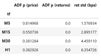
The ADF test is run on both the price and return series for every timeframe. What we expect on this data is a high p-value on prices and a low one on returns, but that is an expectation, not a rule: the ADF outcome depends on the sample period, the test specification and the auto-lag choice, and a trending sample can easily produce a price series that the test rejects. Treat the table as a description of this particular dataset and re-check it whenever you change the symbol or the window, rather than as a box that must tick.
def build_design(tf_lead, tf_lag, p_max=MAX_P, q_max=MAX_Q):
    lo, hi = data[tf_lag], data[tf_lead]
    per_h = pd.Timedelta(minutes=TF_MINUTES[tf_lead])
    y = lo["ret"].to_numpy()
    hret = hi["ret"].to_numpy()
    hpos = np.searchsorted(hi["time"].to_numpy(), (lo["time"] - per_h).to_numpy(), side="right") - 1
    i = np.arange(len(lo))
    ok = (i - q_max >= 1) & (hpos - (p_max - 1) >= 1)
    idx, hp = i[ok], hpos[ok]
    cols = {"y": y[idx]}
    for j in range(1, q_max + 1):
        cols[f"ylag{j}"] = y[idx - j]                 # own lags (lag-TF bars)
    for k in range(1, p_max + 1):
        cols[f"xlag{k}"] = hret[hp - (k - 1)]         # last k completed lead-TF bars
    return pd.DataFrame(cols, index=lo["time"].to_numpy()[idx]).dropna()

designs = {pair: build_design(*pair) for pair in PAIRS}
for pair, D in designs.items():
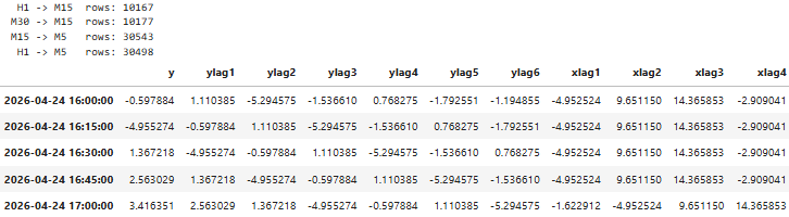
    print(f"{pair[0]:>4} -> {pair[1]:<4} rows: {len(D)}")
designs[PAIRS[0]].head()
The alignment step is the most important part of the whole pipeline, and it is where multi-timeframe work usually goes wrong. For each lower-timeframe bar that opens at time t, we are only allowed to use higher-timeframe bars that had already closed by t. A higher bar closes at its open time plus its period, so the rule is: use higher bars whose open time is at or before t - lead_period.
'searchsorted' with side="right" minus one gives the index of the last higher bar whose open time is at or before the cutoff. From there, xlag1 is the most recent completed higher bar, xlag2 the one before it, and so on.
One design decision here is worth explaining. A more obvious approach would be to forward-fill the higher-timeframe return onto every lower bar and then take ordinary lags of that filled series. The problem is that consecutive lags of a forward-filled series are mostly identical values: four consecutive M15 bars all share the same H1 return, so the lag columns become nearly collinear. Lagging in units of completed higher bars avoids that duplication and is easier to interpret: "do the last p closed M30 bars help predict the next M15 bar?"
It reduces the problem, it does not remove it. Because the higher bar is an aggregate of lower bars on the same symbol, xlag1 and the own lags still overlap mechanically. For M30 -> M15 with q=2, on every row where the M15 bar opens at the top of an M30 bar, xlag1 is exactly ylag1 + ylag2. On the rows where it opens mid-M30, the overlap is partial. So the design matrix contains a column that is, on a repeating subset of rows, a linear combination of columns already in the restricted model. The matrix is not singular, and the regression runs, but the F-test is not cleanly measuring "new information from a higher timeframe" the way it would with two separate instruments.
Label Generation
The target variable y is already defined in build_design: it is the log return of the current lag-timeframe bar in basis points. There is no separate label generation step here the way there would be in a classification pipeline. The Granger test is a regression problem, and the label is the raw return we are trying to forecast. What matters is the sign of the forecast, which becomes the vote direction, and the magnitude relative to the return standard deviation, which is controlled by InpMinEdgeSigma in the EA.
Lags are selected by BIC over a grid of p from 1 to 4 and q from 1 to 6, fitted on the first 70% of each pair's data. On EURUSD, BIC picked p=1 for every pair, with q=2 for M30 -> M15 and q=1 for the others. That is a small model, which is what we would expect when the effect, if any, is modest.
Selecting lags and testing the selected model on the same data inflates significance. The p-value that comes out of granger_test assumes the model was fixed in advance. Ours was not: it won a search over 24 combinations. Nothing in the pipeline corrects for that search, so the reported p-values are optimistic, and the true error rate of the whole procedure is higher than the alpha we compare against. The clean alternatives are to pick p and q on a separate slice of data and never touch them again, or to fix them by argument rather than by search. We mention this here rather than burying it, because it also affects the rolling stability figures that use the same selected lags.
Granger F-Test
The test is the comparison of two nested OLS models:
def granger_test(D, p, q):
    Xr, Xu, y = design_matrices(D, p, q)
    beta_u, rss_u = ols(Xu, y)
    beta_r, rss_r = ols(Xr, y)
    n, k = Xu.shape
    df2 = n - k
    F = max(((rss_r - rss_u) / p) / (rss_u / df2), 0.0)
    return {"F": F, "p_value": float(stats.f.sf(F, p, df2)), "df2": df2,
            "beta_u": beta_u, "beta_r": beta_r, "sigma_y": float(np.std(y))}
The Xr holds a constant plus q own lags. Xu adds the p higher-timeframe lags. If the extra columns reduce the residual sum of squares by more than chance would allow, F is large and the p-value is small.
We wrote this by hand rather than calling grangercausalitytests from statsmodels, because that function assumes both series share the same lag structure and sampling frequency, which is not our case. To verify the implementation, the evaluation cell refits the same models using
sm.OLS(...).compare_f_test(...) and asserts that the p-values match. It also runs an HC3 heteroskedasticity-robust Wald test on the higher-timeframe coefficients, because intraday returns are not homoskedastic and the classical F-test can overstate significance when they are not. That check is not decoration. For M30 -> M15 the classical p-value is 0.0019 and the HC3 p-value is 0.1100, and the second number is the one to believe when residual variance clusters the way intraday returns do. We still report the classical p-value as the headline figure because it is what feeds the VALID rule and what the EA re-computes, but a pair whose significance evaporates under a robust covariance estimator has not really been shown to be significant.
The rolling stability scan repeats the test on every consecutive window of WINDOW bars, stepping forward by STEP each time:
    # rolling stability over the whole sample, same window the EA uses live
    pv, ts = [], []
    for s in range(0, len(D) - WINDOW + 1, STEP):
        w = D.iloc[s:s + WINDOW]
        pv.append(granger_test(w, p, q)["p_value"])
        ts.append(w.index[-1])
    rolling[(lead, lag)] = pd.Series(pv, index=pd.to_datetime(ts))
    stability = float(np.mean(np.array(pv) < ALPHA)) if pv else 0.0
The stability figure is the fraction of windows where the pair was significant. This is the same window the EA re-runs live, so both stages of the system use the same definition.
Treat this number as an activity indicator, not a calibrated statistic. It is affected by three factors: The comparison uses raw p-values with no Benjamini-Hochberg step, so it is more permissive than the headline test. The windows are 1,500 bars long and step 250, so each window shares five sixths of its rows with the next one and the "fraction of significant windows" is an average over heavily dependent tests rather than independent ones. And the lags inside every window are the ones BIC picked on the training slice, which carries the selection problem from the previous section into every point on the curve. A stability of 43% means the relationship shows up in some stretches and not others. It does not mean there is a 43% chance the pair is real.
Finally, p-values across all four pairs are corrected with Benjamini-Hochberg:
res = pd.DataFrame(results)
res["p_adj"] = multipletests(res["p_value"], alpha=ALPHA, method="fdr_bh")[1]
ok = (res["p_adj"] < ALPHA) & (res["stability"] >= STABILITY_MIN)
if REQUIRE_OOS_EDGE:
    ok &= res["oos_edge_bps"] > 0
res["status"] = np.where(ok, "VALID", "INVALID")

assert np.allclose(res["p_value"], res["p_statsmodels"], atol=1e-8), "F-test mismatch with statsmodels"
res.round(5)
The correction is there because we are testing four pairs at once. With four tests at 5%, the probability of at least one false positive is noticeably above 5% without it.
What it covers is exactly those four final tests and nothing else. The lag search, the rolling windows, the threshold we changed after seeing the results, and the separate tester optimizations later in the article are all additional looks at the same data, and none of them enter the correction. Counting only the pieces we can count, the four reported comparisons sit inside a much larger search, so BH here should be read as a minimum adjustment rather than a complete one.
Output:
| lead_tf | lag_tf | p | q | window | alpha | f_stat | p_value | p_statsmodels | p_hc3 | stability | oos_hit | oos_hit_base | oos_edge_bps | oos_r2_gain | n_train | p_adj | status | |
|---|---|---|---|---|---|---|---|---|---|---|---|---|---|---|---|---|---|---|
| 0 | H1 | M15 | 1 | 1 | 1500 | 0.05 | 0.00119 | 0.97252 | 0.97252 | 0.98082 | 0.08571 | 0.52521 | 0.52254 | 0.14268 | -0.00000 | 7116 | 0.97252 | INVALID |
| 1 | M30 | M15 | 1 | 2 | 1500 | 0.05 | 9.64243 | 0.00191 | 0.00191 | 0.11002 | 0.42857 | 0.49967 | 0.51901 | -0.03522 | -0.00575 | 7123 | 0.00764 | VALID |
| 2 | M15 | M5 | 1 | 1 | 1500 | 0.05 | 4.84478 | 0.02774 | 0.02774 | 0.21685 | 0.19658 | 0.50703 | 0.50657 | 0.04416 | 0.00066 | 21380 | 0.05548 | INVALID |
| 3 | H1 | M5 | 1 | 1 | 1500 | 0.05 | 0.09290 | 0.76053 | 0.76053 | 0.83955 | 0.06034 | 0.50492 | 0.50412 | 0.00523 | -0.00000 | 21348 | 0.97252 | INVALID |
This output comes from the exploratory run with STABILITY_MIN = 0.35, described under Exploratory Calibration; under the pre-fixed 0.60, the M30 -> M15 status reads INVALID. Two columns in that table are worth pausing on, because they disagree with the status column for the one pair that the exploratory run passes. For M30 -> M15, p_hc3 is 0.11002 and oos_r2_gain is -0.00575. The second number says the unrestricted model predicted the held-out data worse than the restricted one, which is the opposite of what an informative regressor does.
Evaluation and Visualization
Once all four pairs have been tested, the results table is printed in a format that mirrors the layout of the EA panel. The panel shows the live p-value once the EA has run its own test, so its numbers will differ from the notebook's adjusted values; it is the layout that carries over. This makes it easy to compare the offline notebook verdict against what you later see on the chart.
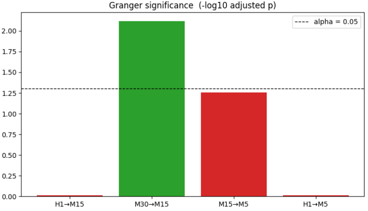
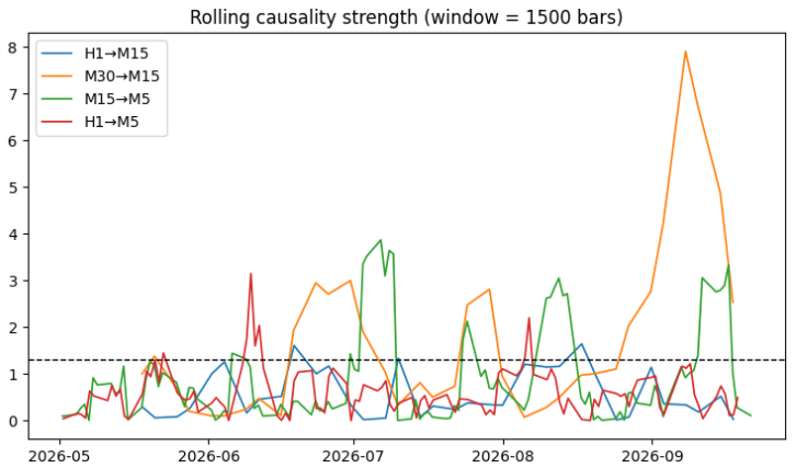
The summary and the two charts in this section were produced in the exploratory run, which is why M30 -> M15 shows as VALID and its bar is green. Under the pre-fixed STABILITY_MIN = 0.60 that status is INVALID and all four bars are red; the bar heights and the rolling curves do not depend on the threshold.
# Step 8 — Monitor-style summary (same layout as the EA panel)
print("MULTI-TIMEFRAME CAUSALITY")
for _, r in res.iterrows():
    print(f"{r.lead_tf:>4} \u2192 {r.lag_tf:<4} {r.status:<8} p_adj={r.p_adj:.4f}  F={r.f_stat:6.2f}  "
          f"stab={r.stability:.0%}  lags(p={r.p}, q={r.q})  OOS hit={r.oos_hit:.1%} vs {r.oos_hit_base:.1%}")
Each line shows the lead and lag timeframe, the VALID or INVALID verdict, the adjusted p-value, the F-statistic, the rolling stability share, the selected lags, and the out-of-sample directional hit rate for both the unrestricted and restricted models. Printing the base hit rate alongside the unrestricted hit rate is deliberate: if the model with higher-timeframe regressors is not beating the own-lags-only model on sign prediction, that is worth knowing before the EA ever trades.

# Step 9 — Visuals for the article
fig, axes = plt.subplots(1, 2, figsize=(15, 4.5))
labels = [f"{a}\u2192{b}" for a, b in zip(res.lead_tf, res.lag_tf)]
colors = ["tab:green" if s == "VALID" else "tab:red" for s in res.status]
axes[0].bar(labels, -np.log10(res["p_adj"].clip(lower=1e-300)), color=colors)
axes[0].axhline(-np.log10(ALPHA), ls="--", c="k", lw=1, label=f"alpha = {ALPHA}")
axes[0].set_title("Granger significance  (-log10 adjusted p)")
axes[0].legend()

for (lead, lag), s in rolling.items():
    axes[1].plot(s.index, -np.log10(s.clip(lower=1e-300)), lw=1.2, label=f"{lead}\u2192{lag}")
axes[1].axhline(-np.log10(ALPHA), ls="--", c="k", lw=1)
axes[1].set_title(f"Rolling causality strength (window = {WINDOW} bars)")
axes[1].legend()
plt.tight_layout()
plt.show()
Step 9 produces the two charts used in the article. The left panel is a bar chart of significance per pair, expressed as negative log10 of the adjusted p-value so that taller bars mean stronger evidence. Bars above the dashed alpha line are significant. The right panel plots the rolling causality strength over time for all four pairs on the same axis, which shows not just whether a relationship exists but when it is active.
The bar color maps directly to status: green for VALID, red for INVALID. On EURUSD, M30 -> M15 is the only green bar. In the rolling chart, the orange M30 -> M15 line is the only one that rises above the dashed threshold with any regularity, and it does so in bursts rather than continuously. Neighbouring points on that curve are computed from windows that share most of their rows, so the line moves smoothly by construction and a burst is fewer independent events than it looks.
Results and Export
Here is what EURUSD produced. This first pass used STABILITY_MIN = 0.60, the value we had set before running anything, and it is the result of the criterion we actually committed to. It is the main, reproducable verdict of this study.
MULTI-TIMEFRAME CAUSALITY
H1 -> M15 INVALID p_adj=0.9725 F= 0.00 stab=9% lags(p=1, q=1) OOS hit=52.5% vs 52.3%
M30 -> M15 INVALID p_adj=0.0076 F= 9.64 stab=43% lags(p=1, q=2) OOS hit=50.0% vs 51.9%
M15 -> M5 INVALID p_adj=0.0546 F= 4.87 stab=20% lags(p=1, q=1) OOS hit=50.7% vs 50.7%
H1 -> M5 INVALID p_adj=0.9725 F= 0.10 stab=6% lags(p=1, q=1) OOS hit=50.5% vs 50.4%
The four INVALID results are not the same kind of INVALID. H1 -> M15 and H1 -> M5 are flat: F near zero, adjusted p near 1, stability under 10%. The hourly timeframe adds nothing to either lower timeframe on this data. M15 -> M5 is borderline at an adjusted p of 0.055 and 20% stability. M30 -> M15 is the interesting case: clearly significant on the training sample (F = 9.64, adjusted p = 0.0076), and it failed only because its rolling stability sat at 43%.
Exploratory Calibration
Everything in this subsection is exploratory. It supplies the calibration file that the EA and backtest read. After the main result came back with no VALID pair, we set STABILITY_MIN to 0.35 and ran the notebook again. Because the data were downloaded again, the newest bars moved the M15 -> M5 and H1 -> M5 figures in the second decimal place; the M30 -> M15 figures did not change, and its status became VALID. It is worth being blunt about what that is. The threshold was moved after seeing which value would change the answer, so the second table below is not an independent test of anything. It is essentially the same data, re-scored with a rule chosen to admit the best-looking pair. Everything downstream of it, including the EA's offline verdict and the backtest, inherits that.
MULTI-TIMEFRAME CAUSALITY
H1 -> M15 INVALID p_adj=0.9725 F= 0.00 stab=9% lags(p=1, q=1) OOS hit=52.5% vs 52.3%
M30 -> M15 VALID p_adj=0.0076 F= 9.64 stab=43% lags(p=1, q=2) OOS hit=50.0% vs 51.9%
M15 -> M5 INVALID p_adj=0.0555 F= 4.84 stab=20% lags(p=1, q=1) OOS hit=50.7% vs 50.7%
H1 -> M5 INVALID p_adj=0.9725 F= 0.09 stab=6% lags(p=1, q=1) OOS hit=50.5% vs 50.4%
Gathering every piece of evidence we have on the one pair that carries the whole system:
| Evidence on M30 -> M15 | Value | Reading |
|---|---|---|
| Classical F-test, BH adjusted | p_adj = 0.0076 | Significant |
| HC3 robust Wald test | p_hc3 = 0.1100 | Not significant |
| Rolling stability | 43% | Below the 60% criterion we set first |
| Out-of-sample hit rate | 50.0% vs 51.9% baseline | Worse than own-lags-only |
| Out-of-sample edge | -0.035 bps | Negative |
| Out-of-sample R2 gain | -0.0058 | Negative |
| Lag selection | BIC over 24 combinations | p-value not corrected for the search |
One test out of several says yes, and it is the one with the weakest assumptions about residual behavior. Setting REQUIRE_OOS_EDGE = True would mark the pair INVALID on the negative out-of-sample edge alone, and so would keeping STABILITY_MIN where it started. The defensible conclusion from the notebook is that no timeframe pair on EURUSD over this window has established Granger causality, and that M30 -> M15 is the only candidate worth watching. We carry it into the EA as an exploratory candidate so the integration can be demonstrated, not because the statistics endorse it.
The last notebook cell writes the table to Common\Files. We write it by hand with \r\n line endings and plain ASCII, because the EA reads it with FILE_TXT | FILE_ANSI and it is easier to control the format directly than to fight pandas defaults:
target = os.path.join(common_files_dir(), OUTPUT_FILE)
write_table(target)
The resulting file has one row per pair: lead_tf, lag_tf, p, q, window, alpha, f_stat, p_value, p_adj, stability, oos_hit, oos_edge_bps, status. Note which p-value the EA actually consumes: it reads column index 8, p_adj, not the raw p_value in column 7. The struct member that stores it is named offlinePAdj in the code below for that reason. The file below, exported from the exploratory run, is the calibration file every EA run in this article reads. It is reproduced in full so the exact inputs are on record. Its M30 -> M15 row carries VALID only under the exploratory threshold; exported under the pre-fixed 0.60, that row reads INVALID and the filter-ON EA would never trade.

Putting it all Together on MQL5
//+------------------------------------------------------------------+
//|                                                   GrangerMTF.mq5 |
//|                                  Copyright 2025, MetaQuotes Ltd. |
//|                     https://www.mql5.com/en/users/johnhlomohang/ |
//+------------------------------------------------------------------+
#property copyright "Copyright 2025, MetaQuotes Ltd."
#property link      "https://www.mql5.com/en/users/johnhlomohang/"
#property version   "1.00"

#include <Trade\Trade.mqh>
#include <Math\Stat\F.mqh>

#define GC_SCALE      10000.0  // returns in basis points (must match SCALE in the notebook)
#define GC_PREFIX     "GCM_"   // chart-object name prefix (panel labels, arrows)
#define GC_GV_PREFIX  "GC_"    // terminal global variables: GC_<symbol>_<lead>_<lag>, GC_<symbol>_SIGNAL

enum ENUM_STATUS_SOURCE
  {
   STATUS_OFFLINE = 0,          // Offline (Jupyter table only)
   STATUS_LIVE    = 1,          // Live (rolling test in MQL5 only)
   STATUS_BOTH    = 2           // Both must agree
  };

//--- inputs
input group "=== Causality Source ==="
input string             InpCausalityFile   = "granger_mtf_causality.csv"; // Calibration file from Jupyter
input bool               InpUseCommonFolder = true;                        // Read from Common\Files
input ENUM_STATUS_SOURCE InpStatusSource    = STATUS_BOTH;                 // How VALID is decided
input int                InpRetestBars      = 12;                          // Re-run live F-test every N lag-TF bars
input string             InpFallbackPairs   = "M30>M15,H1>M15,M15>M5,H1>M5"; // Pairs if file is missing
input int                InpFallbackP       = 1;                           // Fallback lead lags
input int                InpFallbackQ       = 2;                           // Fallback own lags
input int                InpFallbackWindow  = 1500;                        // Fallback window (bars)
input double             InpFallbackAlpha   = 0.05;                        // Fallback alpha
input bool               InpLogParity       = false;                       // Print live F/p on every re-test

input group "=== Signal Generator ==="
input ENUM_TIMEFRAMES    InpSignalTF           = PERIOD_M5; // Signal evaluation timeframe
input bool               InpUseCausalityFilter = true;      // Only VALID pairs may vote
input double             InpMinEdgeSigma       = 0.05;      // Min |forecast| as a fraction of return std
input int                InpMinVotes           = 1;         // Min agreeing votes (with zero opposition)
input bool               InpShowSignals        = true;      // Display signals (panel + chart arrows)
input bool               InpAlertOnSignal      = false;     // Pop-up alert on a new signal

input group "=== Execution ==="
input bool               InpExecuteTrades   = true;   // Trade the internal signals
input double             InpLots            = 0.01;   // Lot size
input int                InpATRPeriod       = 14;     // ATR period (signal TF)
input double             InpSL_ATR          = 1.5;    // Stop loss (x ATR)
input double             InpTP_ATR          = 2.0;    // Take profit (x ATR)
input bool               InpCloseOnOpposite = true;   // Close on an opposite signal
input ulong              InpMagic           = 110011; // Magic number

input group "=== Optimisation ==="
input int                InpMinTradesOpt    = 30;     // OnTester: passes with fewer trades score 0

input group "=== Panel ==="
input bool               InpShowPanel = true;  // Show the causality panel
input int                InpPanelX    = 15;    // Panel X offset
input int                InpPanelY    = 25;    // Panel Y offset
input int                InpFontSize  = 9;     // Panel font size
The EA starts with its inputs, grouped by what they control. The status source decides how VALID is determined: from the Jupyter table alone, from the live test alone, or requiring both to agree. InpShowSignals only affects presentation: the signal line on the panel, the per-pair forecasts and the arrows on the chart. The signal is still computed, published and traded when it is off. Pop-up alerts have their own switch, InpAlertOnSignal, so turning the display off does not silence them. InpUseCausalityFilter is the toggle we will compare in the backtest section.
InpLogParity prints the live F-statistic and p-value every time a pair is re-tested, so the EA can be checked against the notebook on the same window. InpMinTradesOpt feeds a custom criterion in OnTester: recovery factor, with any pass below that trade count scored zero. The optimization reported in this article used the standard Balance max criterion instead; OnTester is there for the confirmation protocol at the end of the backtest section. The two prefixes are kept apart: GC_PREFIX names chart objects only, and GC_GV_PREFIX names the terminal global variables other EAs read.
'InpSignalTF' deserves a note here rather than a surprise later. The statistical work covered M5, M15, M30 and H1, yet the tester optimization behind the backtest settled on PERIOD_M6, a timeframe the analysis never examined and one that does not divide evenly into M15 bars. Setting the signal timeframe below the lag timeframe of a pair does not add information, it only changes how often the same unchanged forecast is looked at. Keeping InpSignalTF equal to the smallest lag timeframe in the pair list is the setting the analysis actually supports.
//--- one lead -> lag relationship
struct SCausalPair
  {
   ENUM_TIMEFRAMES   lead;
   ENUM_TIMEFRAMES   lag;
   string            leadName;
   string            lagName;
   int               p;              // lags of the lead TF (completed lead bars)
   int               q;              // own lags of the lag TF
   int               window;         // rolling window (lag-TF bars)
   double            alpha;
   //--- offline (Jupyter) results
   bool              hasOffline;
   bool              offlineValid;
   double            offlineF;
   double            offlinePAdj;    // BH-adjusted p-value from the notebook (CSV column p_adj)
   double            stability;
   //--- live results
   bool              liveReady;
   double            liveF;
   double            liveP;          // raw p-value of the current window (no BH, no HC3)
   double            beta[];         // unrestricted model: [const, y lags, x lags]
   double            sigmaY;
   datetime          lastLagBar;
   int               barsSinceTest;
   //--- signal state
   double            pred;           // forecast of the current lag-TF bar return (bps)
   int               vote;           // +1 / -1 / 0
   bool              valid;
  };
The two p-value members are named differently on purpose. offlinePAdj holds the BH-adjusted value from the notebook. liveP holds a raw, uncorrected p-value computed from a single window. They are not the same quantity and the next section explains why that matters.
Loading the CSV is plain line-by-line parsing. The file is opened with FILE_COMMON so that both the live terminal and local tester agents can find it. Remote and cloud agents do not have access to the Common folder, so this setup only works with local tester agents.
//+------------------------------------------------------------------+
//| Load the Jupyter calibration table                               |
//+------------------------------------------------------------------+
bool LoadCausalityFile()
  {
   int flags = FILE_READ | FILE_TXT | FILE_ANSI | FILE_SHARE_READ;
   if(InpUseCommonFolder)
      flags |= FILE_COMMON;

   int h = FileOpen(InpCausalityFile, flags);
   if(h == INVALID_HANDLE)
     {
      PrintFormat("Causality file '%s' not found (error %d). Using fallback pairs.",
                  InpCausalityFile, GetLastError());
      return false;
     }

   int line = 0;
   while(!FileIsEnding(h))
     {
      string row = FileReadString(h);
      line++;
      if(line == 1)
         continue;                               // header
      StringTrimLeft(row);
      StringTrimRight(row);
      if(StringLen(row) == 0)
         continue;

      string f[];
      if(StringSplit(row, ',', f) < 13)
         continue;

      ENUM_TIMEFRAMES lead = TfFromString(f[0]);
      ENUM_TIMEFRAMES lag  = TfFromString(f[1]);
      if(!AddPair(lead, lag, (int)StringToInteger(f[2]), (int)StringToInteger(f[3]),
                  (int)StringToInteger(f[4]), StringToDouble(f[5])))
         continue;

      int i = g_pairCount - 1;
      string status = f[12];
      StringTrimLeft(status);
      StringTrimRight(status);
      g_pairs[i].hasOffline   = true;
      g_pairs[i].offlineF     = StringToDouble(f[6]);
      g_pairs[i].offlinePAdj  = StringToDouble(f[8]);   // f[8] is p_adj, not p_value
      g_pairs[i].stability    = StringToDouble(f[9]);
      g_pairs[i].offlineValid = (status == "VALID");
     }
   FileClose(h);
   return (g_pairCount > 0);
  }
If the file is missing, the EA falls back to the pairs, lags and window from the inputs and uses the live test alone for validity. AddPair also rejects pairs where the lead is not the higher timeframe, or where the window is too short for the number of coefficients.
The live test is where most of the work happens. RunGranger copies enough bars of both timeframes, rebuilds the same design matrix the notebook built, and computes the same F-statistic on it:
//+------------------------------------------------------------------+
//| Live Granger F-test                                              |
//+------------------------------------------------------------------+
bool RunGranger(SCausalPair &cp)
  {
   const int p = cp.p;
   const int q = cp.q;
   const int W = cp.window;
   const int k = 1 + q + p;

   int needLow = W + q + 3;
   MqlRates lo[];
   ArraySetAsSeries(lo, true);
   if(CopyRates(_Symbol, cp.lag, 0, needLow, lo) < needLow)
      return false;

   int ratio    = MathMax(1, PeriodSeconds(cp.lead) / PeriodSeconds(cp.lag));
   int needHigh = needLow / ratio + p + 20;
   MqlRates hi[];
   ArraySetAsSeries(hi, true);
   int gotHigh = CopyRates(_Symbol, cp.lead, 0, needHigh, hi);
   if(gotHigh < p + 3)
      return false;

   int    perH = PeriodSeconds(cp.lead);
   double X[], Y[];
   ArrayResize(X, W * k);
   ArrayResize(Y, W);

   int    n = 0, h = 0;
   double sumY = 0.0, sumY2 = 0.0;
   for(int s = 1; s <= W; s++)
     {
      if(s + q + 1 >= needLow)
         break;
      datetime cutoff = lo[s].time - perH;       // lead bar must have closed by lo[s].time
      while(h < gotHigh && hi[h].time > cutoff)
         h++;
      if(h + p >= gotHigh)
         break;

      int o = n * k;
      X[o] = 1.0;
      for(int j = 1; j <= q; j++)
         X[o + j] = LogRet(lo, s + j);
      for(int m = 1; m <= p; m++)
         X[o + q + m] = LogRet(hi, h + m - 1);
      Y[n]   = LogRet(lo, s);
      sumY  += Y[n];
      sumY2 += Y[n] * Y[n];
      n++;
     }
Both arrays are in series order, with index 0 being the forming bar and index 1 the most recent closed bar. The loop walks back through the last W closed lower bars. The cutoff rule is the same as in Python: a higher bar only counts if it closed before the lower bar opened. Since the lower bars move back in time as s increases, the matching higher-bar pointer h can only move forward, so a single pointer through the high array is enough with no search per row.
LogRet returns 10000 * ln(close[i] / close[i+1]), the MQL5 twin of the notebook's SCALE * np.log(...). If this function and the notebook ever disagree on the scale or on which bar is used, the coefficients learned in Python mean nothing in MQL5. We kept them deliberately identical.
The design matrix is stored flat, n rows by k columns. FitOLS builds X'X and X'y, adds a small ridge term to the diagonal to keep the system well-conditioned, and solves it with Gaussian elimination with partial pivoting. MQL5 has matrix types now, but a hand-written solver keeps the logic visible, and with at most a dozen coefficients the cost is negligible. The restricted model is fitted from the same flat matrix using only its first 1 + q columns, so both models see exactly the same rows.
   if(n < 5 * k)
      return false;

   double betaU[], betaR[];
   double rssU = 0.0, rssR = 0.0;
   if(!FitOLS(X, Y, n, k, k, betaU, rssU))
      return false;
   if(!FitOLS(X, Y, n, k, 1 + q, betaR, rssR))
      return false;

   int    df2   = n - k;
   double fStat = (rssU > 0.0) ? ((rssR - rssU) / p) / (rssU / df2) : 0.0;
   if(fStat < 0.0)
      fStat = 0.0;

   int    err = 0;
//--- upper tail P(F >= fStat), the same quantity as scipy.stats.f.sf
   double pv = MathCumulativeDistributionF(fStat, (double)p, (double)df2, false, false, err);
   if(err != 0 || !MathIsValidNumber(pv))
      pv = 1.0;                                  // fail towards "no causality"

   cp.liveF = fStat;
   cp.liveP = MathMin(MathMax(pv, 0.0), 1.0);
   if(InpLogParity)
      PrintFormat("PARITY %s->%s last_closed=%s n=%d F=%.6f p=%.8f",
                  cp.leadName, cp.lagName, TimeToString(lo[1].time), n, fStat, cp.liveP);
   ArrayCopy(cp.beta, betaU);
   double mean = sumY / n;
   cp.sigmaY    = MathSqrt(MathMax(sumY2 / n - mean * mean, 0.0));
   cp.liveReady = true;
   return true;
  }
The p-value line is the one place where the two stages could silently disagree, so it is worth being precise about. scipy's stats.f.sf returns the upper tail, P(F ≥ fStat), which is what a Granger test needs. MathCumulativeDistributionF in <Math\Stat\F.mqh> takes a tail flag whose meaning is easy to misread, and in the library source that flag is documented as the switch for the lower tail. So tail = true returns P(F ≤ fStat), and passing true and then taking 1.0 - cdf would also give the right number. We pass tail = false instead, which asks the library for the upper tail directly, removes a subtraction the reader has to reason about and avoids losing digits when the p-value is very small. If anything goes wrong in the calculation, the p-value defaults to 1.0, which makes the pair INVALID. Failing towards "no causality" is the safer direction for a filter.
A flipped tail would invert every VALID decision without a single error message. The EA checks the function against known values before it does anything else:
//+------------------------------------------------------------------+
//| Startup self-test of the F-distribution tail                     |
//+------------------------------------------------------------------+
bool CheckFDistribution()
  {
   int    e1 = 0, e2 = 0;
   double pSmall = MathCumulativeDistributionF(1.0,  1.0, 1000.0, false, false, e1);
   double pLarge = MathCumulativeDistributionF(10.0, 1.0, 1000.0, false, false, e2);
   PrintFormat("F-tail check: P(F>=1)=%.7f (scipy 0.3175524)  P(F>=10)=%.7f (scipy 0.0016126)",
               pSmall, pLarge);
   if(e1 != 0 || e2 != 0)
      return false;
   if(MathAbs(pSmall - 0.3175524) > 1e-5 || MathAbs(pLarge - 0.0016126) > 1e-6)
      return false;
   return (pLarge < pSmall);                     // an upper tail must fall as F grows
  }
The two reference values are scipy.stats.f.sf(1.0, 1, 1000) and scipy.stats.f.sf(10.0, 1, 1000). A correct upper tail gives about 0.3176 and 0.0016 and falls as F grows; a lower tail would give 0.6824 and 0.9984 and rise. OnInit calls this first and returns INIT_FAILED on a mismatch, and it prints both values to the Experts log, so anyone reproducing the EA can see the check pass rather than take our word for it.
The ridge term in FitOLS is a deliberate compromise. It keeps X'X invertible under near-collinearity. However, it also means the residuals and the resulting F-statistic are only approximate. The F-ratio built from those residuals is therefore an approximation of the classical statistic rather than the statistic itself. At 1e-9 relative to return variances measured in basis points the distortion is small, and you can set it to zero and rely on the pivoting if you prefer the textbook quantity with a small risk of a failed solve.
We do not re-run this test on every bar. On a year of M5 data, four pairs and 1,500-row regressions on every tick would make the tester crawl for no real benefit, since the window barely changes from one bar to the next. InpRetestBars controls how often each pair is retested, counted in its own lower-timeframe bars. With the default of 12, an M15 pair retests every three hours.
The forecast runs on every new signal bar and is simple, since it only applies the already-fitted coefficients to the current state of both timeframes:
//+------------------------------------------------------------------+
//| Forecast the current lag-TF bar from closed bars only            |
//+------------------------------------------------------------------+
bool ComputePrediction(SCausalPair &cp)
  {
   cp.pred = 0.0;
   cp.vote = 0;
   if(!cp.liveReady)
      return false;

   const int p = cp.p;
   const int q = cp.q;

   MqlRates lo[];
   ArraySetAsSeries(lo, true);
   if(CopyRates(_Symbol, cp.lag, 0, q + 2, lo) < q + 2)
      return false;

//--- most recent lead bar that closed at or before the current lag bar opened
   datetime cutoff = lo[0].time - PeriodSeconds(cp.lead);
   int h0 = iBarShift(_Symbol, cp.lead, cutoff, false);
   if(h0 < 0)
      return false;
   while(iTime(_Symbol, cp.lead, h0) > cutoff)
      h0++;
   while(h0 > 0 && iTime(_Symbol, cp.lead, h0 - 1) <= cutoff)
      h0--;

   MqlRates hi[];
   ArraySetAsSeries(hi, true);
   if(CopyRates(_Symbol, cp.lead, h0, p + 1, hi) < p + 1)
      return false;

   double f = cp.beta[0];
   for(int j = 1; j <= q; j++)
      f += cp.beta[j] * LogRet(lo, j);
   for(int m = 1; m <= p; m++)
      f += cp.beta[q + m] * LogRet(hi, m - 1);

   cp.pred = f;
   double thr = InpMinEdgeSigma * cp.sigmaY;
   if(f > thr)
      cp.vote = 1;
   else
      if(f < -thr)
         cp.vote = -1;
   return true;
  }
The two while loops after iBarShift are a guard against timing boundary cases. We want the last higher bar whose open time is at or before the cutoff, and rather than rely on exactly how iBarShift resolves a time that falls between bars, we correct the index in both directions. The vote threshold is a fraction of the return standard deviation from the live window, so the same InpMinEdgeSigma input works across pairs whose returns have different scales.
The forecast is for a whole lag-timeframe bar, and it does not change until that bar closes, because none of its inputs change inside the bar. When the signal timeframe is smaller than the lag timeframe, the same unchanged number is therefore re-read on every signal bar: an M15 pair evaluated on M5 votes three times on one forecast, and on M2 it votes seven or eight times. A position opened on the last of those votes is acting on a prediction for a bar that has nearly finished. Pairs with different lag timeframes are also voting on different clocks while being counted into one signal, so the votes are not equally fresh. Running the signal timeframe equal to the smallest lag timeframe keeps this to one vote per forecast per pair.
The status logic combines the offline and live verdicts:
//+------------------------------------------------------------------+
//| VALID / INVALID decision                                         |
//+------------------------------------------------------------------+
void UpdateValidity(SCausalPair &cp)
  {
   bool live    = cp.liveReady && cp.liveP < cp.alpha;
   bool offline = cp.hasOffline && cp.offlineValid;

   switch(InpStatusSource)
     {
      case STATUS_OFFLINE:
         cp.valid = cp.hasOffline ? offline : live;
         break;
      case STATUS_LIVE:
         cp.valid = live;
         break;
      default:
         cp.valid = cp.hasOffline ? (offline && live) : live;
         break;
     }
  }
With STATUS_BOTH, a pair needs the notebook's approval and a significant result on the current live window. "Significant" means something weaker here than it does in the notebook, which is the subject of the next section. STATUS_BOTH is the setting to use precisely because the offline half of the condition carries the stricter criterion; STATUS_LIVE on its own applies the loosest rule in the whole system. Every backtest in this article was run with STATUS_BOTH. STATUS_LIVE is kept as a diagnostic, for watching how often the live test alone would fire, and its results should not be used to judge performance.
The signal generator is intentionally plain. Each pair casts a vote of +1, -1 or 0, and the filter decides who is allowed to vote:
//+------------------------------------------------------------------+
//| Combine the pair votes into one BUY / SELL / NONE signal         |
//+------------------------------------------------------------------+
int AggregateSignal()
  {
   g_bulls = 0;
   g_bears = 0;
   for(int i = 0; i < g_pairCount; i++)
     {
      if(!g_pairs[i].liveReady)
         continue;
      if(InpUseCausalityFilter && !g_pairs[i].valid)
         continue;
      if(g_pairs[i].vote > 0)
         g_bulls++;
      if(g_pairs[i].vote < 0)
         g_bears++;
     }
   if(g_bulls >= InpMinVotes && g_bears == 0)
      return 1;
   if(g_bears >= InpMinVotes && g_bulls == 0)
      return -1;
   return 0;
  }
With the filter off, all four pairs vote including the ones the statistics say carry no information. With the filter on, only VALID pairs vote. A signal needs at least InpMinVotes agreeing votes with zero opposition. Keeping this logic simple was deliberate: if the voting scheme were clever, it would be hard to tell whether a difference between the two runs came from the causality filter or from the voting itself.
//+------------------------------------------------------------------+
//| Expert tick function                                             |
//+------------------------------------------------------------------+
void OnTick()
  {
   datetime t = iTime(_Symbol, InpSignalTF, 0);
   if(t == 0 || t == g_lastSigBar)
      return;
   g_lastSigBar = t;

   for(int i = 0; i < g_pairCount; i++)
     {
      datetime lb = iTime(_Symbol, g_pairs[i].lag, 0);
      if(lb != g_pairs[i].lastLagBar)
        {
         g_pairs[i].lastLagBar = lb;
         g_pairs[i].barsSinceTest++;
        }
      if(!g_pairs[i].liveReady || g_pairs[i].barsSinceTest >= InpRetestBars)
        {
         if(RunGranger(g_pairs[i]))
            g_pairs[i].barsSinceTest = 0;
        }
      ComputePrediction(g_pairs[i]);
      UpdateValidity(g_pairs[i]);
     }

   int  signal      = AggregateSignal();
   bool isNewSignal = (signal != 0 && signal != g_lastSignal);

   ExportGlobals(signal);

   if(isNewSignal)
     {
      if(InpShowSignals)
         DrawSignalArrow(signal, t);
      if(InpAlertOnSignal)
         Alert(StringFormat("%s Granger MTF signal: %s", _Symbol, signal > 0 ? "BUY" : "SELL"));
     }

   if(InpExecuteTrades)
      ManageTrades(signal, isNewSignal);

   g_lastSignal = signal;
   UpdatePanel(signal);
  }
//+------------------------------------------------------------------+
OnTick ties everything together on each new signal bar. Pairs are re-tested when due, forecasts are refreshed, statuses updated, and the signal is aggregated. A trade opens only when the signal changes, so a BUY that stays BUY for twenty bars produces one entry, not twenty. Arrows depend on InpShowSignals and pop-up alerts on InpAlertOnSignal; neither affects whether a signal is traded.
//+------------------------------------------------------------------+
//| Publish filter state for other EAs (terminal global variables)   |
//+------------------------------------------------------------------+
void ExportGlobals(const int signal)
  {
   for(int i = 0; i < g_pairCount; i++)
      GlobalVariableSet(GC_GV_PREFIX + _Symbol + "_" + g_pairs[i].leadName + "_" + g_pairs[i].lagName,
                        g_pairs[i].valid ? 1.0 : 0.0);
   GlobalVariableSet(GC_GV_PREFIX + _Symbol + "_SIGNAL", (double)signal);
  }
ExportGlobals publishes the filter state as terminal global variables. The names follow GC_<symbol>_<lead>_<lag> for each pair and GC_<symbol>_SIGNAL for the combined signal, where <symbol> is _Symbol exactly as the terminal reports it, broker suffix included. On the server used here that gives GC_EURUSD.m_M30_M15 and GC_EURUSD.m_SIGNAL. Pair values are 1.0 for VALID and 0.0 for INVALID; the signal is 1.0, -1.0 or 0.0. GCM_ is a separate prefix that only names the panel labels and chart arrows. Another EA on the same symbol reads the filter with GlobalVariableGet("GC_" + _Symbol + "_M30_M15") and needs no shared code. ManageTrades opens positions with stop loss and take profit as ATR multiples on the signal timeframe, respects the broker's stop level, and optionally closes an open position when the opposite signal appears.
Where the Live Test Differs from the Notebook
It would be convenient to say the EA runs the same test as the notebook. It does not, and the differences all point the same way: the live criterion is easier to pass. They are collected here so nobody has to reverse-engineer them from the code.
| Step | Notebook | EA | Effect on the live verdict |
|---|---|---|---|
| Solver | Plain OLS (numpy lstsq) | Normal equations with a 1e-9 ridge | Coefficients very slightly shrunk; the F-ratio is an approximation of the classical statistic |
| Multiple testing | Benjamini-Hochberg across the four pairs | None; raw p compared to alpha | More false positives, growing with the number of pairs tracked |
| Robust covariance | HC3 Wald test reported alongside | Not implemented | Heteroskedasticity is not accounted for live, and it is what killed M30 -> M15 offline |
| Stability | Fraction of significant rolling windows | Current window only | A single lucky window can flip a pair to VALID |
| Out-of-sample check | Held-out 30% hit rate and R2 gain | Not implemented | No live guard against a model that fits in-window and fails out of it |
| Retest frequency | Every STEP bars over history | Every InpRetestBars lag-TF bars | Different sampling of the same curve; not a mismatch in itself |
| Tail probability | stats.f.sf (upper tail) | MathCumulativeDistributionF with tail = false, verified at startup | Same quantity; checked against scipy reference values, not assumed |
Two of these are easy to fix if you want the live rule to resemble the offline one. Comparing liveP against alpha divided by the number of tracked pairs applies a Bonferroni correction, which is stricter than BH and takes one line in AddPair. Keeping a short ring buffer of the last N live test outcomes per pair and requiring a minimum share of them to be significant reproduces the stability criterion live. Neither is in the build used for the backtest below, so treat them as the obvious next step rather than as results.
Until they are in, STATUS_BOTH is doing most of the work: the offline flag carries the stricter criterion, and the live flag only adds the requirement that the current window still looks significant. One more guard comes through the same route. With REQUIRE_OOS_EDGE = True in the notebook, a pair whose out-of-sample edge is negative is exported as INVALID, and under STATUS_BOTH the EA refuses it whatever the live window says. That is the setting a confirmation run should use.
Backtest
The backtest is an exploratory engineering demonstration, not an independent validation of trading performance. One parameter set is run twice over the same period, and the only input that changes between the two runs is InpUseCausalityFilter. Run A has the filter on, so only VALID pairs may vote. Run B has it off, so all four pairs vote. Both runs read the same calibration file, the exploratory one described under Exploratory Calibration, and the test period, 1 January 2023 to 31 December 2024, lies entirely before that file's calibration window. Two things limit what the runs can show. The parameter set was optimized on the same 2023 to 2024 period it is tested on, so the results are in-sample. The calibration comes from 2026, after the test period, so the runs are not a historically realistic simulation either: nobody trading in 2023 could have known that calibration.
Settings
The results below were achieved with the settings below, with only InpUseCausalityFilter toggled:
| Input | Value |
|---|---|
| InpStatusSource | STATUS_BOTH (both must agree) |
| InpRetestBars | 12 |
| InpSignalTF | M6 |
| InpMinEdgeSigma | 0.125 |
| InpMinVotes | 1 |
| InpLots | 0.10 |
| InpATRPeriod | 104 |
| InpSL_ATR | 9.3 |
| InpTP_ATR | 5.6 |
| InpCloseOnOpposite | false |
| InpUseCausalityFilter | Run A: true | Run B: false |
Results
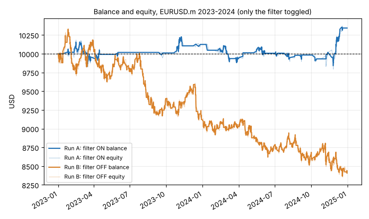
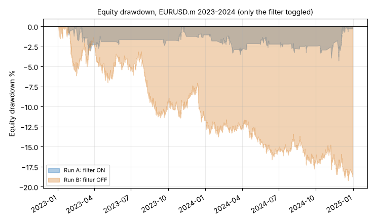
Below are the equity curve and drawdown for both Run A and Run B:
Now the summarized backtest for both Run A and Run B:
| Metric | Run A (filter ON) | Run B (filter OFF) |
|---|---|---|
| Net profit | +342.95 | -1,568.54 |
| Gross profit | 3,422.76 | 12,360.31 |
| Gross loss | -3,079.81 | -13,928.85 |
| Profit factor | 1.11 | 0.89 |
| Recovery factor | 0.78 | -0.79 |
| Max equity drawdown | $437.91 (4.28%) | $1,987.56 (19.22%) |
| Total trades | 238 | 952 |
| Win rate | 63.9% | 61.0% |
| Avg win / Avg loss | 22.52 / -35.81 | 21.27 / -37.54 |
| Max consecutive losses | 3 | 10 |
| LR correlation (balance) | 0.164 | -0.959 |
With nothing else changed, the filter cut the number of trades from 952 to 238. Run A finished with a profit of 342.95 and Run B with a loss of 1,568.54, and the maximum drawdown was 4.28% against 19.22%. Run A ended both 2023 and 2024 above its starting balance for the year, and Run B ended both below. The mechanism is visible in the trade averages. Because the exit settings are identical, the average win and average loss barely move between the runs, so the difference has to come from which trades are taken. With a stop of 9.3 ATR against a target of 5.6 ATR, the average loss is larger than the average win, and the win rate needed to break even is about 61.4% for Run A and 63.8% for Run B. Run A clears its break-even rate by about two and a half points, and Run B misses its own by about the same margin. The whole difference lives in a few points of win rate, gained by letting only the M30 -> M15 pair vote. These are in-sample figures from an exploratory run and should not be read as evidence of validated trading performance.
What this test does not show:
- That M30 -> M15 carries real information. Its VALID flag comes from the exploratory calibration, under a threshold relaxed after seeing the main result.
- That the improvement is about causality rather than trading less. The filter removes three quarters of the trades from a configuration that loses money without it, and a placebo run with the VALID flag forced onto a rejected pair has not been done. Neither has a comparison against an unfiltered run thinned to the same trade frequency.
- Out-of-sample performance. The parameters were optimized on the same period the runs cover, so a chronologically correct out-of-sample or walk-forward test would be needed before any claim about trading effectiveness.
- A historically realistic result. The calibration file was built from 2026 data, after the 2023 to 2024 test period.
- Robustness of the chosen parameters. The optimized signal timeframe, M6, is not one of the timeframes the notebook analysed, and no neighbouring-parameter check was run.
Optimization Protocol
The optimization ran on 1 January 2023 to 31 December 2024 with the Fast genetic based algorithm, over the grid below, with Balance max as the criterion. The settings shown above are those of the top pass. The exact number of completed passes could not be recovered and is therefore not reported. The Values column is the number of settings MetaTrader 5 enumerates for each input, so the full grid is the product of that column, about 4.2 × 10^10 combinations, of which the genetic search evaluates only a sample.
| Input | Start | Step | Stop | Values |
|---|---|---|---|---|
| InpSignalTF | M2 | (enum) | H1 | 11 |
| InpMinEdgeSigma | 0.05 | 0.005 | 0.50 | 91 |
| InpMinVotes | 1 | 1 | 10 | 10 |
| InpATRPeriod | 14 | 1 | 140 | 127 |
| InpSL_ATR | 1.5 | 0.15 | 15.0 | 91 |
| InpTP_ATR | 2.0 | 0.2 | 20.0 | 91 |
| InpCloseOnOpposite | false | — | true | 2 |
No out-of-sample period, walk-forward run or check of neighbouring parameter values was carried out, so we cannot say whether the chosen values sit on a stable plateau or on an isolated peak. Picking one pass out of a grid this size is the situation in which in-sample figures overstate real performance.
Tester Profile
Both runs above use the same tester settings. The numbers cannot be reproduced without them, on M6 signals spread alone can change the result:
| Setting | Value |
|---|---|
| Symbol and server | EURUSD, JustMarkets-Demo |
| Test period | 1 January 2023 to 31 December 2024 |
| Deposit and leverage | 10,000 USD, 1:100 |
| Modelling | Every tick based on real ticks |
| Spread | From real ticks |
| Commission and swap | None |
| Execution delay | Zero latency, ideal execution |
| Calibration file | granger_mtf_causality.csv in Terminal\Common\Files, read with FILE_COMMON; local agents only. Exploratory run (STABILITY_MIN = 0.35, REQUIRE_OOS_EDGE = False, CALIB_END = None), 150 days ending with the last closed bar on 21 September 2026; contents shown in full in Exploratory Calibration |
| Lot size | 0.10 fixed |
| Status source | STATUS_BOTH |
| Optimization criterion | Balance max |
| Optimization mode | Fast genetic based algorithm on 1 January 2023 to 31 December 2024; number of completed passes unavailable |
Confirmation Protocol (not run for this article)
The comparison above isolates the filter for one parameter set, but it is in-sample and calibrated on later data. A chronologically correct confirmation would fix the order of operations in advance:
- Calibrate with STABILITY_MIN = 0.60 and REQUIRE_OOS_EDGE = True on a window that does not overlap the test, written down before the notebook runs. The CSV is not regenerated afterwards.
- Optimize on 2023 only, with InpUseCausalityFilter = true, InpMinVotes = 1 and InpSignalTF = M5, using the OnTester criterion. A filter can only remove signals, so a parameter set that trades with it on also trades with it off.
- Run that one parameter set on 2024 twice, filter ON and filter OFF, with nothing else changed, and report the neighbouring passes as well as the best one.
- Add a placebo run with the VALID flag forced onto a pair the notebook rejected, such as H1 -> M5. If the placebo performs like the real filter, the difference was about trading less often, not about causality.
If the calibration marks no pair VALID at STABILITY_MIN = 0.60, the filter-ON run cannot trade, and that is the result: on that window the system stands down.
Conclusion
We built the Granger test twice, once in Python and once in MQL5, with the same alignment rule and lag structure in both, and a startup check that both stages compute the same tail probability. The notebook pulls four timeframes from the terminal, builds a look-ahead-free design matrix where each lower bar only sees higher bars that had already closed, selects lags by BIC, cross-checks the hand-written test against statsmodels, corrects for multiple testing with Benjamini-Hochberg, and measures how stable each relationship is over rolling windows. The EA reads that calibration, repeats a simplified version of the test live on 1,500-bar rolling windows, and lets only the pairs that currently pass vote in its BUY/SELL generator.
On EURUSD the answer came back negative. H1 carried nothing for M15 or M5. M15 -> M5 was borderline and failed. M30 -> M15 was significant under the classical F-test and under nothing else: not the robust test, not the held-out data, and not the stability threshold we had set before running it. Under the criterion fixed in advance, no pair is VALID. Promoting M30 -> M15 took a rule change made after seeing the result, which is why that calibration is labelled exploratory and every result built on it is read with that in mind.
The backtest is an exploratory engineering demonstration. It ran one parameter set over 2023 and 2024 with only the filter toggled, on a period that shares no bars with the calibration. Within that single configuration the filter changed the outcome: it cut the trade count by about three quarters and the two runs landed on opposite sides of break-even, with the filtered run showing a smaller drawdown. That is a statement about this one tuned configuration on this one in-sample period, not a forward result. The parameters were optimized on the same two years, the calibration was built from 2026 data after the test period, and the filter's only VALID pair comes from the exploratory calibration.
The results are therefore neither an independent out-of-sample validation nor a historically realistic simulation, and none of these figures should be read as validated trading performance. The comparison also does not separate the effect of Granger-based selection from the effect of simply trading less, and the M6 signal timeframe and the missing neighbouring-parameter checks remain open limitations. The confirmation protocol at the end of the backtest section is the test that would separate the filter's effect from the fit.
What survives all of that is the part worth keeping: a repeatable way to ask whether a timeframe relationship carries information, wired so that the research in Python and the gate running in MQL5 agree on how the data is aligned. The statistics did not endorse the relationship we wanted on this symbol, which is a result, not a failure. A test that only ever confirms the assumption you brought to it is not a test, and the version of this system worth trusting is the one that tells you to stand down.
This project is supported in AlgoForge.
Warning: All rights to these materials are reserved by MetaQuotes Ltd. Copying or reprinting of these materials in whole or in part is prohibited.
This article was written by a user of the site and reflects their personal views. MetaQuotes Ltd is not responsible for the accuracy of the information presented, nor for any consequences resulting from the use of the solutions, strategies or recommendations described.