Archimedes Optimization Algorithm (AOA)

Contents

1. Introduction
2. Implementation of the Algorithm
3. Test results
4. Conclusions

Introduction

Let's try a thought experiment. We will take a tall glass of water and lower three objects into it. The cork immediately rises to the surface and stays pressed against it. The stone also sinks to the bottom quickly. And the third object — carefully selected for its weight — remains suspended somewhere in the middle, neither rising nor sinking. It has found what the first two did not: equilibrium. Its density matches that of the surrounding water, and the net force acting on it is zero.

Let's hold onto this image. Now imagine that the water column is the search space, and the desired density is the solution to a certain optimization problem. Then the object that has attained neutral buoyancy has, quite literally, solved the problem: it has reduced the net force acting on it to zero. This is the idea behind the Archimedes Optimization Algorithm (AOA), proposed by Hashim and colleagues in 2021, and it is what makes the algorithm unusual.

We are used to thinking of optimization as a climb: there is a landscape, there is a peak, and the goal is to reach it. AOA does not climb. It relaxes toward equilibrium. The term "optimum" is redefined here — it is not the highest point, but rather the state in which the system has come to rest. And in this model, the agent is not the usual bare coordinate vector, as in almost all swarm methods, but a physical object with density, volume, and acceleration — and each of these properties has its own dynamics.

This approach provides, for free, what other algorithms achieve by building separate mechanisms. Drop a handful of objects into choppy water — at first, they collide with one another in a chaotic manner. That is exploration: a broad, undirected survey of the search space. The turbulence subsides — the objects stop colliding and begin to drift smoothly toward their equilibrium positions. That is exploitation: carefully refining the solutions already found. In AOA, the transition from the first mode to the second is not determined by a decaying coefficient superimposed on the algorithm — it occurs naturally as the turbulence subsides. The exploration/exploitation balance becomes an intrinsic property of the model, rather than an external add-on that must be fine-tuned manually.

A glass of water is, of course, a toy. The real "water column" — the reason for all of this — is the parameter space of the trading system: indicator periods, thresholds, and risk multipliers on a discrete grid. The landscape of the fitness function is rugged and noisy, and every time it is called, it triggers an expensive backtest. The budget for such calls is in the thousands, not millions. There is only one requirement for the optimizer: given a fixed budget (10,000 fitness function calls on the test bench), it must consistently deliver strong results from run to run, rather than just occasionally. We take the combination of high mean performance across repeated runs and low variability within the given budget as our criterion for success. This is what the ranking table measures for the Hilly, Forest, and Megacity functions at three different dimensionalities.

Let's get down to business. We will break down the concept and math behind AOA, translate it into pseudocode, implement the algorithm in the C_AO framework, run it on a standard test bench, and see where it ranks alongside the algorithms we have already analyzed.

Implementation of the algorithm

AOA transforms the thought experiment from the introduction into a rigorous algorithm. Each object in the population is a candidate solution — that is, a point X in the search space. However, unlike a typical swarm agent, it also carries three additional physical attributes: density (den), volume (vol), and acceleration (acc). The algorithm iteratively adjusts all four quantities so that the population converges to equilibrium — and the equilibrium configuration is precisely the desired optimum.

Physical basis. Archimedes' principle: a body submerged in a fluid experiences a buoyant force equal to the weight of the fluid displaced. Equilibrium is reached when the buoyant force balances the weight: the net force becomes zero, and the object comes to rest — the same neutral buoyancy exhibited by the third object in the glass. AOA takes this relationship — expressed in terms of density, volume, and acceleration — and turns it into a search rule: as long as a nonzero force acts on an object, it moves; the algorithm drives the population toward a state where motion ceases.

Initialization. A population of $N$ objects is created. Each object is assigned a random starting position — equation (4):

$$X_i = lb + \text{rand} \cdot (ub - lb)$$

where $lb$ and $ub$ are the search-space bounds, and $\text{rand}$ is a uniformly distributed random number in $[0,1]$. Density and volume are randomly assigned within the range $[0,1]$ — equation (5):

$$den_i = \text{rand}, \qquad vol_i = \text{rand}$$

and the acceleration — again within the search range — is given by equation (6):

$$acc_i = lb + \text{rand} \cdot (ub - lb)$$

The entire population is evaluated, the best object is selected, and its attributes are stored as $X_{best}$, $den_{best}$, $vol_{best}$, $acc_{best}$​. Our C_AO framework uses maximization, so the best object is the one with the highest fitness function value.

Updating density and volume. At each iteration $t$, each object's density and volume move toward the best object's values — equation (7):

$$den_i = den_i + r \cdot (den_{best} - den_i)$$
$$vol_i = vol_i + r \cdot (vol_{best} - vol_i)$$

Here, $r \in [0,1]$ is one random number shared by the entire population per iteration. Since $r$ and both endpoints lie in $[0,1]$, this is a convex combination: density and volume remain within $[0,1]$ and gradually equalize across the population — the liquid reaches a homogeneous state.

Transition operators: TF and d. The transition from exploration to exploitation is governed by two scalar values that depend only on the iteration number $t$ and the maximum number of iterations $t_{max}$.

Transfer operator — Equation (8):

$$TF = \exp\!\left(\frac{t - t_{max}}{t_{max}}\right), \qquad TF \le 1$$

It increases monotonically from approximately $\exp(-1) \approx 0.37$ at the beginning to $1$ at the end. This is the clock tracking the subsiding turbulence described in the introduction: a low $TF$ means the water is turbulent and objects collide (exploration); a high $TF$ means the water has calmed down and objects settle (exploitation).

Density decreasing factor — Equation (9):

$$d = \exp\!\left(\frac{t_{max} - t}{t_{max}}\right) - \frac{t}{t_{max}}$$​

It decreases from approximately $e \approx 2.72$ to zero. If $TF$ selects a mode, then $d$ sets the step scaling factor: large steps at the beginning, with increasingly smaller adjustments toward the end.

Acceleration update. The acceleration is recalculated at each iteration, and the formula depends on the mode specified by $TF$.

Collision phase (small $TF$) — Equation (10). Object $i$ is considered to have collided with a randomly selected object $mr$, and its new acceleration follows from the balance of buoyant forces for this pair:

$$acc_i = \frac{den_{mr} + vol_{mr} \cdot acc_{mr}}{\text{rand} \cdot den_i \cdot vol_i}$$​​

The acceleration is driven by a random neighbor — a source of chaotic, undirected exploration.

Phase without collisions (large $TF$) — Equation (11). The collisions have subsided, and the object's acceleration is now determined by the best object:

$$acc_i = \frac{den_{best} + vol_{best} \cdot acc_{best}}{\text{rand} \cdot den_i \cdot vol_i}$$​​

Now each object is driven toward the leader's configuration — this is directed exploitation.

A note about the threshold. In the original article, the phase boundary is described by the value $TF = 0.5$. In our C_AO implementation, a threshold of $0.45$ is used for acceleration, and $0.4$ for the position updates described below.

Acceleration normalization. The raw acceleration calculated from equations (10)–(11) can vary widely, so it is normalized across the entire population to a fixed range using equation (12):

$$acc_i^{\,norm} = u \cdot \frac{acc_i - acc_{min}}{acc_{max} - acc_{min}} + l$$

where $u = 0.9$, $l = 0.1$, and $acc_{min}$ and $acc_{max}$ are taken over all objects and all coordinates jointly. The result lies in the interval $[0.1;\,1.0]$. This is the self-diagnostic mechanism mentioned in the introduction: normalized acceleration acts as an individual step-size regulator. An object far from the optimum receives a high value — it still needs to move a lot; an object close to the optimum receives a low value — it only needs fine-tuning. The transition from exploration to exploitation is thus not only global (via $TF$ and $d$), but also local, with a separate transition for each object.

Position updates. Finally, the object moves, with the mode again determined by $TF$.

Exploration phase (small $TF$) — equation (13), applied coordinate by coordinate:

$$X_i = X_i + C_1 \cdot \text{rand} \cdot acc_i^{\,norm} \cdot (X_{rand} - X_i) \cdot d$$

The object takes a step toward a randomly selected object $X_{rand}$; $C_1 = 2$ is a fixed scaling factor. The step is modulated by the normalized acceleration (how far to move) and the factor $d$ (overall contraction). A random target combined with a large $d$ early on provides broad coverage of the search space.

Exploitation phase (large $TF$) — equation (14), applied coordinate by coordinate:

$$X_i = X_{best} \pm C_2 \cdot \text{rand} \cdot acc_i^{\,norm} \cdot (T \cdot X_{best} - X_i) \cdot d$$

Now the object is moving relative to the global best $X_{best}$, $C_2 = 6$. Two additional quantities are introduced in equation (15):

$$p = 2 \cdot \text{rand} - C_4, \qquad T = C_3 \cdot TF \;\; (T \le 1)$$

The multiplier $T$ increases with $TF$ and determines how strongly $X_{best}$ attracts the object. The sign of the step is determined by $p$: when $p < 0.5$, the object approaches the leader from one side (+ sign); otherwise, it approaches from the other (− sign). This choice of sign allows the objects to explore both sides of the leader rather than all converging on a single point — a safeguard against premature convergence. $C_3$ and $C_4$ are two tunable algorithm parameters (with default values $C_3 = 2$, $C_4 = 0.5$); $C_1$, $C_2$, $u$, and $l$ are fixed.

End of iteration. New positions are constrained to the search bounds and evaluated. AOA uses greedy selection: an object accepts a new position only if it improves its fitness; otherwise, it remains in place. At the same time, density, volume, and acceleration continue to evolve regardless of whether the position was accepted or not — this is the object’s memory of the physical process. The best object is updated, and the cycle repeats until the fitness call budget is exhausted. As $t$ increases, the transfer operator $T\mathrm{F\; tends\; toward}$ 1, and the factor $d$ tends toward zero: collisions cease, steps shrink, and the population settles. The liquid comes to rest — and its equilibrium configuration is the answer.

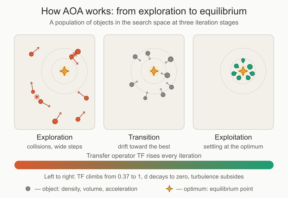
Figure 1. Illustration of how the AOA algorithm works

In the illustration: three panels — the same search space with a fixed optimum (the star represents the equilibrium point) — show the population at three different stages of the process. On the left, exploration — objects are widely scattered, taking long, chaotic steps, with flashes indicating collisions between nearby pairs. In the center, the transition phase — the swarm converges on the best object, with medium-length steps directed inward. On the right is the exploitation phase — a dense cluster near the optimum, with short steps. At the bottom, the TF gradient band (coral → turquoise) connects the stages: it is the same transfer operator that controls the branches in the flow diagram.

Let's write some pseudocode for the AOA algorithm.

INPUT:
  N            — number of objects (Materials_no)
  T_max        — maximum iterations
  dim, lb, ub  — search dimensionality and bounds
  C1 = 2, C2 = 6           — fixed constants
  C3, C4                   — adjustable (usually C3 ∈ {1,2}, C4 ≈ 0.5)
  u = 0.9, l = 0.1         — acceleration normalization range, Eq.(12)

──────────── INITIALIZATION ────────────
for each object i = 1..N:
    X[i]   = lb + rand(dim) · (ub − lb)       // positions,    Eq. (4)
    den[i] = rand(dim)                        // density, Eq. (5)
    vol[i] = rand(dim)                        // volume,      Eq. (5)
    acc[i] = lb + rand(dim) · (ub − lb)       // acceleration, Eq. (6)
    Y[i]   = f(X[i])

(Scorebest, idx) = min(Y)
Xbest = X[idx];  den_best = den[idx];  vol_best = vol[idx];  acc_best = acc[idx]
acc_norm = acc

──────────── MAIN LOOP ────────────
for t = 1..T_max:

    //--- global transition coefficients
    TF = exp((t − T_max) / T_max)             // transfer operator, Eq. (8)
    if TF > 1: TF = 1
    d  = exp((T_max − t)/T_max) − (t/T_max)   // density factor, Eq. (9)

    acc = acc_norm                            // acceleration from the previous iteration
    r   = rand()                              // one number shared across the iteration

    // --- Update density, volume, and acceleration 
    for each object i = 1..N:
        den[i] = den[i] + r · (den_best − den[i])       // Eq. (7)
        vol[i] = vol[i] + r · (vol_best − vol[i])       // Eq. (7)

        if TF ≤ 0.45:                                 // COLLISIONS (exploration)
            mr = random index 1..N
            acc_tmp[i] = (den[mr] + vol[mr]·acc[mr]) /
                         (rand · den[i]·vol[i])         // Eq. (10)
        otherwise:                                      // NO COLLISIONS (exploitation)
            acc_tmp[i] = (den_best + vol_best·acc_best) /
                         (rand · den[i]·vol[i])         // Eq. (11)

    // --- normalize acceleration across the ENTIRE population 
    a_min = min(acc_tmp across all i and j)
    a_max = max(acc_tmp across all i and j)
    for each i, j:
        acc_norm[i,j] = u · (acc_tmp[i,j] − a_min)/(a_max − a_min) + l   // Eq. (12)

    // --- update positions 
    for each object i = 1..N:
        if TF ≤ 0.4:                                 // EXPLORATION
            for each dimension j:
                mrand = random index 1..N
                Xnew[i,j] = X[i,j] + C1·rand·acc_norm[i,j]·
                            (X[mrand,j] − X[i,j])·d              // Eq. (13)
        otherwise:                                         // EXPLOITATION
            for each dimension j:
                p = 2·rand − C4                                  // Eq. (15)
                T = C3 · TF;  if T > 1: T = 1
                if p ≤ 0.5:
                    Xnew[i,j] = Xbest[j] + C2·rand·acc_norm[i,j]·
                                (T·Xbest[j] − X[i,j])·d          // Eq. (14)
                otherwise:
                    Xnew[i,j] = Xbest[j] − C2·rand·acc_norm[i,j]·
                                (T·Xbest[j] − X[i,j])·d

    // --- boundary handling 
    Xnew = clamp(Xnew, lb, ub)

    // --- greedy selection 
    for each object i = 1..N:
        v = f(Xnew[i])
        if v < Y[i]:
            X[i] = Xnew[i];  Y[i] = v

    // --- update the best solution 
    (Ybest, idx) = min(Y)
    if Ybest < Scorebest:
        Scorebest = Ybest
        Xbest = X[idx]
        den_best = den[idx];  vol_best = vol[idx];  acc_best = acc_norm[idx]

OUTPUT: Xbest, Scorebest

Let's move on to examining the implementation of the AOA algorithm.

Class fields. The framework agent (S_AO_Agent) carries only the coordinates (c, cP, cB, cW) and fitness values. But an AOA object requires three more physical attributes — density, volume, and acceleration — and each has its own dynamics. Therefore, they are stored in separate private buffers of the class: den, vol, accNorm, and the intermediate accTemp. All four are flat one-dimensional arrays of size popSize * coords; the element at coordinate c in object i is accessed as [i * coords + c]. A flat layout was chosen over a two-dimensional one for the sake of simplicity and predictable memory access.

Three more buffers of size coords — denBest, volBest, and accBest — store the attributes of the best object; they are needed in Equation (11). The pair snap_c and snap_f represents a snapshot of the population (more on this below). Finally, t and Tmax are the iteration counter and the iteration schedule horizon, respectively. Only two configurable parameters — C3 and C4 — remain public.

The constructor specifies the algorithm's metadata — the AOA name, description, and link to the article — as well as the default values: popSize = 25, C3 = 2.0, C4 = 0.5. Next, the params array is expanded to three elements, and each element stores a parameter's name and value. The test bench uses this array to read and set the algorithm's parameters.

SetParams(). This method reads values from params[] back into the popSize, C3, and C4 fields and applies safeguards: the population size must be at least 2 (the collision phase requires at least one neighbor), and the coefficients C3 and C4 must be nonnegative. SetParams() is called before Init(), so by the time memory is allocated, popSize is already correct.

//+------------------------------------------------------------------+
class C_AO_AOAarch : public C_AO
 {
public:
                    ~C_AO_AOAarch() {}
                     C_AO_AOAarch()
   {
    ao_name = "AOA";
    ao_desc = "Archimedes Optimization Algorithm";
    ao_link = "https://www.mql5.com/en/articles/22648";

    popSize = 25;
    C3      = 2.0;
    C4      = 0.5;

    ArrayResize(params, 3);
    params [0].name = "popSize"; params [0].val  = popSize;
    params [1].name = "C3";      params [1].val  = C3;
    params [2].name = "C4";      params [2].val  = C4;
   }

  void               SetParams()
   {
    popSize = (int)params [0].val;
    C3      = params      [1].val;
    C4      = params      [2].val;

    //--- safeguards
    if(popSize < 2)            // collisions require at least one neighbor
      popSize = 2;
    if(C3 < 0.0)
      C3 = 0.0;
    if(C4 < 0.0)
      C4 = 0.0;
   }

  bool               Init(const double &rangeMinP  [],
                          const double &rangeMaxP  [],
                          const double &rangeStepP [],
                          const int     epochsP = 0);

  void               Moving();
  void               Revision();

  //--- visible parameters
  double             C3;     // scale of the best object's influence: T = C3*TF,   Eq. (15)
  double             C4;     // Step sign offset: p = 2*rand - C4, Eq. (15)

private:
  //--- physical attributes of objects (flat buffers of size popSize*coords)
  double             den     [];   // density,                   Eq. (5), (7)
  double             vol     [];   // volume,                       Eq. (5), (7)
  double             accNorm [];   // acceleration (normalized), Eq. (12)
  double             accTemp [];   // acceleration before normalization,   Eq. (10), (11)

  //--- attributes of the best object (buffers of size coords)
  double             denBest [];
  double             volBest [];
  double             accBest [];

  //--- snapshot for generating candidates and greedy acceptance
  double             snap_c  [];   // popSize * coords
  double             snap_f  [];   // popSize

  //--- iteration schedule
  int                t;            // the number of the current working iteration (1..Tmax)
  int                Tmax;         // total number of working iterations
 };
//+------------------------------------------------------------------+

Init(). Initialization begins with StandardInit() — the base class recreates the array of agents, copies the search ranges, and resets fB and the revision flag. Next come the AOA-specific steps.

First, the schedule is set: Tmax = epochsP - 1. Subtracting one here is crucial — the first epoch of the outer loop is spent on the evaluation of the initial population, leaving epochsP - 1 working iterations, and the TF and d operators must be scheduled over precisely this horizon. The t counter is reset to zero, and Tmax is bounded below by 1.

Next, all buffers are allocated and the initial population state is initialized: coordinates are sampled randomly within the search bounds (Equation 4, stored in cP), density and volume are sampled randomly from [0,1] (Equation 5), and acceleration is sampled randomly within the search bounds (Equation 6). Note: The initial acceleration is written directly to accNorm, rather than to a separate buffer. This is done because, in the first working iteration, the acceleration acc is equal to acc_norm, and there is no point in storing them separately.

//+------------------------------------------------------------------+
//|                              Init                                |
//+------------------------------------------------------------------+
bool C_AO_AOAarch::Init(const double &rangeMinP  [],
                        const double &rangeMaxP  [],
                        const double &rangeStepP [],
                        const int     epochsP = 0)
 {
  if(!StandardInit(rangeMinP, rangeMaxP, rangeStepP))
    return false;

//--- Schedule: The first epoch is spent on the evaluation of the initial population,
//--- therefore, there are epochsP - 1 working iterations
  Tmax = epochsP - 1;
  if(Tmax < 1)
    Tmax = 1;
  t = 0;

//--- buffers
  ArrayResize(den,     popSize * coords);
  ArrayResize(vol,     popSize * coords);
  ArrayResize(accNorm, popSize * coords);
  ArrayResize(accTemp, popSize * coords);
  ArrayResize(denBest, coords);
  ArrayResize(volBest, coords);
  ArrayResize(accBest, coords);
  ArrayResize(snap_c,  popSize * coords);
  ArrayResize(snap_f,  popSize);

//--- initial population and physical attributes
  for(int i = 0; i < popSize; i++)
   {
    for(int c = 0; c < coords; c++)
     {
      //--- positions, Eq. (4) — stored in cP[], transferred to c[] on the first call to Moving
      a [i].cP [c] = u.RNDfromCI(rangeMin [c], rangeMax [c]);

      //--- density and volume ~ U[0,1], Eq. (5)
      den [i * coords + c] = u.RNDfromCI(0.0, 1.0);
      vol [i * coords + c] = u.RNDfromCI(0.0, 1.0);

      //--- acceleration ~ U[lb,ub], Eq. (6).
      //--- store in accNorm: on the first iteration, acc = acc_norm = this value
      accNorm [i * coords + c] = u.RNDfromCI(rangeMin [c], rangeMax [c]);
     }
   }

  return true;
 }
//+------------------------------------------------------------------+

Moving(). This is the heart of the algorithm. The first call is special: while revision is 'false', the method simply transfers the initial coordinates from cP to c (using u.SeInDiSp to snap them to the grid and keep them within bounds) and exits. This allows the outer loop to evaluate the initial population.

On subsequent calls, the algorithm constants are first set: C1 = 2, C2 = 6, the normalization limits uN = 0.9 and lN = 0.1, the phase thresholds TFc = 0.45 and TFx = 0.40, and EPS to safeguard denominators. The iteration then proceeds in stages.

Stage 0 — snapshot. The coordinates and fitness values of all agents are copied to snap_c and snap_f. We need the snapshot for two reasons. First, equations (13) and (14) read the positions at the start of the iteration, while the method immediately overwrites a[i].c with new candidates — without a snapshot, an agent processed earlier would distort the input for one processed later. Second, the snapshot is the basis for the greedy selection in Revision().

Step 1 — Schedule. The counter t is incremented, and the transfer operator TF (Formula 8, capped at 1), the density factor d (Formula 9), and the random number r (Formula 7), which is shared across the iteration, are calculated.

Step 2 — Attributes. In a single loop over the agents, the density and volume are first updated — they move toward the best object's values in-place (Equation 7) — and then the raw acceleration, accTemp, is calculated. If TF is below the threshold TFc, this is the collisions phase: a random object mr is selected, and its acceleration is used (Equation 10). Otherwise, in the phase without collisions, the acceleration is taken from the best object (Equation 11). Updating den/vol in-place means that the object with the lower index has already been updated by the time the object with the higher index reads it — this intentionally mirrors the order of the reference code. The EPS check in the denominator prevents inf or nan results if the density, volume, or random factor is zero.

Step 3 — Normalization. Global minimum and maximum values are determined across the entire accTemp buffer (all objects, all coordinates), and the acceleration is linearly mapped to the interval [lN, uN] (Equation 12); the result is stored in accNorm. The degenerate case where all accelerations are equal is handled separately.

Step 4 — Positions. The factor T = C3 · TF, capped at 1, is calculated (Formula 15). Then, for each agent: if TF is below TFx, the exploration phase applies, with a step toward a random object (Formula 13); otherwise, the exploitation phase applies, with a step relative to the global best cB, and the sign of the step in each coordinate is determined by the value p (Formulas 14–15). All new coordinates are passed through u.SeInDiSp, which handles boundaries and enforces the grid step size for each coordinate, replacing the flawed fun_checkpositions check in the original code.

//+----------------------------------------------------------------------+
//|                            Moving                                    |
//|                                                                      |
//|  Structure of a working iteration:                                   |
//|    0. Snapshot of the current population;                            |
//|    1. the transition coefficients TF (Eq. 8) and d (Eq. 9);          |
//|    2. Update den/vol (Eq. 7) + calculate accTemp:                    |
//|         TF < 0.45 — collisions, Eq. (10);                            |
//|         otherwise      — no collisions, Eq. (11);                    |
//|    3. Normalize acceleration across the entire population, Eq. (12); |
//|    4. Update positions:                                              |
//|         TF < 0.4  — exploration, Eq. (13);                           |
//|         otherwise      — exploitation, Eqs. (14)–(15).               |
//+----------------------------------------------------------------------+
void C_AO_AOAarch::Moving()
 {
//--- First run: cP → c for the evaluation of the initial population
  if(!revision)
   {
    for(int i = 0; i < popSize; i++)
      for(int c = 0; c < coords; c++)
        a [i].c [c] = u.SeInDiSp(a [i].cP [c],
                                 rangeMin  [c],
                                 rangeMax  [c],
                                 rangeStep [c]);
    return;
   }

//--- algorithm constants (Hashim et al., 2021)
  const double C1   = 2.0;     // exploration step scaling factor,       Eq. (13)
  const double C2   = 6.0;     // exploitation step scaling factor,   Eq. (14)
  const double uN   = 0.9;     // upper normalization bound, Eq. (12)
  const double lN   = 0.1;     // lower normalization bound, Eq. (12)
  const double TFc  = 0.45;    // collision phase threshold
  const double TFx  = 0.40;    // threshold for the position exploration phase
  const double EPS  = 1e-300;  // denominator safeguards against inf/nan

//--- 0. snapshot
  for(int i = 0; i < popSize; i++)
   {
    for(int c = 0; c < coords; c++)
      snap_c [i * coords + c] = a [i].c [c];
    snap_f [i] = a [i].f;
   }

//--- 1. Transition coefficients
  t++;
  double tt = 1; //(double)t;
  double Tm = (double)Tmax;

  double TF = MathExp((tt - Tm) / Tm);              // transfer operator, Eq. (8)
  if(TF > 1.0)
    TF = 1.0;

  double d  = MathExp((Tm - tt) / Tm) - (tt / Tm);  // density factor, Eq. (9)

  double r  = u.RNDfromCI(0.0, 1.0);                // shared across the iteration, Eq. (7)

//--- 2. Update den/vol + calculate accTemp
  for(int i = 0; i < popSize; i++)
   {
    //--- density and volume move toward the best object's values (in-place), Eq. (7)
    for(int c = 0; c < coords; c++)
     {
      int idx = i * coords + c;
      den [idx] += r * (denBest [c] - den [idx]);
      vol [idx] += r * (volBest [c] - vol [idx]);
     }

    double rnd = u.RNDfromCI(0.0, 1.0);             // a fresh scalar for each object

    if(TF < TFc)
     {
      //--- COLLISION PHASE (exploration), Eq. (10)
      int mr = (int)u.RNDfromCI(0.0, (double)popSize);
      if(mr >= popSize)
        mr = popSize - 1;
      if(mr < 0)
        mr = 0;

      for(int c = 0; c < coords; c++)
       {
        int idx  = i  * coords + c;
        int idxR = mr * coords + c;

        double denom = rnd * den [idx] * vol [idx];
        if(MathAbs(denom) < EPS)
          denom = (denom < 0.0 ? -EPS : EPS);

        accTemp [idx] = (den [idxR] + vol [idxR] * accNorm [idxR]) / denom;
       }
     }
    else
     {
      //--- NO COLLISIONS (exploitation), Eq. (11)
      for(int c = 0; c < coords; c++)
       {
        int idx = i * coords + c;

        double denom = rnd * den [idx] * vol [idx];
        if(MathAbs(denom) < EPS)
          denom = (denom < 0.0 ? -EPS : EPS);

        accTemp [idx] = (denBest [c] + volBest [c] * accBest [c]) / denom;
       }
     }
   }

//--- 3. Normalization of acceleration across the entire population, Eq. (12)
  int    total = popSize * coords;
  double gMin  = accTemp [0];
  double gMax  = accTemp [0];

  for(int k = 1; k < total; k++)
   {
    double v = accTemp [k];
    if(v < gMin)
      gMin = v;
    if(v > gMax)
      gMax = v;
   }

  double span = gMax - gMin;

  for(int k = 0; k < total; k++)
   {
    if(span > EPS)
      accNorm [k] = uN * (accTemp [k] - gMin) / span + lN;
    else
      accNorm [k] = lN;     // a degenerate case: all accelerations are equal
   }

//--- 4. Update positions
  double T = C3 * TF;                               // Eq. (15)
  if(T > 1.0)
    T = 1.0;

  for(int i = 0; i < popSize; i++)
   {
    if(TF < TFx)
     {

      //--- EXPLORATION PHASE, Eq. (13)
      for(int c = 0; c < coords; c++)
       {
        int mrand = (int)u.RNDfromCI(0.0, (double)popSize);
        if(mrand >= popSize)
          mrand = popSize - 1;
        if(mrand < 0)
          mrand = 0;

        int    idx   = i * coords + c;
        double x_old = snap_c [idx];
        double x_rnd = snap_c [mrand * coords + c];

        double v = x_old + C1 * u.RNDfromCI(0.0, 1.0) * accNorm [idx] *
                   (x_rnd - x_old) * d;

        a [i].c [c] = u.SeInDiSp(v, rangeMin [c], rangeMax [c], rangeStep [c]);
       }
     }
    else
     {
      //--- EXPLOITATION PHASE, Eq. (14)
      for(int c = 0; c < coords; c++)
       {
        int    idx  = i * coords + c;
        double p    = 2.0 * u.RNDfromCI(0.0, 1.0) - C4;    // Eq. (15)

        double step = C2 * u.RNDfromCI(0.0, 1.0) * accNorm [idx] *
                      (T * cB [c] - snap_c [idx]) * d;

        double v;
        if(p < 0.5)
          v = cB [c] + step;
        else
          v = cB [c] - step;

        a [i].c [c] = u.SeInDiSp(v, rangeMin [c], rangeMax [c], rangeStep [c]);
       }
     }
   }
 }
//+------------------------------------------------------------------+

Revision(). This method completes the iteration. The first call is special again: the initial population has just been evaluated, so the method updates the agents’ personal bests and the global fB / cB, saves the index of the best object, and copies its attributes to denBest, volBest, and accBest, then sets revision = true and exits. There's no greedy selection here — the snapshot does not exist yet.

On subsequent calls, greedy selection is performed first: if the agent's new fitness is worse than the value in the snapshot, its coordinates and fitness are restored from snap_c / snap_f. It is important to note that the attributes den, vol, and acc are not subject to rollback — they evolve independently. After selection, the personal and global bests are updated, and if the global best has improved, the den / vol / accNorm values from the new best object are copied into the buffers for the best object. The order — selection first, then choosing the best — matches the reference implementation: the best object is chosen from the accepted population.

//+-------------------------------------------------------------------------------+
//|                           Revision                                            |
//|                                                                               |
//|  Greedy acceptance: the agent's position/fitness is restored from             |
//|  the snapshot if the new candidate turns out to be worse. Attributes          |
//|  den/vol/acc are NOT subject to rollback—they evolve independently.           |
//|  Next, the best solutions and the attributes of the best object are updated.  |
//+-------------------------------------------------------------------------------+
void C_AO_AOAarch::Revision()
 {
//--- first run: evaluation of the initial population, selection of the best object
  if(!revision)
   {
    int bestIdx = -1;

    for(int i = 0; i < popSize; i++)
     {
      if(a [i].f > a [i].fB)
       {
        a [i].fB = a [i].f;
        ArrayCopy(a [i].cB, a [i].c, 0, 0, coords);
       }
      if(a [i].f > fB)
       {
        fB = a [i].f;
        ArrayCopy(cB, a [i].c, 0, 0, coords);
        bestIdx = i;
       }
     }

    //--- attributes of the best object in the initial population
    if(bestIdx >= 0)
     {
      for(int c = 0; c < coords; c++)
       {
        denBest [c] = den     [bestIdx * coords + c];
        volBest [c] = vol     [bestIdx * coords + c];
        accBest [c] = accNorm [bestIdx * coords + c]; // raw acceleration, Eq. (6)
       }
     }

    revision = true;
    return;
   }

//--- greedy acceptance: roll back if the result is worse
  for(int i = 0; i < popSize; i++)
   {
    if(a [i].f < snap_f [i])
     {
      for(int c = 0; c < coords; c++)
        a [i].c [c] = snap_c [i * coords + c];
      a [i].f = snap_f [i];
     }
   }

//--- update personal/global bests + capture the best object's attributes
  int bestIdx = -1;

  for(int i = 0; i < popSize; i++)
   {
    if(a [i].f > a [i].fB)
     {
      a [i].fB = a [i].f;
      ArrayCopy(a [i].cB, a [i].c, 0, 0, coords);
     }
    if(a [i].f > fB)
     {
      fB = a [i].f;
      ArrayCopy(cB, a [i].c, 0, 0, coords);
      bestIdx = i;
     }
   }

//--- the best object's den/vol/acc values are updated only when the global best improves
  if(bestIdx >= 0)
   {
    for(int c = 0; c < coords; c++)
     {
      denBest [c] = den     [bestIdx * coords + c];
      volBest [c] = vol     [bestIdx * coords + c];
      accBest [c] = accNorm [bestIdx * coords + c];
     }
   }
 }
//+------------------------------------------------------------------+

Test Results

An AOA run on the standard test bench yields an overall result of 39.66%. Unfortunately, that is not enough to make it onto the leaderboard. But what is more interesting is not the number itself, but the results that make it up; more on this in the conclusions.

AOA|Archimedes Optimization Algorithm|25.0|2.0|0.5|
=============================
5 Hilly's; Func runs: 10000; result: 0.8206488162634686
25 Hilly's; Func runs: 10000; result: 0.4924635010346886
500 Hilly's; Func runs: 10000; result: 0.2768438671570971
=============================
5 Forest's; Func runs: 10000; result: 0.6788879303684001
25 Forest's; Func runs: 10000; result: 0.24788382890806288
500 Forest's; Func runs: 10000; result: 0.06499823135837557
=============================
5 Megacity's; Func runs: 10000; result: 0.5906666666666667
25 Megacity's; Func runs: 10000; result: 0.27759999999999996
500 Megacity's; Func runs: 10000; result: 0.11920000000000104
=============================
All score: 3.56919 (39.66%)

The anti-cheat test shows a similar pattern to the scores for the first functions in the preceding main test. An honest algorithm.

AOA|Archimedes Optimization Algorithm|25.0|2.0|0.5|
=============================
Composite anti-cheat test: Hilly + Forest + Megacity + Peaks + Skin
Coordinates: 10; Epochs: 400; Repeats: 10
=============================
Run 1/10: 0.6677793808019812
Run 2/10: 0.6355386750189551
Run 3/10: 0.5813048402935594
Run 4/10: 0.7378557003396822
Run 5/10: 0.7012834397505456
Run 6/10: 0.6202804626691847
Run 7/10: 0.8256544601079605
Run 8/10: 0.7089113881121764
Run 9/10: 0.9011830945159774
Run 10/10: 0.9514789578735151
=============================
Average result: 0.7331270399 (73.31%)
=============================

A visualization of how the algorithm works on our first three test functions and, additionally, on a few others.

AOA on the Hilly test function

AOA on the Forest test function

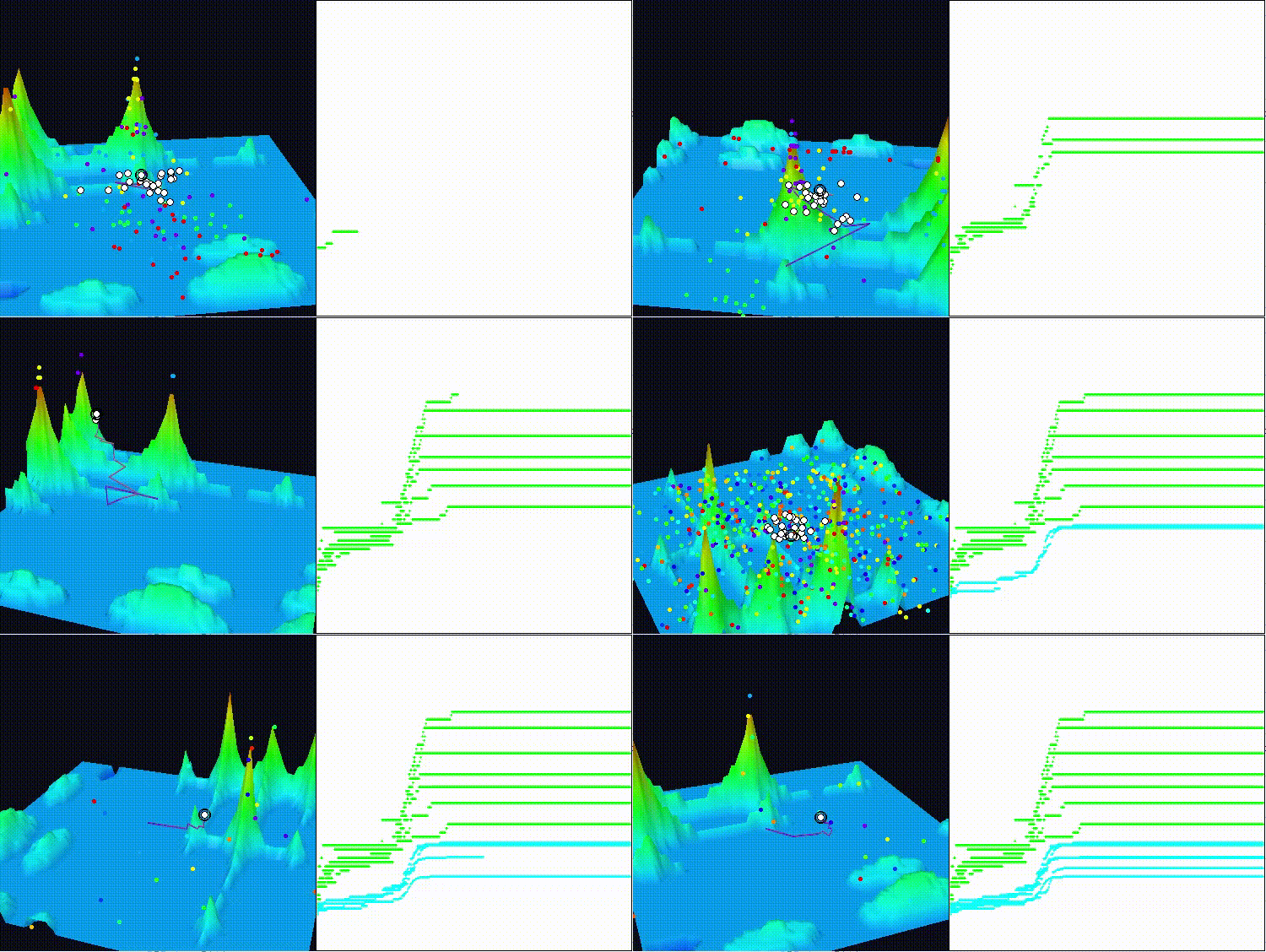
AOA on the Megacity test function

AOA on the Rosenbrock function

AOA on the Ackley function

Based on the test results, the AOA algorithm is presented in the ranking table for informational purposes.

cc	AO	Description	Hilly			Hilly Final	Forest			Forest Final	Megacity (discrete)			Megacity Final	Final Result	% of MAX
			10 p (5 F)	50 p (25 F)	1,000 p (500 F)		10 p (5 F)	50 p (25 F)	1,000 p (500 F)		10 p (5 F)	50 p (25 F)	1,000 p (500 F)
1	ANS	across neighbourhood search	1.00000	0.88228	0.40138	2.28366	1.00000	0.95281	0.28092	2.23373	0.94667	0.85733	0.22389	2.02789	6.545	72.72
2	AMOm	animal migration optimization M	0.91624	0.83603	0.46790	2.22017	0.98482	0.92010	0.36391	2.26883	0.91733	0.81707	0.25177	1.98617	6.475	71.94
3	CLA	code lock algorithm (joo)	0.95139	0.86199	0.37879	2.19217	0.99349	0.93500	0.26497	2.19346	0.93600	0.84267	0.24060	2.01927	6.405	71.17
4	(P+O)ES	(P+O) evolution strategies	0.86571	0.89539	0.39740	2.15850	0.97761	0.89820	0.26878	2.14459	0.92133	0.80240	0.23952	1.96325	6.266	69.62
5	SDSm	stochastic diffusion search M	0.95195	0.84944	0.36249	2.16388	0.98061	0.88457	0.22112	2.08630	0.92267	0.79013	0.21380	1.92660	6.177	68.63
6	AAm	archery algorithm M	0.84685	0.73320	0.42590	2.00595	0.96709	0.77837	0.27789	2.02335	0.86133	0.77707	0.28712	1.92552	5.955	66.17
7	SIA	simulated isotropic annealing (joo)	0.93543	0.86504	0.38483	2.18530	0.94069	0.80609	0.23835	1.98513	0.86400	0.66160	0.19536	1.72096	5.891	65.46
8	TETA	time evolution travel algorithm (joo)	0.91452	0.86369	0.25579	2.03400	0.99654	0.91291	0.14394	2.05339	0.85467	0.82213	0.10443	1.78123	5.869	65.21
9	ESG	evolution of social groups (joo)	0.98111	0.79857	0.31167	2.09135	0.98954	0.82270	0.15032	1.96256	0.92133	0.73440	0.15315	1.80888	5.863	65.14
10	CTA	comet tail algorithm (joo)	0.92435	0.86786	0.27838	2.07059	0.99039	0.84571	0.19448	2.03058	0.95467	0.69680	0.11008	1.76155	5.863	65.14
11	ECBO	enhanced colliding bodies optimization	0.94024	0.72363	0.32356	1.98743	0.99477	0.80291	0.13056	1.92824	0.87600	0.70160	0.17433	1.75193	5.668	62.98
12	DA	dialectical algorithm	0.93117	0.75400	0.26205	1.94722	0.98925	0.81375	0.08662	1.88962	0.92667	0.68107	0.11315	1.72089	5.558	61.76
13	BBO	biogeography-based optimization	0.95876	0.70609	0.35752	2.02237	0.92981	0.70660	0.16970	1.80611	0.87467	0.63013	0.20813	1.71293	5.541	61.57
14	BHAm	black hole algorithm M	0.79558	0.76207	0.34682	1.90447	0.99836	0.75798	0.13826	1.89460	0.85067	0.64427	0.17020	1.66514	5.464	60.71
15	HS	harmony search	0.91420	0.69049	0.29924	1.90393	0.97627	0.73373	0.14193	1.85193	0.91733	0.62720	0.15364	1.69817	5.454	60.60
16	RFO	royal flush optimization (joo)	0.80989	0.74481	0.34546	1.90016	0.95251	0.77926	0.15185	1.88362	0.80400	0.66427	0.19071	1.65898	5.443	60.48
17	BOAm	billiards optimization algorithm M	0.76177	0.72421	0.25275	1.73873	0.90890	0.81960	0.28853	2.01703	0.83733	0.74613	0.09763	1.68109	5.437	60.41
18	ASO	anarchy society optimization	0.73070	0.73713	0.31195	1.77978	0.99732	0.87700	0.17619	2.05051	0.72000	0.68773	0.18988	1.59761	5.428	60.31
19	EOm	extremal optimization_M	0.76527	0.75205	0.31908	1.83640	0.99999	0.76426	0.12437	1.88862	0.84133	0.64133	0.15247	1.63513	5.360	59.56
20	ACS	artificial cooperative search	0.75545	0.77162	0.31653	1.84360	1.00000	0.80488	0.10705	1.91193	0.76933	0.60800	0.14157	1.51890	5.274	58.60
21	SSG	saplings sowing and growing	0.75436	0.63206	0.35935	1.74577	0.91907	0.69694	0.19755	1.81356	0.81867	0.60533	0.21347	1.63747	5.197	57.74
22	AOSm	atomic orbital search M	0.76184	0.68435	0.31344	1.75963	0.90015	0.80044	0.11501	1.81560	0.82800	0.63280	0.15696	1.61776	5.193	57.70
23	TSEA	turtle shell evolution algorithm (joo)	0.95809	0.64852	0.29571	1.90232	0.99522	0.58104	0.10542	1.68168	0.92133	0.52160	0.14567	1.58860	5.173	57.48
24	DE	differential evolution	0.96398	0.62346	0.26089	1.84833	0.98482	0.77018	0.11459	1.86959	0.93067	0.36213	0.11000	1.40280	5.121	56.90
25	BIO	blood inheritance optimization (joo)	0.72580	0.66522	0.31228	1.70330	0.99995	0.68125	0.11540	1.79660	0.85467	0.59333	0.15364	1.60164	5.102	56.69
26	(PO)ES	(PO) evolution strategies	0.73972	0.58190	0.38896	1.71058	0.91199	0.59975	0.21262	1.72436	0.82400	0.56240	0.23432	1.62072	5.056	56.18
27	BO	bonobo optimizer	0.75555	0.64366	0.32657	1.72578	0.94332	0.70442	0.13999	1.78773	0.73467	0.61440	0.16728	1.51635	5.030	55.89
28	SRA	successful restaurateur algorithm (joo)	0.89010	0.63359	0.29115	1.81484	0.96634	0.55285	0.08914	1.60833	0.89333	0.52800	0.13911	1.56044	4.984	55.38
29	CRO	chemical reaction optimisation	0.91281	0.65681	0.29866	1.86828	0.90513	0.56020	0.10939	1.57472	0.82800	0.50133	0.14149	1.47082	4.914	54.60
30	BCOm	bacterial chemotaxis optimization M	0.82589	0.61733	0.31584	1.75906	0.95296	0.63718	0.11984	1.70998	0.76533	0.51653	0.15800	1.43986	4.909	54.54
31	DOA	dream optimization algorithm	0.78522	0.78121	0.36036	1.92679	0.61584	0.42117	0.12254	1.15955	0.86667	0.72587	0.21127	1.80381	4.890	54.33
32	ABO	african buffalo optimization	0.92295	0.62528	0.29885	1.84708	0.92992	0.57468	0.09372	1.59832	0.73333	0.51333	0.14324	1.38990	4.835	53.72
33	BSA	bird swarm algorithm	0.94432	0.67941	0.26401	1.88774	0.91649	0.65619	0.12054	1.69322	0.80933	0.33547	0.10652	1.25132	4.832	53.69
34	TSm	tabu search M	0.87806	0.61040	0.28993	1.77839	0.98116	0.52165	0.08544	1.58825	0.82667	0.49547	0.13552	1.45766	4.824	53.60
35	BSA	backtracking search algorithm	0.87128	0.53190	0.28675	1.68993	0.92408	0.51602	0.09153	1.53163	0.96000	0.47253	0.13760	1.57013	4.792	53.24
36	WOAm	whale optimization algorithm M	0.93893	0.59477	0.26695	1.80065	0.98036	0.53873	0.07112	1.59021	0.78667	0.47600	0.11892	1.38159	4.772	53.02
37	ACA	andean_condor_algorithm	0.78444	0.53260	0.33108	1.64812	0.79071	0.44960	0.10685	1.34716	0.92266	0.67733	0.17613	1.77612	4.771	53.02
38	CSO	competitive swarm optimizer	0.85151	0.60786	0.29896	1.75833	0.84085	0.58491	0.11974	1.54550	0.80000	0.48560	0.14184	1.42744	4.731	52.57
39	FBA	fractal-based algorithm	0.69419	0.64267	0.28955	1.62641	0.99812	0.54905	0.08705	1.63422	0.76133	0.51253	0.13689	1.41075	4.671	51.90
40	ECOi	eco-inspired evolutionary algorithm	0.78817	0.54402	0.29360	1.62579	0.88996	0.46592	0.09747	1.45335	0.78533	0.45173	0.14295	1.38001	4.459	49.54
41	BSO	brain storm optimization	0.92207	0.57625	0.29732	1.79564	0.80764	0.42508	0.09448	1.32720	0.77200	0.36533	0.13065	1.26798	4.391	48.79
42	CAm	camel algorithm M	0.71534	0.56917	0.35985	1.64436	0.84094	0.47174	0.10850	1.42118	0.70400	0.41947	0.19563	1.31910	4.385	48.72
43	ACOm	ant colony optimization_M	0.71885	0.48410	0.30990	1.51285	0.75792	0.48639	0.11871	1.36302	0.83600	0.48667	0.16148	1.48415	4.360	48.44
44	BSO	brain storm optimization	0.91331	0.55813	0.29705	1.76849	0.85329	0.44038	0.09447	1.38814	0.72267	0.32880	0.13325	1.18472	4.341	48.23
45	AEFA	artificial electric field algorithm	0.88798	0.65769	0.25276	1.79843	0.95550	0.63602	0.03946	1.63098	0.60800	0.16000	0.09845	0.86645	4.296	47.73
	AOA	archimedes_optimization_algorithm	0.82064	0.49246	0.27684	1.58994	0.67888	0.24788	0.06500	0.99176	0.59066	0.27759	0.11920	0.98745	3.569	39.66
	RW	random walk	0.49970	0.32333	0.25791	1.08094	0.30754	0.11470	0.04400	0.46624	0.36133	0.17013	0.10244	0.63390	2.181	24.23

Conclusions

Running AOA on the standard test bench yielded an overall score of 39.66%. That wasn't enough to make it into the rankings — the algorithm remains outside the group of leaders that have already been analyzed. But what is more interesting is not the number itself, but how it breaks down.

Let's look at the results by dimensionality. On average across the three functions, AOA achieves about 70% on problems with 10 coordinates, about 34% on problems with 50, and only about 15% on problems with 1,000. With each increase in dimensionality, the score drops by roughly half. This is most evident on Forest: 68% → 25% → 6.5%. The pattern is the same across all three landscapes — Hilly, Forest, and Megacity — so this is a consistent trend, not random variation.

This profile is a characteristic sign of premature convergence. For low-dimensional problems, AOA performs quite well: the space is compact, there is nowhere to get lost, and the algorithm carefully finds a good region. But the more coordinates there are, the sooner the population collapses. At this point, it is worth revisiting the structure of the algorithm. Exploration is enabled in AOA only while TF is small, and the thresholds (0.45 and 0.4) restrict this phase to roughly the first 8–20% of iterations; after that, it is all exploitation, moving toward the best object. In a five-dimensional problem, this is sufficient. In a 500-dimensional problem, it is not: the turbulence subsides before the swarm has time to explore the space, and the objects settle near the first decent optimum found by chance early on. The liquid comes to rest too soon — and freezes in the wrong place.

A composite anti-cheat test confirms that the numbers can be trusted. Across five functions with differently shaped optima, AOA scored 73.31%, which is consistent with its genuine strength at low dimensionalities — each function in the composite receives only a two-dimensional slice. If AOA relied on a geometric cheat such as diagonal alignment, the composite would have sent its score plummeting; that didn't happen. In other words, both the strength and the weakness are genuine — not artifacts.

In terms of stability, AOA is a solid middle-of-the-pack performer. The variation between runs is noticeable but not erratic: the algorithm does not produce consistently high or consistently low results — it falls within a wide but predictable range. In practice, this means that you should not rely on a single run; you need to average the results of several runs.

And yet, I am reluctant to write AOA off as a failure. The idea — to redefine optimization as the search for equilibrium and to leave the exploration/exploitation balance to physics — is both elegant and workable; it proves effective at low dimensionalities. The weak point is not the model itself, but its default configuration, which was inherited from the reference article: the schedule is skewed toward exploitation. The obvious path to improvement is exactly the one we identified during implementation: expose the phase thresholds as parameters and adjust them to extend exploration, and perhaps make the proportion of exploration depend on the problem's dimensionality. With this reworking, AOA could well achieve a score significantly higher than its current 39.66%.

All the tools — the C_AO_AOA class, the standard test bench, and the composite anti-cheat test — are right at the reader's fingertips. I invite you not to stop at these conclusions, but to test them out and do your own research: perhaps someone will have more success than I did. AOA in its current form is not the final answer, but an open problem.

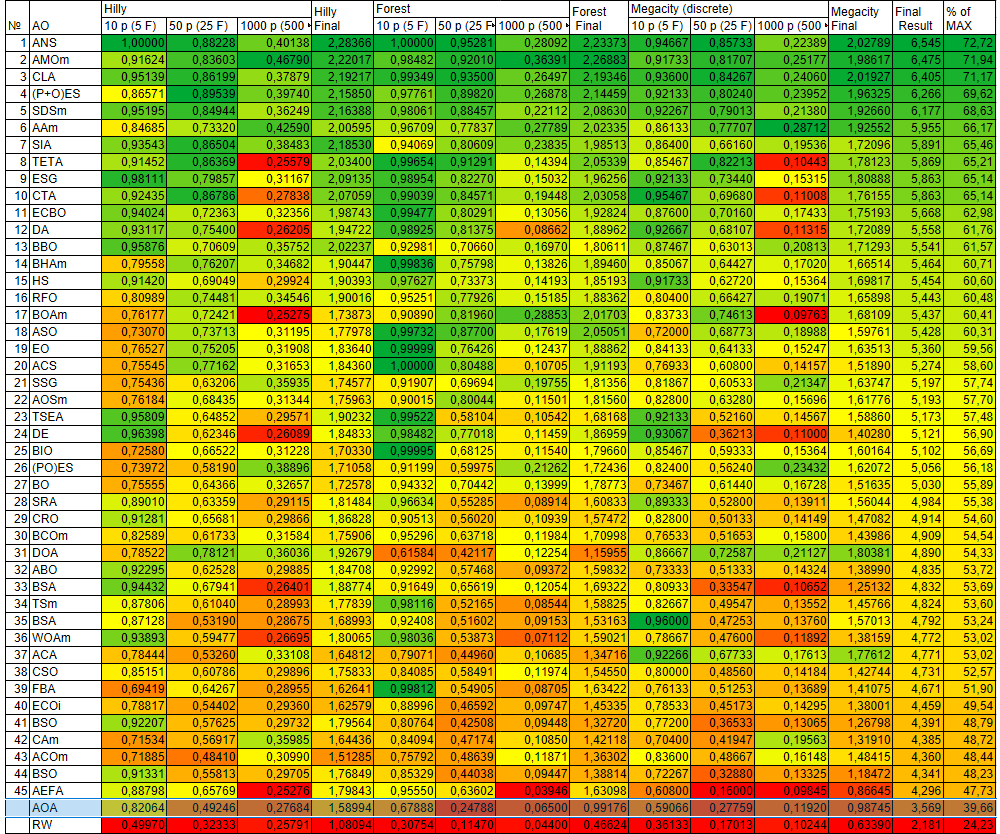
Figure 2. Color gradation of algorithms by their results on the corresponding tests

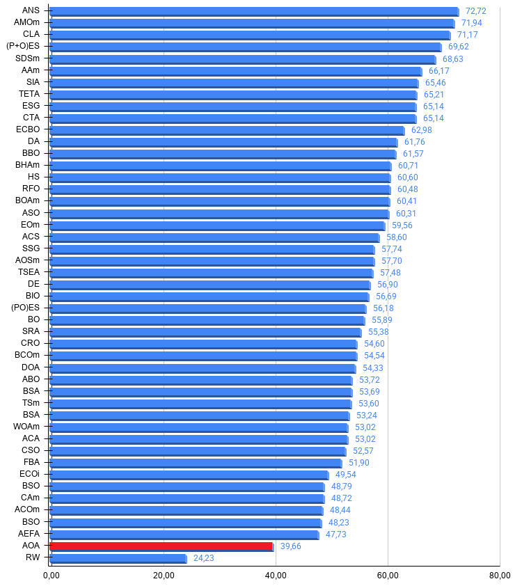
Figure 3. A histogram of the algorithm test results (on a scale from 0 to 100; the higher the score, the better, where 100 is the maximum possible theoretical result); the archive contains a script for calculating the ranking table

Pros and Cons of the Algorithm

Pros:

1. A small number of external parameters.

Cons:

1. Tendency to get stuck.
2. The internal parameters require tuning.

An archive containing the latest versions of the algorithms' source code is attached to the article. The author of this article does not guarantee complete accuracy in the descriptions of canonical algorithms; many of them have been modified to improve their search capabilities. The conclusions and judgments presented in the articles are based on the results of the experiments conducted.

• GitHub: https://github.com/JQSakaJoo/Population-optimization-algorithms-MQL5

Programs used in this article

#	Name	Type	Description
1	#C_AO.mqh	Include file	Parent class for population-based optimization algorithms
2	#C_AO_enum.mqh	Include file	Enumeration of population-based optimization algorithms
3	TestFunctions.mqh	Include file	Test function library
4	TestStandFunctions.mqh	Include file	Test bench function library
5	TestStand3D.mqh	Include file	3D visualization panel for a test bench
6	Utilities.mqh	Include file	Utility functions library
7	CalculationTestResults.mqh	Include file	Script for calculating results for the comparison table
8	Test_AO_All.mq5	Script	Unified test bench for all population-based optimization algorithms
9	Test_AO_AntiCheat	Script	Test for cheating in optimization algorithms
10	Simple use of population optimization algorithms.mq5	Script	Simple example of using population-based optimization algorithms without visualization
11	Test_AO_AOA.mq5	Script	Test bench for AOA