

Buzzard Optimization Algorithm (BUZOA)
 410
 0

Table of Contents
Introduction
Among population-based optimization algorithms, particle swarm optimization (PSO) is a method on which most modern hybrid algorithms are based. The basic PSO scheme has been known for decades; its strengths and weaknesses have been studied, and attempts to improve it generally move in one direction: making the mathematics more complex, adding adaptive coefficients, and introducing new operators. But what if we look at the problem from a different angle — not by making the equations more complex, but by changing the agent's decision-making logic itself? What if, at every moment in time, each particle randomly chooses one of several qualitatively different behavioral strategies, just as living beings do in nature? This is precisely the approach devised by the authors of BUZOA, and the question is whether this biologically motivated mode switching actually offers something that classical PSO-like algorithms do not — or whether it is merely an attractive metaphor with no practical value.
The reader will get a fully analyzed metaheuristic BUZOA algorithm, implemented in MQL5 and tested as part of our test bench, with a detailed analysis of its three hunting modes, a comparison of the literal formulas from the article by Arshagi, Ashurian, and Gabeli (2019) with their rational interpretation, a benchmark on the Hilly, Forest, and Megacity test functions, and recommendations for parameter tuning. At the same time, the reader will see how a biological analogy — sight, smell, and tracking predators — is translated into the mathematical language of velocity, inertia, and random scattering, and will be able to assess how well this analogy works in practice.
Algorithm Implementation
Vultures are among the few animals that have developed a collective foraging strategy based on two independent channels of information: smell and sight. Turkey vultures (Cathartes aura) have an exceptionally keen sense of smell and can detect carrion from a distance of more than a kilometer. Black vultures (Coragyps atratus) have virtually no sense of smell, but they compensate for this with keen eyesight: rather than searching for food directly, they observe the behavior of turkey vultures from above. As soon as the turkey vulture descends, the black vultures dive in after it and often drive away the discoverer.
In addition to these two scenarios, vultures sometimes discover a food source in a completely different way: by spotting, from a great height, a group of terrestrial predators (wolves, dogs) gathered around prey and immediately flying in to that location from all around. It is precisely these three biological scenarios that form the basis of the BUZOA algorithm.
Each agent in the population represents a single vulture, characterized by two vectors. The first is the position vector L, which specifies the bird's current location in the search space. The second is the ability vector C, which — similar to velocity in the Particle Swarm Optimization (PSO) method — determines how far and in which direction an agent will move in the next step. This division allows the movement to maintain its “accumulated momentum”: the vulture does not stop abruptly, but smoothly changes its trajectory in response to new information.
Each agent remembers the best position it has ever occupied (its personal best, pBest), and the entire flock knows the best position found globally (global best, gBest). The ability vector is restricted to the range [−C_max, +C_max], where C_max = (L_max − L_min) / 2; that is, it does not exceed half the width of the search space in each dimension. This prevents agents from accelerating uncontrollably and keeps them within reasonable limits.
Initialization. At the start of the run, each agent is assigned a random position, uniformly distributed throughout the search space, and a random initial ability from the range [−C_max, +C_max]. This initialization ensures maximum initial diversity in the population.
Let's consider a simple example in one-dimensional space on the interval [0, 100]. Let C_max = 50. Agent A was assigned an initial position of L = 30 and an initial ability of C = +12, while Agent B was assigned a position of L = 70 and an ability of C = −8. Without any update, Agent A would shift toward higher coordinate values, and Agent B toward lower coordinate values.
Three hunting modes. At each iteration, a uniformly distributed random number in the range [0, 1] is generated independently for each agent, determining which of the three scenarios the agent will follow in the current step. All three modes are active simultaneously in different parts of the population, which creates a balance between convergence and diversity.
Mode 001 — exploitation. In this mode, the vulture hunts on its own, without relying on its neighbors. Its only reference point is its own personal best, pBest. The ability update is described by the equation:
C(t) = α₁ · C(t−1) + c1 · r · (pBest − L)
The first term, α₁ · C(t−1), preserves the inertia of the previous motion: if the bird was flying to the right, it will continue to fly to the right, but slightly slower (α₁ < 1). The second term pulls the agent toward its personal best: the difference (pBest − L) indicates how far away and in which direction the best-known position lies, while the random factor r ∈ [0, 1] gives this attraction a stochastic nature.
For example, an agent with L = 30, C = +12, and pBest = 45, given α₁ = 0.75, c1 = 1.5, and r = 0.6, will obtain a new ability value of C = 0.75 · 12 + 1.5 · 0.6 · (45 − 30) = 9 + 13.5 = 22.5. After applying the C_max = 50 limit, the value will not change, and the new position will be L = 30 + 22.5 = 52.5. The agent moves rapidly toward its personal best.
Mode 010 — scent-based exploration. This mode simulates the behavior of a flock led by a turkey vulture. The calculation is performed in two steps. First, the base ability C₁ is calculated using the same formula as in mode 001: the agent accounts for inertia and the pull toward its personal best. Then, two additional terms are added to C₁:
C(t) = C₁ + c1 · r₁ · (pBest − L) + c2 · r₂ · (gBest − L)
The first additional component is a repeated cognitive attraction to pBest; the second is a social attraction to the global best, gBest. Both terms are written in terms of position differences, which ensures dimensional consistency: velocity is formed from coordinate differences rather than from heterogeneous quantities.
Let's continue with the example. Let the agent have L = 30, C₁ = 22.5 (from the previous step), pBest = 45, gBest = 80, r₁ = 0.4, and r₂ = 0.7. Then C = 22.5 + 1.5 · 0.4 · (45 − 30) + 1.5 · 0.7 · (80 − 30) = 22.5 + 9 + 52.5 = 84. After clipping at C_max = 50, we get C = 50, and the new position is L = 30 + 50 = 80. The agent is pulled sharply toward the global leader — this is precisely the behavior that describes pursuit of detected carrion.
Mode 010 is the most powerful from an exploration perspective: simultaneous attraction toward pBest and gBest can pull the agent far away from its current position, which is particularly valuable at the beginning of optimization, when the population has not yet concentrated.
Mode 100 — Global Dispersal. This mode simulates the behavior of a black vulture that has spotted a cluster of predators in a completely different area. The agent leaves its current location and immediately flies there. In the algorithm, this is implemented as teleportation to a random point within the entire search space, and the ability vector is reset to zero — the bird has “landed” again and is currently stationary.
C = 0, L = a random value from [L_min, L_max]
If, in our example, an agent with L = 30 enters mode 100, it may end up, for example, at L = 67, starting the next iteration with zero velocity. This is the most radical of the three modes: the agent completely loses its accumulated movement history, but in return explores an area that would otherwise be inaccessible. Mode 100 is the primary mechanism for escaping local optima: it prevents the flock from getting stuck forever in a successfully found but non-global basin.
Position Update and Inertia Damping. After calculating the new ability in modes 001 and 010, the position is updated according to a simple rule:
L(t) = L(t−1) + C(t)
A position cannot exceed the permissible range: if L + C exceeds L_max or falls below L_min, the value is clipped to the corresponding boundary. A similar restriction applies to the ability itself.
At the end of each iteration, the inertia coefficient α₁ decreases slightly: α₁ ← α₁ · wDamp, where wDamp ≈ 0.99. This is a smooth transition from exploration to exploitation as the algorithm runs: in the early iterations, the agents retain most of their momentum and actively move through the space, while toward the end they increasingly “stick” to their best positions.
Algorithm Parameters. The algorithm has five configurable parameters. The population size, popSize, determines the number of agents; the default value of 50 is a good compromise between search quality and computational cost. The inertia coefficient alpha1 ∈ [0.7, 0.8] defines the initial “memory of past motion”; a value that is too high results in agents that are excessively inertial, while a value that is too low results in chaotic agents. The cognitive and social coefficients c1 and c2 govern the strength of attraction to the personal best and the global best, respectively; symmetric values indicate that both reference points carry equal weight. The damping coefficient wDamp controls the rate at which inertia decays.
Relationship to Particle Swarm Optimization. BUZOA is a conceptual extension of PSO. In classical PSO, a particle's velocity is determined by three components: inertia, attraction toward its personal best, and attraction toward the global best — and all three act at every step for each particle. In BUZOA, these three components are distributed across three modes that are activated stochastically: mode 001 implements pure inertial-cognitive dynamics, mode 010 adds full-fledged social interaction, and mode 100 introduces a fundamentally new element — a complete position reset, which has no equivalent in standard PSO. This separation allows the algorithm to manage the balance between exploration and exploitation more flexibly, depending on the current state of each agent. The illustration below shows the operating principle of the agents in the algorithm.

Figure 1. Illustration of the BUZOA algorithm in operation
- In the center is the search space with the global best (the red sphere g* — the “food source”) and three yellow p* markers — the agents’ personal bests.
- Green arrows (agent in mode 001) — attraction only to its own p*, narrow local search.
- Blue arrows (mode 010) — dual attraction to both p* and g*, a classic PSO step. Shown for two agents.
- Purple dashed arrow (mode 100) — teleportation to a random point with velocity reset to zero; the target circle indicates the landing point.
- Three colored boxes around the perimeter describe each mode with a simplified formula for updating the ability.
- The caption “random mode each step” at the top conveys the key idea: the mode is selected at random at each iteration.
Let's move on to writing pseudocode.
Algorithm: BUZOA — Buzzard Optimization Algorithm
Input:
    popSize         — population size
    coords          — problem dimensionality
    [L_min, L_max]  — search-space bounds per coordinate
    α₁              — inertia coefficient            [0.7 … 0.8]
    c₁              — cognitive coefficient (smell)  [1.5 … 1.7]
    c₂              — social coefficient   (vision)  [1.5 … 1.7]
    w_damp          — inertia decay per iteration    (≈ 0.99)
    epochs          — iteration budget
Output:
    g*, f(g*)       — best solution found

 INITIALISATION
1.  for each coordinate c = 1 … coords do
2.      C_max[c] ← (L_max[c] − L_min[c]) / 2                    // Eq. (14)

3.  for each agent i = 1 … popSize do
4.      for each coordinate c = 1 … coords do
5.          L[i,c] ← uniform(L_min[c], L_max[c])               // random position
6.          C[i,c] ← uniform(−C_max[c], +C_max[c])             // random ability
7.      f*[i] ← −∞                                              // personal best fitness
8.  f(g*) ← −∞                                                   // global best fitness
9.  α₁_cur ← α₁
                                                 // working inertia
 MAIN LOOP
10. for t = 1 … epochs do

        // ---------- Evaluate population ----------
11.     for each agent i do
12.         f[i] ← FitnessFunction( L[i] )

        // ---------- Update personal & global bests ----------
13.     for each agent i do
14.         if f[i] > f*[i] then
15.             f*[i]  ← f[i]
16.             p*[i]  ← L[i]
17.         if f[i] > f(g*) then
18.             f(g*)  ← f[i]
19.             g*     ← L[i]

        // ---------- Move every agent ----------
20.     for each agent i do
21.         rMode ← uniform(0, 1)        // one die roll per agent, all coords share it

22.         for each coordinate c do

23.             if rMode < 1/3 then
                    // ─── MODE 001 — exploitation (eq. 8) ───
24.                 r ← uniform(0, 1)
25.                 C[i,c] ← α₁_cur · C[i,c]
                            + c₁ · r · ( p*[i,c] − L[i,c] )

26.             else if rMode < 2/3 then
                    // ─── MODE 010 — exploration (eq. 9, rational form) ───
27.                 r, r₁, r₂ ← uniform(0, 1)
28.                 C[i,c] ← α₁_cur · C[i,c]
                            + c₁ · r  · ( p*[i,c] − L[i,c] )
                            + c₁ · r₁ · ( p*[i,c] − L[i,c] )
                            + c₂ · r₂ · ( g*[c]   − L[i,c] )

29.             else
                    // ─── MODE 100 — global restart ───
30.                 C[i,c] ← 0
31.                 L[i,c] ← uniform(L_min[c], L_max[c])
32.                 continue                          // skip clamps & shift below

                // ---------- Clamp ability and shift position ----------
33.             C[i,c] ← clip( C[i,c], −C_max[c], +C_max[c] )      // eq. (13)
34.             L[i,c] ← clip( L[i,c] + C[i,c], L_min[c], L_max[c] ) // eq. (10)

        // ---------- Decay inertia ----------
35.     α₁_cur ← α₁_cur · w_damp

36. return g*, f(g*)
Now we can write the implementation. The class inherits from the base C_AO, from which it receives the standard infrastructure of a population-based algorithm: the a[] agent array, the global best solution represented by cB[]/fB, the search-space ranges, the problem dimensionality (coords), and a utility object with random number generators and mapping functions. The constructor sets the algorithm's metadata and default parameter values.
The choice of values follows the recommendations in the article: α₁ is in the middle of the recommended interval [0.7, 0.8] (ability inertia), c₁ and c₂ are at the lower bound of the interval [1.5, 1.7] for the cognitive and social coefficients, and wDamp = 0.99 is the standard inertia damping coefficient value for PSO-like methods. popSize = 50 is a compromise between population diversity and the number of iterations under a fixed computational budget.
Next, a params[5] array is created with names and initial values, through which the test bench wrapper can modify the algorithm settings externally.
This is the operation inverse to the constructor: it retrieves values from the params[] array and writes them to the class's typed variables. This is called after external code (usually a test script) has overwritten `params[i].val`. Without this call, the algorithm will continue to use the default values from the constructor.
Class fields. The public fields alpha1, c1, c2, and wDamp correspond to the coefficients α₁, α₂, and γ from equations (8)–(9) in the paper (in the implementation, the parameter c1 corresponds to α₂ from the paper, and c2 corresponds to γ; the names were chosen to be consistent with conventions in the PSO literature).
Private fields:
- C[] — a one-dimensional array of size popSize × coords that stores the ability vectors of all agents. Access via the auxiliary method `Idx(i, c)`, which calculates the linear index. This is equivalent to Cᵢ from Equation (2) in the article.
- Cmax[] — the upper bound of the ability magnitude, specified separately for each coordinate. Implements the speed limit specified in equation (14).
- a1Cur — the current inertia value, taking into account the accumulated damping. Separated from alpha1 so that the base value does not change from run to run.
The auxiliary methods `Idx` (linearization of a two-dimensional index) and `Clamp` (restricting a value to a specified range) are needed to keep the main code concise.
//+------------------------------------------------------------------+
class C_AO_BUZOA : public C_AO
 {
public:
                    ~C_AO_BUZOA() {}
                     C_AO_BUZOA()
   {
    ao_name = "BUZOA";
    ao_desc = "Buzzard Optimization Algorithm";
    ao_link = "https://www.mql5.com/en/articles/21843";

    popSize = 50;
    alpha1  = 0.75;
    c1      = 1.5;
    c2      = 1.5;
    wDamp   = 0.1;

    ArrayResize(params, 5);
    params [0].name = "popSize";
    params [0].val = popSize;
    params [1].name = "alpha1";
    params [1].val = alpha1;
    params [2].name = "c1";
    params [2].val = c1;
    params [3].name = "c2";
    params [3].val = c2;
    params [4].name = "wDamp";
    params [4].val = wDamp;
   }

  void               SetParams()
   {
    popSize = (int)params [0].val;
    alpha1  = params      [1].val;
    c1      = params      [2].val;
    c2      = params      [3].val;
    wDamp   = params      [4].val;
   }

  bool               Init(const double &rangeMinP  [],
                          const double &rangeMaxP  [],
                          const double &rangeStepP [],
                          const int     epochsP = 0);

  void               Moving();
  void               Revision();

  //------------------------------------------------------------------
  double             alpha1; // ability inertia coefficient    [0.7–0.8]
  double             c1;     // cognitive coefficient (odor)    [1.5–1.7]
  double             c2;     // social coefficient (vision)    [1.5–1.7]
  double             wDamp;  // inertia damping per iteration      [≈0.99]

private: //----------------------------------------------------------
  double C           []; // ability vectors [popSize × coords]
  double Cmax        []; // speed limit: C ∈ [−Cmax, +Cmax]  Eq. (14)
  double             a1Cur;   // current α₁ (decreases with each iteration)

  int                Idx(int i, int c)
   {
    return i * coords + c;
   }
  double             Clamp(double v, double lo, double hi)
   {
    return v < lo ? lo : v > hi ? hi : v;
   }
 };
//+------------------------------------------------------------------+
The initialization method is called once before optimization begins. It receives the bounds and discretization of the search space, and then performs three actions.
Standard initialization of the base class. The StandardInit call copies the ranges into internal arrays, creates the a[popSize] population, and resets the global best fitness to zero. If initialization is not possible (for example, if the sizes of the range arrays do not match), the method returns false.
Calculation of the speed limit using formula (14). For each coordinate, half of the search range is taken as the maximum allowable speed at which the agent can move along the corresponding axis. This prevents situations where the accumulated ability pushes the agent outside the search space in a single step.
Random initialization of the population. For each agent and each coordinate:
- The position cP[c] is drawn uniformly from [rangeMin[c], rangeMax[c]].
- The ability C[i,c] is drawn uniformly from [−Cmax[c], +Cmax[c]].
Finally, a1Cur = alpha1 — this sets the initial inertia value for the new run.
//+------------------------------------------------------------------+
bool C_AO_BUZOA::Init(const double &rangeMinP  [],
                      const double &rangeMaxP  [],
                      const double &rangeStepP [],
                      const int     epochsP = 0)
 {
  if(!StandardInit(rangeMinP, rangeMaxP, rangeStepP))
    return false;

  ArrayResize(C,    popSize * coords);
  ArrayResize(Cmax, coords);

//--- Speed limit according to Eq. (14): C_max = (L_max − L_min) / 2
  for(int c = 0; c < coords; c++)
    Cmax [c] = (rangeMax [c] - rangeMin [c]) * 0.5;

//--- Random initialization of positions and speeds
  for(int i = 0; i < popSize; i++)
    for(int c = 0; c < coords; c++)
     {
      a [i].cP [c]   = u.RNDfromCI(rangeMin [c], rangeMax [c]);
      C [Idx(i, c)] = u.RNDfromCI(-Cmax [c], Cmax [c]);
     }

  a1Cur = alpha1;
  return true;
 }
//+------------------------------------------------------------------+
The Moving method serves as a bridge between the internal representation of the agent's position (continuous cP[], where speed and position are computed) and the representation passed as input to the fitness function (c[], mapped to the discretization grid via SeInDiSp).
The distinction between cP and c is fundamental to BUZOA: the arithmetic in equations (8)–(10) requires continuous values — if the difference (pBest − L) were discretized, it would lose its meaning at fine steps. Therefore, the algorithm’s dynamics operate in continuous space, and discretization is applied only when coordinates are submitted for evaluation.
//+------------------------------------------------------------------+
void C_AO_BUZOA::Moving()
 {
  for(int i = 0; i < popSize; i++)
   {
    for(int c = 0; c < coords; c++)
     {
      a [i].c [c] = u.SeInDiSp(a [i].cP [c], rangeMin  [c], rangeMax  [c], rangeStep [c]);
     }
   }
 }
//+------------------------------------------------------------------+
Revision is the main step of the algorithm. This is the heart of BUZOA. The method is called after the fitness of all agents has been evaluated and performs three consecutive actions.
Updating personal bests and the global best. For each agent, the system checks whether it has improved its personal best fB (the best fitness value found by that agent over its entire history). If so, the fB/cB pair is updated. The same applies to the class-level global best. The comparison corresponds to a maximization problem; the optimization direction is inherited from the base class C_AO. The coordinates are copied from a[i].c (which are already discretized), ensuring that the best point always corresponds to an actually evaluated position.
Updating the ability and position. Critically, the hunting mode is selected once per agent and is the same for all of its coordinates. This reflects the biological logic: the bird makes a single tactical decision rather than choosing a mode coordinate by coordinate. This is precisely why the decision is moved outside the inner loop. Within the loop over coordinates, three modes are processed.
Mode 001 — exploitation (rMode < 0.333): this is a direct implementation of Equation (8) from the paper. In code notation, α₁ → a1Cur, α₂ → c1, L*ᵢ → pBest. The formula describes a situation in which the vultures hunt on their own: the motion maintains its inertia and is gently adjusted toward the agent’s personal best. The search radius is limited, hence the name “exploitation.”
Mode 010 — exploration through scent (0.333 ≤ rMode < 0.667): a rational interpretation of Equation (9). The literal notation in the paper contains the terms β·(Cs − L) + (1−β)·(Cv − L) + γ·(gBest − L), with β ∈ [1.5, 1.7]. With these values, the coefficient (1−β) becomes negative, resulting in a physically meaningless repulsion from Cv. This is an obvious flaw in the paper’s notation, so the implementation identifies Cs with pBest and Cv with gBest, and replaces the illogical β/(1−β) pair with two positive weighting functions. The resulting formula is a complete PSO step: inertia + attraction to the personal best + attraction to the global best. The biological semantics are preserved: the scout vulture leads the flock to the food source, and each bird simultaneously follows both its own experience and the flock leader.
Mode 100 — global dispersal (rMode ≥ 0.667): the black vulture spots a food source or a predator from a distance and flies straight toward it. The article does not provide any formulas for this mode; it only offers a verbal description: “a wide search range.” Implementation: explicit random reinitialization of the position across the entire space, with the accumulated ability reset to zero. `continue` skips the standard update step, since the position is already specified directly. This is the most destructive of the three modes—periodic restarts of individual agents prevent the algorithm from getting stuck at local maxima.
Ability Limiting and Position Update (for modes 001 and 010): the first line implements Equation (13) — limiting the ability to the range [−Cmax, +Cmax]. The second line stores the new ability value in an array. The third line applies Equation (10): L(t) = L(t−1) + C(t), with additional clipping to the boundaries of the search space to ensure that the agent does not leave the permissible region.
Inertia damping. At the end of the iteration, a1Cur is reduced by a factor of wDamp. Although this is not explicitly described in the article, it is a standard practice in the PSO family that facilitates a smooth transition from exploration to exploitation as the budget is consumed. With wDamp = 0.99 and 200 iterations, inertia decreases from 0.75 to approximately 0.10, which is consistent with the expected behavior of the algorithm: broad exploration at the beginning, followed by refinement of solutions toward the end.
//+------------------------------------------------------------------+
void C_AO_BUZOA::Revision()
 {
//--- 1. Update personal and global bests
  for(int i = 0; i < popSize; i++)
   {
    if(a [i].f > a [i].fB)
     {
      a [i].fB = a [i].f;
      ArrayCopy(a [i].cB, a [i].c, 0, 0, coords);
     }
    if(a [i].f > fB)
     {
      fB = a [i].f;
      ArrayCopy(cB, a [i].c, 0, 0, coords);
     }
   }

//--- 2. Update ability and position
  for(int i = 0; i < popSize; i++)
   {
    // Hunting mode: one value per agent, the same for all coordinates
    double rMode = u.RNDfromCI(0.0, 1.0);

    for(int c = 0; c < coords; c++)
     {
      double pos   = a [i].cP [c];    // current position L(t-1)
      double Ci    = C [Idx(i, c)];   // current ability C(t-1)
      double pBest = a [i].cB [c];    // personal best
      double gBest = cB [c];          // global best
      double CNew;

      if(rMode < 0.333)
       {
        //--- Mode 001: exploitation
        // Vultures hunt on their own—a quick, narrow search near pBest.
        // C(t) = α₁·C(t-1) + c1·r·(pBest − L)                    Eq. (8)
        double r = u.RNDfromCI(0.0, 1.0);
        CNew = a1Cur * Ci + c1 * r * (pBest - pos);
       }
      else
        if(rMode < 0.667)
         {
          //--- Mode 010: Exploration via Scent
          // A turkey vulture leads its flock to a food source.
          // C₁ = α₁·C + c1·r·(pBest−L)                             Eq. (8)
          // C₂ = C₁ + c1·r₁·(pBest−L) + c2·r₂·(gBest−L)           Eq. (9)
          // All terms are position differences and are dimensionally consistent.
          double r  = u.RNDfromCI(0.0, 1.0);
          double r1 = u.RNDfromCI(0.0, 1.0);
          double r2 = u.RNDfromCI(0.0, 1.0);
          double C1 = a1Cur * Ci + c1 * r  * (pBest - pos);
          CNew = C1
                 + c1 * r1 * (pBest - pos)   // Cognitive: attraction to pBest
                 + c2 * r2 * (gBest - pos);  // Social: attraction to gBest
         }
        else
         {
          //--- Mode 100: Global Dispersal
          // The black vulture spots a food source or a predator from a distance and flies
          // straight there—teleportation to a random point in the entire search space.
          // The ability is reset: the agent starts moving from zero.
          C [Idx(i, c)] = 0.0;
          a [i].cP [c]  = u.RNDfromCI(rangeMin [c], rangeMax [c]);
          continue; // The position is set directly; no standard update is needed
         }

      // Velocity limit: C ∈ [−Cmax, +Cmax]                 Eq. (13)
      CNew = Clamp(CNew, -Cmax [c], Cmax [c]);
      C [Idx(i, c)] = CNew;

      // Position update: L(t) = L(t-1) + C(t)                  Eq. (10)
      a [i].cP [c] = Clamp(pos + CNew, rangeMin [c], rangeMax [c]);
     }
   }

//--- 3. Inertia damping: α₁ ← α₁ · wDamp
  a1Cur *= wDamp;
 }
//+------------------------------------------------------------------+
From the outside, BUZOA looks like a standard C_AO algorithm with a typical lifecycle: a single Init, followed by a repeating cycle of Moving → CalcFunc → Revision. The internal logic here is purely PSO-like, with one addition — a stochastic mode switch that randomly assigns agents either a standard PSO step, an enhanced step with double cognitive attraction, or a complete restart. This structure allows for both the exploitation of accumulated experience and periodic global exploration of the search space without the need for additional control parameters or complex balancing mechanisms.
Test Results
The most informative aspect of the result is not the final number, but the parameters under which it was achieved. The original article recommends c₁, c₂ ∈ [1.5, 1.7] and implies wDamp ≈ 0.99. The empirical optimum shifted to c₁ = c₂ = 1.1 (below the recommended range) and wDamp = 0.67 (an order of magnitude lower than the standard PSO value).
wDamp = 0.67 means that the inertia dissipates over 5–10 iterations: by the tenth epoch, α₁ has already fallen below 0.013. In other words, the algorithm works best when its own dynamics are quickly turned off and the motion is reduced to pure attraction toward p* and g*. BUZOA's mode-based architecture enables the algorithm to perform well, not because of its modes, but in spite of some aspects of its own kinematics.
Result not included in the rankings. The algorithm works well; it converges on simple problems and does not fail on complex ones — but it does not claim to be among the best.
BUZOA|Buzzard Optimization Algorithm|50.0|0.75|1.1|1.1|0.67|
=============================
5 Hilly; Func runs: 10000; result: 0.815572465271098
25 Hilly; Func runs: 10000; result: 0.4477550662434088
500 Hilly; Func runs: 10000; result: 0.25901610272316844
=============================
5 Forest; Func runs: 10000; result: 0.7121652523799167
25 Forest; Func runs: 10000; result: 0.2537132619669822
500 Forest; Func runs: 10000; result: 0.06530761795980346
=============================
5 Megacity; Func runs: 10000; result: 0.6066666666666667
25 Megacity; Func runs: 10000; result: 0.23253333333333331
500 Megacity; Func runs: 10000; result: 0.10430666666666759
=============================
Overall score: 3.49704 (38.86%)
On low-dimensional versions of the tests (5 Hilly, 5 Forest, 5 Megacity), BUZOA achieves a respectable 60–80%, which, for five coordinates and a budget of 10,000 function evaluations, is a normal result for the PSO family — a respectable, straightforward algorithm.
Coordinates: 10; Epochs: 200; Repeats: 10
=============================
Run 1/10: 0.716178040564617
Run 2/10: 0.7331725752886197
Run 3/10: 0.7153614864917345
Run 4/10: 0.7153614864917345
Run 5/10: 0.7931022628996451
Run 6/10: 0.7931022628996451
Run 7/10: 0.7902473358804536
Run 8/10: 0.7098239581426679
Run 9/10: 0.7098239581426679
Run 10/10: 0.8013033806407709
=============================
Average result: 0.7477476747 (74.77%)
=============================
Visualization of the BUZOA algorithm running on the test functions, as well as on other standard functions.

BUZOA on the Hilly test function

BUZOA on the Forest test function

BUZOA on the Megacity test function

BUZOA on the Ackley function

BUZOA on the Skin function
The BUZOA algorithm is presented in the ranking table for informational purposes only.
cc | AO | Description | Hilly | Hilly Final | Forest | Forest Final | Megacity (discrete) | Megacity Final | Final Result | % of MAX | ||||||
| 10 p (5 F) | 50 p (25 F) | 1000 p (500 F) | 10 p (5 F) | 50 p (25 F) | 1000 p (500 F) | 10 p (5 F) | 50 p (25 F) | 1000 p (500 F) | ||||||||
| 1 | ANS | across-neighborhood search | 1.00000 | 0.88228 | 0.40138 | 2.28366 | 1.00000 | 0.95281 | 0.28092 | 2.23373 | 0.94667 | 0.85733 | 0.22389 | 2.02789 | 6.545 | 72.72 |
| 2 | AMOm | animal migration optimization M | 0.91624 | 0.83603 | 0.46790 | 2.22017 | 0.98482 | 0.92010 | 0.36391 | 2.26883 | 0.91733 | 0.81707 | 0.25177 | 1.98617 | 6.475 | 71.94 |
| 3 | CLA | code lock algorithm (joo) | 0.95139 | 0.86199 | 0.37879 | 2.19217 | 0.99349 | 0.93500 | 0.26497 | 2.19346 | 0.93600 | 0.84267 | 0.24060 | 2.01927 | 6.405 | 71.17 |
| 4 | (P+O)ES | (P+O) evolution strategies | 0.86571 | 0.89539 | 0.39740 | 2.15850 | 0.97761 | 0.89820 | 0.26878 | 2.14459 | 0.92133 | 0.80240 | 0.23952 | 1.96325 | 6.266 | 69.62 |
| 5 | SDSm | stochastic diffusion search M | 0.95195 | 0.84944 | 0.36249 | 2.16388 | 0.98061 | 0.88457 | 0.22112 | 2.08630 | 0.92267 | 0.79013 | 0.21380 | 1.92660 | 6.177 | 68.63 |
| 6 | AAm | archery algorithm M | 0.84685 | 0.73320 | 0.42590 | 2.00595 | 0.96709 | 0.77837 | 0.27789 | 2.02335 | 0.86133 | 0.77707 | 0.28712 | 1.92552 | 5.955 | 66.17 |
| 7 | SIA | simulated isotropic annealing (joo) | 0.93543 | 0.86504 | 0.38483 | 2.18530 | 0.94069 | 0.80609 | 0.23835 | 1.98513 | 0.86400 | 0.66160 | 0.19536 | 1.72096 | 5.891 | 65.46 |
| 8 | TETA | time evolution travel algorithm (joo) | 0.91452 | 0.86369 | 0.25579 | 2.03400 | 0.99654 | 0.91291 | 0.14394 | 2.05339 | 0.85467 | 0.82213 | 0.10443 | 1.78123 | 5.869 | 65.21 |
| 9 | ESG | evolution of social groups (joo) | 0.98111 | 0.79857 | 0.31167 | 2.09135 | 0.98954 | 0.82270 | 0.15032 | 1.96256 | 0.92133 | 0.73440 | 0.15315 | 1.80888 | 5.863 | 65.14 |
| 10 | CTA | comet tail algorithm (joo) | 0.92435 | 0.86786 | 0.27838 | 2.07059 | 0.99039 | 0.84571 | 0.19448 | 2.03058 | 0.95467 | 0.69680 | 0.11008 | 1.76155 | 5.863 | 65.14 |
| 11 | ECBO | enhanced colliding bodies optimization | 0.94024 | 0.72363 | 0.32356 | 1.98743 | 0.99477 | 0.80291 | 0.13056 | 1.92824 | 0.87600 | 0.70160 | 0.17433 | 1.75193 | 5.668 | 62.98 |
| 12 | DA | dialectical algorithm | 0.93117 | 0.75400 | 0.26205 | 1.94722 | 0.98925 | 0.81375 | 0.08662 | 1.88962 | 0.92667 | 0.68107 | 0.11315 | 1.72089 | 5.558 | 61.76 |
| 13 | BBO | biogeography-based optimization | 0.95876 | 0.70609 | 0.35752 | 2.02237 | 0.92981 | 0.70660 | 0.16970 | 1.80611 | 0.87467 | 0.63013 | 0.20813 | 1.71293 | 5.541 | 61.57 |
| 14 | BHAm | black hole algorithm M | 0.79558 | 0.76207 | 0.34682 | 1.90447 | 0.99836 | 0.75798 | 0.13826 | 1.89460 | 0.85067 | 0.64427 | 0.17020 | 1.66514 | 5.464 | 60.71 |
| 15 | HS | harmony search | 0.91420 | 0.69049 | 0.29924 | 1.90393 | 0.97627 | 0.73373 | 0.14193 | 1.85193 | 0.91733 | 0.62720 | 0.15364 | 1.69817 | 5.454 | 60.60 |
| 16 | RFO | royal flush optimization (JOO) | 0.80989 | 0.74481 | 0.34546 | 1.90016 | 0.95251 | 0.77926 | 0.15185 | 1.88362 | 0.80400 | 0.66427 | 0.19071 | 1.65898 | 5.443 | 60.48 |
| 17 | BOAm | billiards optimization algorithm M | 0.76177 | 0.72421 | 0.25275 | 1.73873 | 0.90890 | 0.81960 | 0.28853 | 2.01703 | 0.83733 | 0.74613 | 0.09763 | 1.68109 | 5.437 | 60.41 |
| 18 | ASO | anarchy society optimization | 0.73070 | 0.73713 | 0.31195 | 1.77978 | 0.99732 | 0.87700 | 0.17619 | 2.05051 | 0.72000 | 0.68773 | 0.18988 | 1.59761 | 5.428 | 60.31 |
| 19 | EOm | extremal optimization_M | 0.76527 | 0.75205 | 0.31908 | 1.83640 | 0.99999 | 0.76426 | 0.12437 | 1.88862 | 0.84133 | 0.64133 | 0.15247 | 1.63513 | 5.360 | 59.56 |
| 20 | ACS | artificial cooperative search | 0.75545 | 0.77162 | 0.31653 | 1.84360 | 1.00000 | 0.80488 | 0.10705 | 1.91193 | 0.76933 | 0.60800 | 0.14157 | 1.51890 | 5.274 | 58.60 |
| 21 | SSG | saplings sowing and growing | 0.75436 | 0.63206 | 0.35935 | 1.74577 | 0.91907 | 0.69694 | 0.19755 | 1.81356 | 0.81867 | 0.60533 | 0.21347 | 1.63747 | 5.197 | 57.74 |
| 22 | AOSm | atomic orbital search M | 0.76184 | 0.68435 | 0.31344 | 1.75963 | 0.90015 | 0.80044 | 0.11501 | 1.81560 | 0.82800 | 0.63280 | 0.15696 | 1.61776 | 5.193 | 57.70 |
| 23 | TSEA | turtle shell evolution algorithm (JOO) | 0.95809 | 0.64852 | 0.29571 | 1.90232 | 0.99522 | 0.58104 | 0.10542 | 1.68168 | 0.92133 | 0.52160 | 0.14567 | 1.58860 | 5.173 | 57.48 |
| 24 | DE | differential evolution | 0.96398 | 0.62346 | 0.26089 | 1.84833 | 0.98482 | 0.77018 | 0.11459 | 1.86959 | 0.93067 | 0.36213 | 0.11000 | 1.40280 | 5.121 | 56.90 |
| 25 | BIO | blood inheritance optimization (joo) | 0.72580 | 0.66522 | 0.31228 | 1.70330 | 0.99995 | 0.68125 | 0.11540 | 1.79660 | 0.85467 | 0.59333 | 0.15364 | 1.60164 | 5.102 | 56.69 |
| 26 | (PO)ES | (PO) evolution strategies | 0.73972 | 0.58190 | 0.38896 | 1.71058 | 0.91199 | 0.59975 | 0.21262 | 1.72436 | 0.82400 | 0.56240 | 0.23432 | 1.62072 | 5.056 | 56.18 |
| 27 | BO | bonobo optimizer | 0.75555 | 0.64366 | 0.32657 | 1.72578 | 0.94332 | 0.70442 | 0.13999 | 1.78773 | 0.73467 | 0.61440 | 0.16728 | 1.51635 | 5.030 | 55.89 |
| 28 | SRA | successful restaurateur algorithm (joo) | 0.89010 | 0.63359 | 0.29115 | 1.81484 | 0.96634 | 0.55285 | 0.08914 | 1.60833 | 0.89333 | 0.52800 | 0.13911 | 1.56044 | 4.984 | 55.38 |
| 29 | CRO | chemical reaction optimization | 0.91281 | 0.65681 | 0.29866 | 1.86828 | 0.90513 | 0.56020 | 0.10939 | 1.57472 | 0.82800 | 0.50133 | 0.14149 | 1.47082 | 4.914 | 54.60 |
| 30 | BCOm | bacterial chemotaxis optimization M | 0.82589 | 0.61733 | 0.31584 | 1.75906 | 0.95296 | 0.63718 | 0.11984 | 1.70998 | 0.76533 | 0.51653 | 0.15800 | 1.43986 | 4.909 | 54.54 |
| 31 | DOA | dream optimization algorithm | 0.78522 | 0.78121 | 0.36036 | 1.92679 | 0.61584 | 0.42117 | 0.12254 | 1.15955 | 0.86667 | 0.72587 | 0.21127 | 1.80381 | 4.890 | 54.33 |
| 32 | ABO | african buffalo optimization | 0.92295 | 0.62528 | 0.29885 | 1.84708 | 0.92992 | 0.57468 | 0.09372 | 1.59832 | 0.73333 | 0.51333 | 0.14324 | 1.38990 | 4.835 | 53.72 |
| 33 | BSA | bird swarm algorithm | 0.94432 | 0.67941 | 0.26401 | 1.88774 | 0.91649 | 0.65619 | 0.12054 | 1.69322 | 0.80933 | 0.33547 | 0.10652 | 1.25132 | 4.832 | 53.69 |
| 34 | TSm | tabu search M | 0.87806 | 0.61040 | 0.28993 | 1.77839 | 0.98116 | 0.52165 | 0.08544 | 1.58825 | 0.82667 | 0.49547 | 0.13552 | 1.45766 | 4.824 | 53.60 |
| 35 | BSA | backtracking search algorithm | 0.87128 | 0.53190 | 0.28675 | 1.68993 | 0.92408 | 0.51602 | 0.09153 | 1.53163 | 0.96000 | 0.47253 | 0.13760 | 1.57013 | 4.792 | 53.24 |
| 36 | WOAm | whale optimization algorithm M | 0.93893 | 0.59477 | 0.26695 | 1.80065 | 0.98036 | 0.53873 | 0.07112 | 1.59021 | 0.78667 | 0.47600 | 0.11892 | 1.38159 | 4.772 | 53.02 |
| 37 | CSO | competitive swarm optimizer | 0.85151 | 0.60786 | 0.29896 | 1.75833 | 0.84085 | 0.58491 | 0.11974 | 1.54550 | 0.80000 | 0.48560 | 0.14184 | 1.42744 | 4.731 | 52.57 |
| 38 | FBA | fractal-based algorithm | 0.69419 | 0.64267 | 0.28955 | 1.62641 | 0.99812 | 0.54905 | 0.08705 | 1.63422 | 0.76133 | 0.51253 | 0.13689 | 1.41075 | 4.671 | 51.90 |
| 39 | ECOi | eco-inspired evolutionary algorithm | 0.78817 | 0.54402 | 0.29360 | 1.62579 | 0.88996 | 0.46592 | 0.09747 | 1.45335 | 0.78533 | 0.45173 | 0.14295 | 1.38001 | 4.459 | 49.54 |
| 40 | BSO | brain storm optimization | 0.92207 | 0.57625 | 0.29732 | 1.79564 | 0.80764 | 0.42508 | 0.09448 | 1.32720 | 0.77200 | 0.36533 | 0.13065 | 1.26798 | 4.391 | 48.79 |
| 41 | CAm | camel algorithm M | 0.71534 | 0.56917 | 0.35985 | 1.64436 | 0.84094 | 0.47174 | 0.10850 | 1.42118 | 0.70400 | 0.41947 | 0.19563 | 1.31910 | 4.385 | 48.72 |
| 42 | ACOm | ant colony optimization_M | 0.71885 | 0.48410 | 0.30990 | 1.51285 | 0.75792 | 0.48639 | 0.11871 | 1.36302 | 0.83600 | 0.48667 | 0.16148 | 1.48415 | 4.360 | 48.44 |
| 43 | BSO | brain storm optimization | 0.91331 | 0.55813 | 0.29705 | 1.76849 | 0.85329 | 0.44038 | 0.09447 | 1.38814 | 0.72267 | 0.32880 | 0.13325 | 1.18472 | 4.341 | 48.23 |
| 44 | AEFA | artificial electric field algorithm | 0.88798 | 0.65769 | 0.25276 | 1.79843 | 0.95550 | 0.63602 | 0.03946 | 1.63098 | 0.60800 | 0.16000 | 0.09845 | 0.86645 | 4.296 | 47.73 |
| 45 | SOA | simple optimization algorithm | 0.91664 | 0.47040 | 0.27095 | 1.65799 | 0.88264 | 0.31546 | 0.06044 | 1.25854 | 0.82933 | 0.31733 | 0.11579 | 1.26245 | 4.179 | 46.43 |
| BUZOA | buzzards_optimization_algorithm | 0.81557 | 0.44775 | 0.25901 | 1.52233 | 0.71216 | 0.25371 | 0.06530 | 1.03117 | 0.60666 | 0.23253 | 0.10430 | 0.94349 | 3.497 | 38.86 | |
| RW | random walk | 0.49970 | 0.32333 | 0.25791 | 1.08094 | 0.30754 | 0.11470 | 0.04400 | 0.46624 | 0.36133 | 0.17013 | 0.10244 | 0.63390 | 2.181 | 24.23 | |
Conclusions
What was confirmed by the biological metaphor. Despite these structural features, the central idea — stochastic switching between qualitatively different strategies — proved useful. This is evident from the algorithm's behavior on problems with a large number of local traps: Mode 100 (teleportation to a random point) does indeed rescue agents from the attraction basins of local maxima.
The metaphor “sight + smell + watching for predators” translates meaningfully into mathematics: mode 001 = local search based on personal experience, mode 010 = collective movement toward the flock leader, mode 100 = breaking spatial proximity. Biologically, these are different types of behavior — and algorithmically, they also work differently. In that sense, the introduction “promised” more than just an empty metaphor, and that promise has been fulfilled.
What was not confirmed. The degradation of results as dimensionality increases (from 5 to 500 dimensions) is more pronounced in BUZOA than in the top-ranked algorithms. On the 500-dimensional Forest, the performance drops to 6.5% — the algorithm effectively loses its ability to find good solutions. This means that the advantage of the three-mode architecture is limited to low dimensionalities and does not scale. A 2019 paper tested BUZOA on CEC2014 with a fixed dimensionality of 30, and in this setting, the algorithm does indeed demonstrate competitive results — but outside this niche, its strengths fade.
Return to the original question. Was there any point to the new architecture, or is it just “PSO in feathers”? Answer: there was a point, but the architecture was not implemented optimally. The idea of randomly switching between modes with different exploration/exploitation balances is effective — especially in the form of Mode 100, which is similar to the “soft restart” technique currently in vogue in evolutionary strategies. However, the specific 2019 implementation contains structural shortcomings (double cognitive pressure, an excessive C_max, and a contradictory literal formulation of the mode 010 formula that requires a “rational interpretation”), which prevent the algorithm from realizing its potential.
This is the typical fate of “second-tier” algorithms from the metaheuristic boom of the 2010s: an interesting biological idea, a functional implementation, but under-engineering in the details. In practical applications of BUZOA for optimizing trading strategies, it will fall somewhere in the middle — better than a simple random search, but noticeably weaker than the well-tuned algorithms in the top half of our ranking. From a theoretical standpoint, its three-mode architecture deserves further development: possible modifications (adaptive probability for mode 100, replacing teleportation with a Lévy flight, and symmetrizing the formula for mode 010) could improve the results, and this area merits a separate study.
Conclusion. BUZOA faithfully embodies its biological metaphor, demonstrates the effectiveness of all the stated mechanisms, and confirms the value of stochastic strategy switching. At the same time, it shows that a new architecture, without careful engineering refinement, yields modest results. Readers come away from this article not only with ready-to-use code, but also with an understanding of how to read formulas from academic papers critically: to see them not as sacred texts, but as engineering proposals that require verification and, at times, rational interpretation.

Figure 2. Color gradation of the algorithms in the corresponding tests
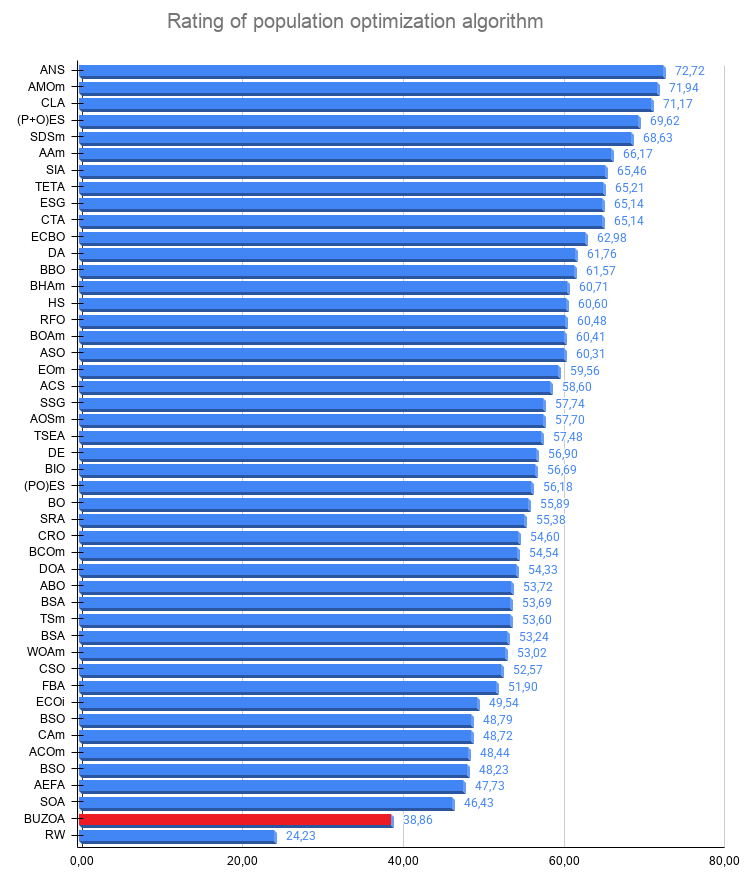
Figure 3. Histogram of the algorithm test results (on a scale from 0 to 100; the higher the score, the better, where 100 is the maximum possible theoretical result); the archive contains a script for calculating the ranking table
Pros and Cons of the Algorithm
Pros:
- It solves simple problems.
Cons:
- Poor performance on high-dimensional problems.
An archive containing the latest versions of the algorithm code is attached to the article. The author of this article does not accept responsibility for the absolute accuracy of the descriptions of the canonical algorithms; many of them have been modified to improve their search capabilities. The conclusions and judgments presented in the articles are based on the results of the experiments conducted.
Files used in this article
| # | Name | Type | Description |
|---|---|---|---|
| 1 | #C_AO.mqh | Include file | Parent class of population-based optimization algorithms |
| 2 | #C_AO_enum.mqh | Include file | Enumeration of population-based optimization algorithms |
| 3 | TestFunctions.mqh | Include file | Test function library |
| 4 | TestStandFunctions.mqh | Include file | Test bench function library |
| 5 | TestStand3D.mqh | Include file | 3D visualization panel for the test bench |
| 6 | Utilities.mqh | Include file | Utility function library |
| 7 | CalculationTestResults.mqh | Include file | Script for calculating results for a comparison table |
| 8 | Test_AO_All.mq5 | Script | Unified test bench for all population-based optimization algorithms |
| 9 | Test_AO_AntiCheat | Script | Cheating test for optimization algorithms |
| 10 | Simple use of population optimization algorithms.mq5 | Script | Simple example of using population-based optimization algorithms without visualization |
| 11 | Test_AO_BUZOA.mq5 | Script | Test bench for BUZOA |
Translated from Russian by MetaQuotes Ltd.
Original article: https://www.mql5.com/ru/articles/21843
Warning: All rights to these materials are reserved by MetaQuotes Ltd. Copying or reprinting of these materials in whole or in part is prohibited.
This article was written by a user of the site and reflects their personal views. MetaQuotes Ltd is not responsible for the accuracy of the information presented, nor for any consequences resulting from the use of the solutions, strategies or recommendations described.

 Automating Chart Patterns in MQL5 (Part 3): The Head and Shoulders and Inverse Head and Shoulders
 Building A Candlestick Trend Constraint Model (Part 11): Revealing Lower-Timeframe Triggers Within Higher-Timeframe Candle Relationships
 Neural Networks in Trading: Iterative Forecast Refinement Models (RAFT)
 Bimodal Market Profile with Delta and Memory in MQL5

- Free trading apps
- Over 8,000 signals for copying
- Economic news for exploring financial markets
You agree to website policy and terms of use