Bull Optimization Algorithm (BOA)

Contents

1. Introduction
2. Implementation of the Algorithm
3. Test Results
4. Conclusions

Introduction

When a trader sets out to optimize the parameters of a trading strategy, they almost always run into the same obstacle: the search space is enormous, the objective function is noisy and has multiple extrema, and there is never as much time and computing power as one would like. The exhaustive search feature in the MetaTrader 5 tester can handle a small number of parameters, but with six to eight variables, the task becomes computationally infeasible. This is where metaheuristic algorithms come into play, but traders then face another problem: which algorithm should they choose?

The most popular candidate is the genetic algorithm (GA), which has been well studied and has been proven effective through decades of practical application. It became the built-in optimizer in MetaTrader 5. Nevertheless, ever since the advent of GA, researchers in the field of metaheuristics have regularly asked: Is it possible to modify the classical framework to obtain an algorithm with a different behavioral profile — one with a different balance between exploration and exploitation, and different mechanisms for information transfer between generations? Such experiments give rise to a family of “genetic operator-based” algorithms, in which the classical GA is just one possible implementation.

In 2015, Turkish researcher Oğuz Fındık published a paper in which he proposed one such experiment. Fındık formulated three observations regarding the behavior of the classical GA that he felt needed to be addressed: the role of the selection operator in population convergence, the nature of classical mutation, and the passive role of the best individual found. Based on these observations, he developed an algorithm with a different architecture: the selection operator is removed from the loop; the best individual becomes an active parent for all the others through crossover; and classical mutation is replaced by multiplicative mutation, proportional to the current value of the gene. The algorithm was named the Bull Optimization Algorithm (BOA).

It is a serious contender, but only algorithms that have proven their effectiveness on our standard benchmark suite deserve a place in our ranking. By the time you finish reading this article, you will have: an understanding of how Fındık’s three architectural decisions come together to form a working algorithm; a breakdown of each decision, complete with a formula and a numerical example; a ready-to-use implementation in MQL5 using the C_AO framework, along with a test script; results from a run on the standard benchmark suite (Hilly, Forest, and Megacity at various search dimensionalities) and on the anti-cheat test suite with five diverse functions; an honest assessment of the problems in which BOA is competitive and those in which its multiplicative mutation works against it.

We will proceed step by step. First, let’s examine exactly which observations about the classical GA Fındık used as the basis for his experiment — without this, the rationale behind his architectural decisions is unclear. Next, let's walk through the BOA structure step by step: initialization, crossover with the leader, multiplicative mutation, chaotic reset, and local search around the best individual. Next — implementation and testing. In conclusion, we'll discuss where BOA excels, where it reaches its limits, and what role it plays in the broader landscape of metaheuristics.

Implementation of the Algorithm

Before delving into the architecture of the new algorithm, it makes sense to consider the three observations that Fındık outlined in his article and work through each one in simple terms.

Observation 1:selection loses its purpose as the population converges. Let’s imagine that a population of 50 individuals has already converged somewhat — they are all in the vicinity of some local maximum, and their fitness values fluctuate, say, in the range from 0.847 to 0.853. Roulette-wheel selection, the most popular selection method in the GA, selects parents with probabilities proportional to their fitness. But for roulette-wheel selection, 0.847 and 0.853 are practically the same. Selection degenerates into random selection, and the algorithm loses “selection pressure” precisely when it is needed most — during the fine-tuning phase.

Observation 2: mutation does not distinguish between “refine” and “throw everything away.” A classic GA mutation for a gene with a range of [-100, 100] works as follows: with probability p_mut, the gene is replaced by a random value from [-100, 100]. If a gene has already reached a value of 0.0023 — close to the optimum — then a mutation will almost certainly push it back somewhere in the range [-87, +43]. That is not “exploring the neighborhood”; it is “throwing away progress.” Therefore, in a GA, the mutation probability has to be kept low (typically 0.01–0.05), but rare mutations are not very effective at escaping local minima.

Observation 3: The best individual is a passive observer. In a classical GA, the best individual is stored separately (elitism), but its genes are not directly passed on to the next generation — it exists in parallel with the evolutionary process. We have an individual whose genes have proven to perform better than those of all the others, but we do not use this information when producing offspring. In this sense, PSO is designed more effectively — in that system, gBest actively pulls all the particles toward itself. The GA, by contrast, prefers to apply crossover to randomly selected parents.

These three observations by the author together formed the basis of BOA. Each is debatable to a different degree — but as a starting point for an experiment, together they form a coherent line of reasoning. The result is an algorithm, which we will now proceed to analyze.

Idea 1: Update all individuals instead of using selection. Fındık removes the selection operator entirely. An individual does not “compete for survival” — it simply lives from iteration to iteration, and at each epoch, its coordinates are recalculated through crossover with the leader and mutation. The best result is stored globally as cB (current Best) and is updated every time an individual produces a fitness value higher than the previous record.

This means that an initially poor individual is not eliminated from the population — it gets a chance to improve through a series of modifications. This is both a strength (we retain diversity) and a risk (if an individual gets stuck in a poor region, it can keep consuming computational resources there).

Idea 2: Always perform crossover with the best individual. Two-point crossover in BOA is designed to be as simple as possible. For each individual i, two integer indices p1 and p2 ∈ [0, D) are generated, where D is the dimensionality of the problem. Let lo = min(p1, p2) and hi = max(p1, p2). Then, for all j ∈ [lo, hi]:

$$x_{ij}\leftarrow {\text{best}}_j$$

$$x_{ij} \leftarrow \text{best}_j$$​That is, the genome segment [lo, hi] is overwritten with a segment from the best individual. This is not a classic segment exchange between two random parents, but rather a targeted “pulling” of a portion of the coordinates toward the leader.

Let D = 6, with individual x = [3.2, -1.5, 0.8, 4.1, 2.0, -0.7] and the best individual best = [1.0, 1.0, 1.0, 1.0, 1.0, 1.0]. The values p1 = 4 and p2 = 1 were generated, meaning lo = 1 and hi = 4. After the crossover:

$$x = [3.2, \mathbf{1.0}, \mathbf{1.0}, \mathbf{1.0}, \mathbf{1.0}, -0.7]$$

The individual now matches the leader in four of its six coordinates.

Idea 3: Multiplicative mutation. This is the most unorthodox part of the algorithm. Mutation formula:

$$v_{ij} = \begin{cases} x_{ij} + \omega \cdot r_1 \cdot x_{ij}, & r_2 \le 0.5 \\ x_{ij} - \omega \cdot r_1 \cdot x_{ij}, & r_2 > 0.5 \end{cases} \quad r_1, r_2 \sim U[0,1]$$

Here, ω is the inertia parameter (mutation scale), and r₁ and r₂ are independent random numbers. The key difference from classical mutation is that the perturbation is proportional to the gene's value itself, rather than to the range of its permissible values.

Let ω = 0.1, x_ij = 5.0, r_1 = 0.6, and r_2 = 0.3. The condition r_2 ≤ 0.5 is satisfied, so:

$$v_{ij} = 5.0 + 0.1 \cdot 0.6 \cdot 5.0 = 5.0 + 0.3 = 5.3$$

Now, let's say that same gene takes on the value x_ij = 0.01 — close to zero. With the same values of ω, r₁, and r₂:

$$v_{ij} = 0.01 + 0.1 \cdot 0.6 \cdot 0.01 = 0.01 + 0.0006 = 0.0106$$

The mutation changed the gene by 0.06% — on a scale consistent with the gene itself. This is a very useful property for functions whose optimum lies near zero: as the coordinate approaches zero, the mutation step also shrinks, and the algorithm converges with high accuracy without the need to manually reduce "ω".

But there is a flip side to this. If the optimum lies, say, at x = 7.0, and the gene happens to pass through zero (for example, following a chaotic mutation), then near zero the mutation step becomes microscopic, and it is nearly impossible to escape from there through ordinary mutation. This is a structural trap in the algorithm, and the only way to escape it is through chaotic mutation — which brings us to the next idea.

Idea 4 (supplementary): chaotic mutation. To give the algorithm a chance to escape from local minima and the “zero trap” of multiplicative mutation, each gene undergoes a random reset with a small probability ChMR (typically 0.001):

$$x_{ij} \leftarrow x_j^{min} + r \cdot (x_j^{max} - x_j^{min}), \quad r \sim U[0,1]$$

This is equivalent to mutation in a classical GA, but it is triggered extremely rarely — on average, one gene per thousand gene updates. This is enough to occasionally move an individual to a random point in the search space, but not enough to undo the progress made.

Idea 5 (supplementary): mutation of the best individual. To enhance local search around the leader, BOA also mutates cB itself using the same formula (11). If the result turns out to be better, cB will be updated. This keeps the leader constantly "jittering" around its current position, which, combined with multiplicative mutation, enables precise convergence in the final epochs.

Linear inertia weight decay. This is not explicitly specified in the article, but the parameters wMax and wMin imply that ω changes over time. We adopt linear inertia weight decay in the spirit of the classical Shi–Eberhart PSO:

$$\omega(t) = \omega_{max} - (\omega_{max} - \omega_{min}) \cdot \frac{t}{T_{max}}$$​

At the start of the optimization, ω = wMax = 0.1 — mutation behaves like a global search. By the end, ω = wMin = 0.0001 — mutation becomes fine local refinement. This scheme provides a classic exploration/exploitation balance, which BOA achieves not by changing the algorithm's structure, but by changing a single parameter.

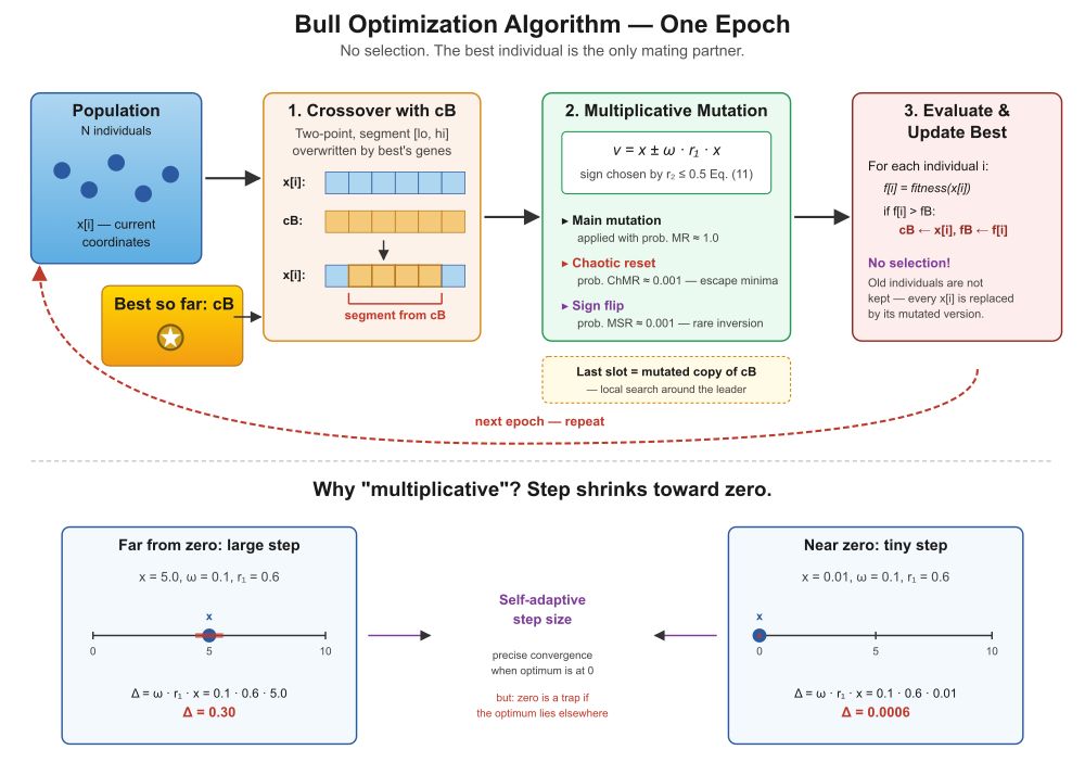
Figure 1. Illustration of how the BOA algorithm works

The illustration consists of two thematic sections:

• Upper section — a single-epoch pipeline: population → crossover with the best individual cB (colored cells show the transfer of a genome segment) → multiplicative mutation with three stages (main / chaotic / sign-flip) → evaluation and update of the best individual, without a selection operator. The last slot, reserved for a mutated copy of cB, is shown separately. The red dashed arrow directs the flow back to the start of the next epoch.
• Lower section — the mechanics of multiplicative mutation: two numerical examples using the same formula, Δ = ω·r₁·x. On the left, x = 5.0 yields Δ = 0.30 (a noticeable step); on the right, x = 0.01 yields Δ = 0.0006 (a microscopic step — the point barely moves). Between the panels is the key takeaway: a self-adjusting step size that enables precise convergence to zero but turns zero itself into a trap when the optimum is shifted away from zero.

Now let's write the pseudocode for the algorithm.

INITIALIZATION:
    Set parameters: popSize, CR, MR, MSR, ChMR, ω_max, ω_min
    epochs   ← number of optimization epochs
    epochNow ← 0
    ω        ← ω_max

    For each individual i = 1 … popSize:
        For each coordinate c = 1 … D:
            x[i][c] ← random(rangeMin[c], rangeMax[c])    // Eq. (10)

MAIN LOOP (repeat till completion):

    // ──────────── EVALUATION ────────────
    Calculate fitness f[i] for all population individuals

    // ──────────── UPDATE BESTS ────────────
    For each individual i:
        If f[i] > fB[i] (personal record):
            fB[i] ← f[i];  cB_pers[i] ← x[i]
        If f[i] > fB (global record):
            fB ← f[i];     cB ← x[i]

    // ──────────── INERTIA WEIGHT DECAY ────────────
    epochNow ← epochNow + 1
    ω ← ω_max − (ω_max − ω_min) · (epochNow / epochs)

    // ──────────── POPULATION UPDATE ────────────
    // The last slot is reserved for a mutated copy of the leader → process slots 1 through popSize-1
    For each individual i = 1 … popSize − 1:

        // ─── STEP 1. Crossover with the best individual cB ───
        If random(0,1) ≤ CR:
            p1 ← randInt(0, D);   p2 ← randInt(0, D)
            lo ← min(p1, p2);     hi ← max(p1, p2)
            For c = lo … hi:
                x[i][c] ← cB[c]                            // overwrite the region with the leader's genes

        // ─── STEP 2. Multiplicative mutation (Eq. 11) ───
        For each coordinate c = 1 … D:
            v ← x[i][c]

            If random(0,1) ≤ MR:
                r1 ← random(0,1);   r2 ← random(0,1)
                If r2 ≤ 0.5:
                    v ← v + ω · r1 · v                     // Eq. (11), the "+" sign
                Otherwise:
                    v ← v − ω · r1 · v                     // Eq. (11), the "−" sign

            // ─── STEP 3. Chaotic mutation (escape from local minima) ───
            If random(0,1) ≤ ChMR:
                v ← random(rangeMin[c], rangeMax[c])

            // ─── STEP 4. Sign-flip mutation (rare inversion) ───
            If random(0,1) ≤ MSR:
                v ← −v

            x[i][c] ← clamp(v, rangeMin[c], rangeMax[c])

    // ─── STEP 5. Local search around the leader ───
    // Last population slot = mutated copy of cB
    For each coordinate c = 1 … D:
        v ← cB[c]

        If random(0,1) ≤ MR:
            r1 ← random(0,1);   r2 ← random(0,1)
            If r2 ≤ 0.5:  v ← v + ω · r1 · v
            Otherwise:          v ← v − ω · r1 · v

        If random(0,1) ≤ ChMR:
            v ← random(rangeMin[c], rangeMax[c])

        If random(0,1) ≤ MSR:
            v ← −v

        x[popSize][c] ← clamp(v, rangeMin[c], rangeMax[c])

RETURN: cB, fB

Let's start implementing the algorithm.

The C_AO_BOA_Bull class. This class inherits from the base class C_AO — the standard interface of the population-based algorithms framework. This gives it the entire infrastructure “for free”: an array of agents a[] with coordinates c[]/cP[]/cB[]/cW[] and fitness values f/fP/fB/fW, global variables cB and fB for the best individual, an array of parameters params[], utilities “u” (random number generators, discretization, boundary checks), as well as the standard life cycle Init() → Moving() → Revision(). The algorithm implementer only needs to define three virtual methods, as done here.

Algorithm parameters (declared as public fields for transparency):

• CR — crossover rate, the probability that a two-point crossover will be applied to an individual in each epoch. When CR = 1.0 (the default value from the article), the crossover is always applied.
• MR — mutation rate, the probability of applying the main multiplicative mutation to each coordinate. The default value of 1.0 means that each gene is processed using Equation (11) at every epoch.
• MSR — mutation sign rate, the probability of a rare coordinate sign inversion. Fındık mentions this parameter but does not define it with a formula; the interpretation adopted here is x ← -x with a low probability (≈0.001).
• ChMR — chaotic mutation rate, the probability that a coordinate will undergo a random reset to a random point within the valid range. The only mechanism capable of pulling an agent out of the local minima into which it is driven by multiplicative mutation.
• wMax, wMin — the upper and lower bounds of the inertia weight ω, which decreases linearly from wMax to wMin as optimization progresses. It controls the balance between exploration and exploitation: mutations are large at the beginning and microscopic by the end.

Private fields (internal fields for controlling the inertia weight):

• epochs — the total number of epochs passed during initialization; required for calculating the linear decay of the inertia weight ω.
• epochNow — a counter for the current epoch, which is incremented in Revision.
• wCur — the current inertia weight, recalculated at each epoch.
• Clamp is a private utility that clamps the value to the bounds [lo, hi]. It is used after a mutation because a multiplicative mutation can cause a coordinate to fall outside the valid range.

The C_AO_BOA_Bull() constructor populates three internal fields of the base class (ao_name, ao_desc, ao_link), which are used to identify the algorithm in logs and the interface. It then sets the default parameter values and registers them in the params[] array. Each parameter is registered using two fields — name for display and val for its value — so that an external script can both read parameters by name and override their values through the standard interface.

The SetParams() method. This reverses the constructor's operation by transferring values from the params[] array back into the class's named fields. This is called after an external script has updated `params[i].val` with its input values. Without this step, the class would use the default values, ignoring the user's configuration.

//+------------------------------------------------------------------+
class C_AO_BOA_Bull : public C_AO
 {
public:
                    ~C_AO_BOA_Bull() {}
                     C_AO_BOA_Bull()
   {
    ao_name = "BOA";
    ao_desc = "Bull Optimization Algorithm";
    ao_link = "https://www.mql5.com/en/articles/22390";

    popSize = 50;
    CR      = 1.0;
    MR      = 1.0;
    MSR     = 0.001;
    ChMR    = 0.001;
    wMax    = 0.1;
    wMin    = 0.0001;

    ArrayResize(params, 7);
    params [0].name = "popSize"; params [0].val = popSize;
    params [1].name = "CR";      params [1].val = CR;
    params [2].name = "MR";      params [2].val = MR;
    params [3].name = "MSR";     params [3].val = MSR;
    params [4].name = "ChMR";    params [4].val = ChMR;
    params [5].name = "wMax";    params [5].val = wMax;
    params [6].name = "wMin";    params [6].val = wMin;
   }

  void               SetParams()
   {
    popSize = (int)params [0].val;
    CR      = params      [1].val;
    MR      = params      [2].val;
    MSR     = params      [3].val;
    ChMR    = params      [4].val;
    wMax    = params      [5].val;
    wMin    = params      [6].val;
   }

  bool               Init(const double &rangeMinP  [],
                          const double &rangeMaxP  [],
                          const double &rangeStepP [],
                          const int     epochsP = 0);

  void               Moving();
  void               Revision();

  //------------------------------------------------------------------
  double             CR;    // crossover rate                       [0..1]
  double             MR;    // mutation rate                        [0..1]
  double             MSR;   // mutation sign rate (rare sign inversion) [≈0.001]
  double             ChMR;  // chaotic mutation rate                [≈0.001]
  double             wMax;  // ω_max — mutation scale at the start     [≈0.1]
  double             wMin;  // ω_min — mutation scale at the end [≈0.0001]

private: //----------------------------------------------------------
  int                epochs;   // total number of epochs (for linear decay of ω)
  int                epochNow; // current epoch number
  double             wCur;     // current inertia weight

  double             Clamp(double v, double lo, double hi)
   {
    return v < lo ? lo : v > hi ? hi : v;
   }
 };
//+------------------------------------------------------------------+

The Init method. Preparation for running the optimization.

The first line — StandardInit() — calls a procedure inherited from C_AO that initializes the population size and the array of agents, copies the search ranges into internal fields, and resets the best and worst fitness values found to zero. If standard initialization fails (for example, if the dimensionality of the problem is 0 or the array sizes are inconsistent), Init() returns false and nothing else happens.

Next, the number of epochs is saved (with protection against division by zero via `epochsP > 0 ? epochsP : 1`), the current epoch counter is reset to zero, and `wCur` is set to the initial value `wMax` — the starting point for the inertia weight decay.

The main substantive part is a nested loop that implements equation (10) from the article: each coordinate of each agent is initialized with a random value from the valid range. The values are stored in cP[] (previous coordinates) because Moving() expects the “previous position” and uses it to calculate the “current position,” with quantization to the grid spacing.

//+------------------------------------------------------------------+
bool C_AO_BOA_Bull::Init(const double &rangeMinP  [],
                         const double &rangeMaxP  [],
                         const double &rangeStepP [],
                         const int     epochsP = 0)
 {
  if(!StandardInit(rangeMinP, rangeMaxP, rangeStepP))
    return false;

  epochs   = epochsP > 0 ? epochsP : 1;
  epochNow = 0;
  wCur     = wMax;

//--- Eq. (10): Initial population in [rangeMin, rangeMax]
  for(int i = 0; i < popSize; i++)
    for(int c = 0; c < coords; c++)
      a [i].cP [c] = u.RNDfromCI(rangeMin [c], rangeMax [c]);

  return true;
 }
//+------------------------------------------------------------------+

The Moving() method. It is executed first in each epoch of the optimizer, before the fitness is calculated. Its task is to prepare the coordinates for evaluation.

In BOA, the method is trivial: it simply copies "cP" to "c", but does so using the u.SeInDiSp() utility, which does two things. First, it clamps the value to the [rangeMin, rangeMax] bounds (to prevent the search from going out of bounds). Second, it quantizes the value to the grid spacing `rangeStep` — if `rangeStep[c] = 0.5`, the coordinate is rounded to the nearest multiple of 0.5. For most problems, `rangeStep = 0` and discretization is disabled, but for discrete problems (such as Megacity and similar ones), this step is critical.

There is no position-update logic here — all the algorithm's work is concentrated in Revision(). This is a distinctive feature of BOA: positions are recalculated after evaluation, not before. In a typical epoch, fitness evaluation comes first, followed by the position update — in the next epoch, the new positions are passed to Moving() via cP.

//+------------------------------------------------------------------+
void C_AO_BOA_Bull::Moving()
 {
  for(int i = 0; i < popSize; i++)
    for(int c = 0; c < coords; c++)
      a [i].c [c] = u.SeInDiSp(a [i].cP [c], rangeMin [c], rangeMax [c], rangeStep [c]);
 }
//+------------------------------------------------------------------+

The Revision() method is the heart of the algorithm. It is called after the fitness function has evaluated all agents. It consists of four blocks that sequentially update the population.

Block 1: Updating personal and global bests. A standard loop: for each agent, if its current fitness f is better than its personal best fB, update the personal best and copy the coordinates to a[i].cB. We also compare each agent's current fitness with the class-wide global fB; if an agent improves on it, we update the global fB and cB. The global cB is the “bull”: the leader that will serve as the crossover partner for the entire population.

Block 2: Linear Inertia Weight Decay. The epoch counter is incremented, and wCur is recalculated using a linear interpolation formula: the more epochs have elapsed, the smaller ω becomes. The safeguard check `if(wCur < wMin)` is triggered when `epochNow` exceeds the specified `epochs` (which can happen with a variable run length) — ω is clamped to its minimum rather than becoming negative, which would break the mutation mechanism.

Block 3: Main Loop — Population Update Without Selection. This is where the key concept of BOA comes into play. The loop runs from 0 to popSize - 2 (that is, it processes all agents except the last one — that slot is reserved for block 4).

Within the loop, each agent goes through two phases:

• Phase 3.1 — Two-point crossover with cB. With probability CR, the following procedure is initiated: two integer indices in the range [0, coords) are generated using (int)u.RNDfromCI(0.0, coords). The safety checks `if(p1 >= coords) p1 = coords - 1` are necessary in case the random number generator returns a value exactly equal to `coords` due to rounding. Next, the interval [lo, hi] is defined from the smaller index to the larger index, and within this interval, the agent's coordinates are overwritten with those of the leader. This is not a symmetric exchange of segments as in a classical GA — it is a one-way “pull” of part of the genome toward the best individual.
• Phase 3.2 — Coordinate mutation. Three independent events are checked sequentially for each coordinate.

First, the main multiplicative mutation according to formula (11). With probability MR (usually 1.0), r1 and r2 are drawn from U[0,1]. If r2 ≤ 0.5, the coordinate increases by ω·r1·v; otherwise, it decreases by the same amount. The step size is proportional to the coordinate value itself — this is what is meant by “multiplicativity”: near zero, the step size is tiny; far from zero, it is significant.

Second, a chaotic mutation with a probability of ChMR (usually 0.001). The coordinate is reset to a random point within the valid range. This is the only mechanism for global search after the main mutation has driven the coordinates to small values.

Third, a sign-flip mutation with a probability of MSR (usually 0.001). The coordinate changes sign: v ← -v. It is useful for symmetric functions, where the optimum may lie at the mirror point across zero.

After all three mutations, the result is clamped to the bounds using Clamp() and written back to the agent's cP[] — in the next epoch, Moving() will retrieve this value and pass it to the fitness function.

Block 4: Local search around the leader. The last slot in the population (popSize - 1) is filled with a mutated copy of cB at each epoch. The mutation logic is the same as in Block 3.2 — three stages with the same probabilities, but the starting point is the leader itself rather than the current agent's coordinates.

This trick solves an important problem: in BOA, the leader does not move on its own; it can only be updated when another agent happens to stumble upon a better spot. A mutated leader slot gives the leader a chance to improve on its own — if the mutation results in a higher fitness, Block 1 will update cB to that value in the next epoch. This can be viewed as a built-in “local search” within the population-based algorithm, without the overhead of a separate mechanism. The cost of this solution is that one agent out of 50 is not used as an independent search unit, but serves as a “mirror” for the leader.

//+------------------------------------------------------------------+
void C_AO_BOA_Bull::Revision()
 {
//--- 1. Update personal and global bests ------------------
  for(int i = 0; i < popSize; i++)
   {
    if(a [i].f > a [i].fB)
     {
      a [i].fB = a [i].f;
      ArrayCopy(a [i].cB, a [i].c, 0, 0, coords);
     }
    if(a [i].f > fB)
     {
      fB = a [i].f;
      ArrayCopy(cB, a [i].c, 0, 0, coords);
     }
   }

//--- 2. Linear inertia weight decay: ω_max → ω_min --------------------
  epochNow++;
  wCur = wMax - (wMax - wMin) * ((double)epochNow / (double)epochs);
  if(wCur < wMin)
    wCur = wMin;

//--- 3. Population update (no selection—an individual is always
//       replaced by the result of crossover + mutation) ---------------
//
// WARNING: One slot (the last one) is reserved for a mutated
// version of gBest—to enhance local search around the leader.
//
  int N = popSize - 1;

  for(int i = 0; i < N; i++)
   {
    //--- 3.1 Two-point crossover with the best individual ---------------
    if(u.RNDfromCI(0.0, 1.0) <= CR)
     {
      int p1 = (int)u.RNDfromCI(0.0, (double)coords);
      int p2 = (int)u.RNDfromCI(0.0, (double)coords);
      if(p1 >= coords)
        p1 = coords - 1;
      if(p2 >= coords)
        p2 = coords - 1;
      int lo = p1 < p2 ? p1 : p2;
      int hi = p1 < p2 ? p2 : p1;
      for(int c = lo; c <= hi; c++)
        a [i].cP [c] = cB [c];
     }

    //--- 3.2 Mutation according to Eq. (11) + chaotic mutation + sign-flip mutation ---------
    for(int c = 0; c < coords; c++)
     {
      double v = a [i].cP [c];

      // Primary mutation: v = v ± ω·r1·v
      if(u.RNDfromCI(0.0, 1.0) <= MR)
       {
        double r1 = u.RNDfromCI(0.0, 1.0);
        double r2 = u.RNDfromCI(0.0, 1.0);
        if(r2 <= 0.5)
          v = v + wCur * r1 * v;
        else
          v = v - wCur * r1 * v;
       }

      // Chaotic mutation: random reset within [min, max]
      if(u.RNDfromCI(0.0, 1.0) <= ChMR)
        v = u.RNDfromCI(rangeMin [c], rangeMax [c]);

      // Sign-flip mutation: a rare gene sign inversion
      if(u.RNDfromCI(0.0, 1.0) <= MSR)
        v = -v;

      a [i].cP [c] = Clamp(v, rangeMin [c], rangeMax [c]);
     }
   }

//--- 4. Local search around the leader ---------------------------
// The last slot is filled with a mutated copy of cB.
// If it turns out to be better, fB will be updated in the next iteration.
  for(int c = 0; c < coords; c++)
   {
    double v = cB [c];

    if(u.RNDfromCI(0.0, 1.0) <= MR)
     {
      double r1 = u.RNDfromCI(0.0, 1.0);
      double r2 = u.RNDfromCI(0.0, 1.0);
      if(r2 <= 0.5)
        v = v + wCur * r1 * v;
      else
        v = v - wCur * r1 * v;
     }

    if(u.RNDfromCI(0.0, 1.0) <= ChMR)
      v = u.RNDfromCI(rangeMin [c], rangeMax [c]);

    if(u.RNDfromCI(0.0, 1.0) <= MSR)
      v = -v;

    a [popSize - 1].cP [c] = Clamp(v, rangeMin [c], rangeMax [c]);
   }
 }
//+------------------------------------------------------------------+

Test Results

The final score of 46.39% on the full benchmark suite is a fraction of a percentage point below the threshold for making the top 45. The algorithm does not appear in the ranking table. Dimensionality proved to be the deciding factor: on 5-dimensional problems, BOA performs in the top third of the rankings; on 25-dimensional problems, it performs in the middle; and on 500-dimensional problems, it fails. The reason is structural: at a dimensionality of 500, multiplicative mutation v = x ± ω·r·x produces such a small step along each coordinate that chaotic mutation, with a probability of 0.001, becomes the only effective exploration mechanism — and 0.5 events per epoch is simply not enough for a 500-dimensional space.

BOA|Bull Optimization Algorithm|50.0|1.0|0.1|0.01|0.001|0.1|0.0001|
=============================
5 Hilly's; Func runs: 10000; result: 0.7128139073590452
25 Hilly's; Func runs: 10000; result: 0.5190082455068694
500 Hilly's; Func runs: 10000; result: 0.28947759543651924
=============================
5 Forest's; Func runs: 10000; result: 0.9696150570558139
25 Forest's; Func runs: 10000; result: 0.38037078784762096
500 Forest's; Func runs: 10000; result: 0.06579884061143552
=============================
5 Megacity's; Func runs: 10000; result: 0.7253333333333333
25 Megacity's; Func runs: 10000; result: 0.376
500 Megacity's; Func runs: 10000; result: 0.1366933333333343
=============================
All score: 4.17511 (46.39%)

An anti-bias test on five different functions with widely separated optima confirmed that BOA's low-dimensional results on the standard benchmark suite are not an artifact — the algorithm genuinely finds compromise solutions across heterogeneous landscapes. Forest 10D = 0.97 does not “cheat” by using diagonal contraction, as was the case with HHO; the crossover with the leader pulls the population toward the true optimum, rather than toward a fortunate coincidence between the nature of the test function and the algorithm’s architecture.

BOA|Bull Optimization Algorithm|50.0|1.0|0.1|0.01|0.001|0.1|0.0001|
=============================
Composite test: Hilly + Forest + Megacity + Peaks + Skin
Coordinates: 10; Epochs: 200; Repeats: 10
=============================
Run 1/10: 0.8534132121249
Run 2/10: 0.7319045719778601
Run 3/10: 0.9835678308131334
Run 4/10: 0.9799860818205021
Run 5/10: 0.9799860818205021
Run 6/10: 0.7128042825713253
Run 7/10: 0.9456553720712788
Run 8/10: 0.9456553720712788
Run 9/10: 0.8871885236634757
Run 10/10: 0.6966858914401158
=============================
Average result: 0.8716847220 (87.17%)
=============================

Visualization of the algorithm in action on test functions and on functions supplied with the program.

BOA on the Hilly test function

BOA on the Forest test function

BOA on the Megacity test function

BOA on the Ackley function

BOA on the Peaks function

The BOA algorithm is presented in the ranking table for informational purposes only.

AO	Description	Hilly			Hilly Final	Forest			Forest Final	Megacity (discrete)			Megacity Final	Final Result	% of MAX
		10 p (5 F)	50 p (25 F)	1,000 p (500 F)		10 p (5 F)	50 p (25 F)	1,000 p (500 F)		10 p (5 F)	50 p (25 F)	1,000 p (500 F)
ANS	across neighbourhood search	1.00000	0.88228	0.40138	2.28366	1.00000	0.95281	0.28092	2.23373	0.94667	0.85733	0.22389	2.02789	6.545	72.72
AMOm	animal migration optimization M	0.91624	0.83603	0.46790	2.22017	0.98482	0.92010	0.36391	2.26883	0.91733	0.81707	0.25177	1.98617	6.475	71.94
CLA	code lock algorithm (joo)	0.95139	0.86199	0.37879	2.19217	0.99349	0.93500	0.26497	2.19346	0.93600	0.84267	0.24060	2.01927	6.405	71.17
(P+O)ES	(P+O) evolution strategies	0.86571	0.89539	0.39740	2.15850	0.97761	0.89820	0.26878	2.14459	0.92133	0.80240	0.23952	1.96325	6.266	69.62
SDSm	stochastic diffusion search M	0.95195	0.84944	0.36249	2.16388	0.98061	0.88457	0.22112	2.08630	0.92267	0.79013	0.21380	1.92660	6.177	68.63
AAm	archery algorithm M	0.84685	0.73320	0.42590	2.00595	0.96709	0.77837	0.27789	2.02335	0.86133	0.77707	0.28712	1.92552	5.955	66.17
SIA	simulated isotropic annealing (joo)	0.93543	0.86504	0.38483	2.18530	0.94069	0.80609	0.23835	1.98513	0.86400	0.66160	0.19536	1.72096	5.891	65.46
TETA	time evolution travel algorithm (joo)	0.91452	0.86369	0.25579	2.03400	0.99654	0.91291	0.14394	2.05339	0.85467	0.82213	0.10443	1.78123	5.869	65.21
ESG	evolution of social groups (joo)	0.98111	0.79857	0.31167	2.09135	0.98954	0.82270	0.15032	1.96256	0.92133	0.73440	0.15315	1.80888	5.863	65.14
CTA	comet tail algorithm (joo)	0.92435	0.86786	0.27838	2.07059	0.99039	0.84571	0.19448	2.03058	0.95467	0.69680	0.11008	1.76155	5.863	65.14
ECBO	enhanced colliding bodies optimization	0.94024	0.72363	0.32356	1.98743	0.99477	0.80291	0.13056	1.92824	0.87600	0.70160	0.17433	1.75193	5.668	62.98
DA	dialectical algorithm	0.93117	0.75400	0.26205	1.94722	0.98925	0.81375	0.08662	1.88962	0.92667	0.68107	0.11315	1.72089	5.558	61.76
BBO	biogeography-based optimization	0.95876	0.70609	0.35752	2.02237	0.92981	0.70660	0.16970	1.80611	0.87467	0.63013	0.20813	1.71293	5.541	61.57
BHAm	black hole algorithm M	0.79558	0.76207	0.34682	1.90447	0.99836	0.75798	0.13826	1.89460	0.85067	0.64427	0.17020	1.66514	5.464	60.71
HS	harmony search	0.91420	0.69049	0.29924	1.90393	0.97627	0.73373	0.14193	1.85193	0.91733	0.62720	0.15364	1.69817	5.454	60.60
RFO	royal flush optimization (joo)	0.80989	0.74481	0.34546	1.90016	0.95251	0.77926	0.15185	1.88362	0.80400	0.66427	0.19071	1.65898	5.443	60.48
BOAm	billiards optimization algorithm M	0.76177	0.72421	0.25275	1.73873	0.90890	0.81960	0.28853	2.01703	0.83733	0.74613	0.09763	1.68109	5.437	60.41
ASO	anarchy society optimization	0.73070	0.73713	0.31195	1.77978	0.99732	0.87700	0.17619	2.05051	0.72000	0.68773	0.18988	1.59761	5.428	60.31
EOm	extremal Optimization_M	0.76527	0.75205	0.31908	1.83640	0.99999	0.76426	0.12437	1.88862	0.84133	0.64133	0.15247	1.63513	5.360	59.56
ACS	artificial cooperative search	0.75545	0.77162	0.31653	1.84360	1.00000	0.80488	0.10705	1.91193	0.76933	0.60800	0.14157	1.51890	5.274	58.60
SSG	saplings sowing and growing	0.75436	0.63206	0.35935	1.74577	0.91907	0.69694	0.19755	1.81356	0.81867	0.60533	0.21347	1.63747	5.197	57.74
AOSm	atomic orbital search M	0.76184	0.68435	0.31344	1.75963	0.90015	0.80044	0.11501	1.81560	0.82800	0.63280	0.15696	1.61776	5.193	57.70
TSEA	turtle shell evolution algorithm (joo)	0.95809	0.64852	0.29571	1.90232	0.99522	0.58104	0.10542	1.68168	0.92133	0.52160	0.14567	1.58860	5.173	57.48
DE	differential evolution	0.96398	0.62346	0.26089	1.84833	0.98482	0.77018	0.11459	1.86959	0.93067	0.36213	0.11000	1.40280	5.121	56.90
BIO	blood inheritance optimization (joo)	0.72580	0.66522	0.31228	1.70330	0.99995	0.68125	0.11540	1.79660	0.85467	0.59333	0.15364	1.60164	5.102	56.69
(PO)ES	(PO) evolution strategies	0.73972	0.58190	0.38896	1.71058	0.91199	0.59975	0.21262	1.72436	0.82400	0.56240	0.23432	1.62072	5.056	56.18
BO	bonobo optimizer	0.75555	0.64366	0.32657	1.72578	0.94332	0.70442	0.13999	1.78773	0.73467	0.61440	0.16728	1.51635	5.030	55.89
SRA	successful restaurateur algorithm (joo)	0.89010	0.63359	0.29115	1.81484	0.96634	0.55285	0.08914	1.60833	0.89333	0.52800	0.13911	1.56044	4.984	55.38
CRO	chemical reaction optimisation	0.91281	0.65681	0.29866	1.86828	0.90513	0.56020	0.10939	1.57472	0.82800	0.50133	0.14149	1.47082	4.914	54.60
BCOm	bacterial chemotaxis optimization M	0.82589	0.61733	0.31584	1.75906	0.95296	0.63718	0.11984	1.70998	0.76533	0.51653	0.15800	1.43986	4.909	54.54
DOA	dream optimization algorithm	0.78522	0.78121	0.36036	1.92679	0.61584	0.42117	0.12254	1.15955	0.86667	0.72587	0.21127	1.80381	4.890	54.33
ABO	african buffalo optimization	0.92295	0.62528	0.29885	1.84708	0.92992	0.57468	0.09372	1.59832	0.73333	0.51333	0.14324	1.38990	4.835	53.72
BSA	bird swarm algorithm	0.94432	0.67941	0.26401	1.88774	0.91649	0.65619	0.12054	1.69322	0.80933	0.33547	0.10652	1.25132	4.832	53.69
TSm	tabu search M	0.87806	0.61040	0.28993	1.77839	0.98116	0.52165	0.08544	1.58825	0.82667	0.49547	0.13552	1.45766	4.824	53.60
BSA	backtracking search algorithm	0.87128	0.53190	0.28675	1.68993	0.92408	0.51602	0.09153	1.53163	0.96000	0.47253	0.13760	1.57013	4.792	53.24
WOAm	whale optimization algorithm M	0.93893	0.59477	0.26695	1.80065	0.98036	0.53873	0.07112	1.59021	0.78667	0.47600	0.11892	1.38159	4.772	53.02
CSO	competitive swarm optimizer	0.85151	0.60786	0.29896	1.75833	0.84085	0.58491	0.11974	1.54550	0.80000	0.48560	0.14184	1.42744	4.731	52.57
FBA	fractal-based algorithm	0.69419	0.64267	0.28955	1.62641	0.99812	0.54905	0.08705	1.63422	0.76133	0.51253	0.13689	1.41075	4.671	51.90
ECOi	eco-inspired evolutionary algorithm	0.78817	0.54402	0.29360	1.62579	0.88996	0.46592	0.09747	1.45335	0.78533	0.45173	0.14295	1.38001	4.459	49.54
BSO	brain storm optimization	0.92207	0.57625	0.29732	1.79564	0.80764	0.42508	0.09448	1.32720	0.77200	0.36533	0.13065	1.26798	4.391	48.79
CAm	camel algorithm M	0.71534	0.56917	0.35985	1.64436	0.84094	0.47174	0.10850	1.42118	0.70400	0.41947	0.19563	1.31910	4.385	48.72
ACOm	ant colony optimization_M	0.71885	0.48410	0.30990	1.51285	0.75792	0.48639	0.11871	1.36302	0.83600	0.48667	0.16148	1.48415	4.360	48.44
BSO	brain storm optimization	0.91331	0.55813	0.29705	1.76849	0.85329	0.44038	0.09447	1.38814	0.72267	0.32880	0.13325	1.18472	4.341	48.23
AEFA	artificial electric field algorithm	0.88798	0.65769	0.25276	1.79843	0.95550	0.63602	0.03946	1.63098	0.60800	0.16000	0.09845	0.86645	4.296	47.73
SOA	simple optimization algorithm	0.91664	0.47040	0.27095	1.65799	0.88264	0.31546	0.06044	1.25854	0.82933	0.31733	0.11579	1.26245	4.179	46.43
BOA_Bull	bull_optimization_algorithm	0.71281	0.51900	0.28947	1.52128	0.96961	0.38037	0.06579	1.41577	0.72533	0.37600	0.13669	1.23802	4.175	46.39
RW	random walk	0.49970	0.32333	0.25791	1.08094	0.30754	0.11470	0.04400	0.46624	0.36133	0.17013	0.10244	0.63390	2.181	24.23

Conclusions

In 2015, Oğuz Fındık formulated three criticisms of the classical GA — selection that degenerates as convergence occurs, destructive mutation far from the range, and the passive role of the elite individual — and proposed three targeted solutions: eliminate selection entirely, make the best individual a mandatory mating partner for all others, and replace additive mutation with multiplicative mutation.

At the beginning of this article, we outlined the problem faced by a trader who hits a wall when optimizing strategy parameters: the space is vast, and the objective function has multiple extrema. After going through this material, the trader will have three tools at their disposal.

First, the implementation of BOA in the C_AO format, ready to be integrated alongside any other algorithm in the framework. For optimization problems with 5–25 parameters (which is typically the number found in an average trading strategy — indicator periods, SL/TP levels, volatility filters, and weights in composite signals), BOA delivers results comparable to those of algorithms in the rankings. It's not the best tool in the toolbox, but it's a useful tool with a sound underlying mechanism, and it has a place in a portfolio of optimizers — especially when fast convergence and precise refinement around an identified extremum are needed.

Second, understanding which tasks BOA does not address. If portfolio optimization involves 100 or more parameters (such as weights in a large system), BOA is not a suitable choice: its multiplicative mutation is inherently unable to scale to such high dimensionality. In this case, it is best to choose algorithms near the top of the rankings that have demonstrated robustness at high dimensionality.

Third, understanding the very concept of a multiplicative step. This is a clever engineering solution: a perturbation step automatically scaled to the magnitude of the variable itself. The idea is not specific to BOA and can be adapted to other algorithms — such as hybrids with PSO and DE, or custom solutions for specific trading tasks. The seven BOA configuration parameters (CR, MR, MSR, ChMR, wMax, wMin, popSize) provide ample scope for experimentation.

The algorithm is available to the public, and I invite anyone interested to experiment with the parameters. In today's rankings, BOA is in the "did not make the cut, but came close" category. That's a fair result. But that does not mean the work is a failure: the three ideas presented in the author's article are worth exploring on their own, and their implementation demonstrates exactly how they work together.

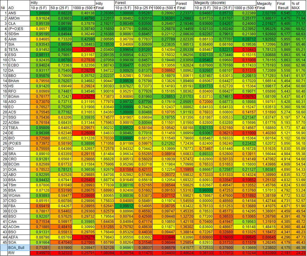
Figure 2. Color coding of algorithms by their results on the respective tests

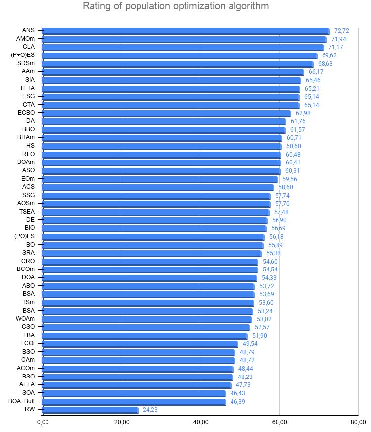
Figure 3. A histogram of the algorithm test results (on a scale from 0 to 100; the higher the score, the better, where 100 is the maximum possible theoretical result); the archive contains a script for calculating the ranking table

Pros and Cons of the Algorithm

Pros:

1. Solves problems of up to medium dimensionality.

Cons:

1. A large number of external parameters.
2. A tendency to get stuck on certain types of problems.

An archive containing the latest versions of the algorithm source code is attached to the article. The author of this article does not guarantee complete accuracy in the descriptions of canonical algorithms; many of these algorithms have been modified to improve their search capabilities. The conclusions and judgments presented in the articles are based on the results of the experiments conducted.

• GitHub: https://github.com/JQSakaJoo/Population-optimization-algorithms-MQL5

Software used in this article

#	Name	Type	Description
1	#C_AO.mqh	Include file	Parent class for population-based optimization algorithms
2	#C_AO_enum.mqh	Include file	Enumeration of population-based optimization algorithms
3	TestFunctions.mqh	Include file	Test function library
4	TestStandFunctions.mqh	Include file	Benchmark suite function library
5	TestStand3D.mqh	Include file	3D visualization panel for the benchmark suite
6	Utilities.mqh	Include file	Utility functions library
7	CalculationTestResults.mqh	Include file	Script for calculating results for the comparison table
8	Test_AO_All.mq5	Script	Unified benchmark suite for all population-based optimization algorithms
9	Test_AO_AntiCheat	Script	Test for cheating in optimization algorithms
10	Simple use of population optimization algorithms.mq5	Script	Simple example of using population-based optimization algorithms without visualization
11	Test_AO_BOA.mq5	Script	Benchmark suite for BOA