

Network Momentum for MetaTrader5: Trading the Lead-Lag Graph Between Markets
 1 360
1 360
 2
2

Introduction
Most trend-following systems treat each market as an island, asking one question in isolation: is the price trending up or down right now? The moving-average crossover, the MACD and the breakout channel — all of them read one series and act on that series alone. This works, and it has worked for decades, but it quietly throws away a large piece of information: markets do not move independently. A move in crude oil bleeds into the currencies of oil exporters. A turn in an equity index leads the risk-sensitive currencies that track it. A shift in metals shows up later in the commodity dollars. When one market consistently moves before another, the leader's trend today is a clue about where the lagger goes tomorrow. This is momentum spillover, and it is invisible to any indicator that looks at one chart at a time.
In this article we build an Expert Advisor that reads a basket of markets rather than one chart at a time. It infers which of them tend to lead which, assembles those lead-lag relationships into a weighted network, and lets each market's momentum flow along the edges to its neighbours. The result is a single number per symbol, a network momentum signal, whose sign decides whether we go long, short, or flat. The method comes from a 2025 research paper, and the implementation is done entirely in MQL5, with no Python, no external solver, and no pre-computed files: the EA gathers its own data, learns the graph on the fly, and trades the signal it computes.
The strategy is a faithful implementation of the paper's Derivative Dynamic Time Warping pipeline, adapted from the paper's commodity-futures universe to a basket of foreign-exchange pairs and cross-asset instruments that a retail MetaTrader 5 account actually carries. We will walk through the theory, then build the engine module by module in pure MQL5, wire it into a live EA, and finish by running it on the Strategy Tester to confirm the whole machine works end to end and trades coherently.
We will cover:
- The Idea: Momentum That Spills Between Markets
- From Lead-Lag to a Network: The Theory
- Architecture of the Implementation
- Volatility Scaling and the Oscillators
- Detecting the Leaders: DDTW
- Learning the Graph
- The Engine: Ensemble, Propagation and Signal
- Bringing It Live: The EA
- Testing on the Strategy Tester
- Conclusion
The Idea: Momentum That Spills Between Markets
Trend-following rests on a simple premise: price direction tends to persist. Assets whose prices have been rising tend to keep rising, and those that have been falling tend to keep falling, so a trader can profit by buying recent winners and selling recent losers in the expectation that the trend continues. This persistence has been studied and validated extensively, and it produces the characteristic payoff of a good trend-follower: many small losses compensated by fewer but much larger gains, which shows up statistically as positive skew in the return distribution.
The persistence is not confined to a single market. A large body of research documents that returns spill across markets: high equity returns in one year can predict high corporate-bond returns the next, currency news leads bonds in emerging markets, crude-oil volatility leads global equities. This cross-market persistence is called the lead-lag effect: one market's trending behaviour arrives, with a delay, in another. The delay comes from real frictions, the slow diffusion of information, delayed reactions, and asynchronous response timings across participants and asset classes.
The paper this article implements is Follow the Leader: Enhancing Systematic Trend-Following Using Network Momentum by Linze Li and William Ferreira (2025). Its central move is to measure these lead-lag relationships across a whole universe of markets, aggregate them into a network, and turn that network into a trading signal. The authors describe the goal in these terms:
We present a systematic, trend-following strategy [...] that combines univariate trend indicators with cross-sectional trend indicators that capture so-called momentum spillover, which can occur when there is a lead-lag relationship between the trending behaviour of different markets.
The word "network" is the key. It is not enough to note that market A leads market B in isolation. In a universe of around forty markets there are hundreds of pairwise lead-lag relationships, most of them weak or spurious, a handful strong and real. The problem is to distil that dense, noisy web of pairwise relationships into a sparse structure that keeps only the connections worth trading, then use it to combine momentum across markets. A leader's momentum should count toward the signal of the laggers it leads, weighted by how strong the connection is. That is what "network momentum" means: momentum that has been propagated along the edges of a learned graph.
Once we have that propagated signal for the market we want to trade, the rule is the same as any trend-follower: a positive signal is a long, a negative signal is a short, a zero is flat. The intelligence is entirely in how the signal is built.

Fig. 1. Momentum spillover: a leader market's trend propagates along the network edges to the laggers it influences, and those contributions are combined into one signal per market.
From the figure, we can see the shape of the whole idea before any mathematics. Each node is a market. Directed influence flows from leaders to laggers, and the market we trade collects momentum from everything connected to it. The rest of the article is about how to build that picture from raw prices, rigorously and in MQL5.
From Lead-Lag to a Network: The Theory
The pipeline turns a block of raw prices into one signal per market in five stages: volatility scaling, momentum oscillators, lead-lag detection, graph learning, and propagation with a response function. We take them in order, keeping the mathematics to what the implementation actually needs.
Volatility scaling. Different markets have wildly different volatilities, so raw price changes are not comparable across them. The first step normalises each market's price changes to have unit volatility. For a market m, the price delta at time t is the first difference of its price series, and the volatility-scaled delta divides that by an exponentially weighted moving standard deviation of the deltas over a 22-day span:
delta_scaled = delta_t / sigma_t
Here sigma_t is the 22-day exponentially weighted volatility of the deltas. Summing the scaled deltas cumulatively gives a volatility-scaled price series, which is what the momentum features are computed on. Every market now speaks in the same units of risk.
Momentum oscillators. The trend feature is a moving-average crossover, essentially a MACD. For each market and each of K = 6 speeds, we take the difference between a fast and a slow exponential moving average of the volatility-scaled price. At speed k the two smoothing factors are:
alpha_fast = 1 / 2^k
alpha_slow = 1 / (M * 2^k)
with M = 12, and with ^ read as exponentiation throughout this article: 2^k means 2 raised to the power k. Small k captures short-term trends, large k captures long-term trends, and using six speeds gives the strategy a view of the market's momentum across horizons rather than fixing one arbitrary lookback. The oscillator for a market at a speed is simply the fast EMA minus the slow EMA of its scaled price.
Lead-lag detection with DDTW. Now the cross-market part. For every pair of markets we need to know which one leads and by how much. The paper uses two detection methods; this implementation uses Derivative Dynamic Time Warping (DDTW). Classic Dynamic Time Warping aligns two time series by stretching and compressing the time axis to find the best correspondence between them, and the offset along that alignment tells us the lag between the two series. DDTW improves on it by first replacing each series with its derivative, so the alignment matches on the shape of the movement (slopes and turns) rather than on raw levels, which avoids a well-known DTW failure mode where a single point maps onto a whole flat stretch of the other series. The derivative used is:
DX[i] = ((X[i] - X[i-1]) + (X[i+1] - X[i-1]) / 2) / 2
for interior points, with the two endpoints copied inward. Read with the usual precedence, that is equivalently DX[i] = (X[i]-X[i-1])/2 + (X[i+1]-X[i-1])/4: it is the standard Keogh-Pazzani derivative estimate, which the paper carries as its Equation 5. After warping the two derivative series, the lag between them is read off as the mode of the index differences along the optimal warping path. Doing this for every pair produces a skew-symmetric matrix V, where entry (i, j) is the integer lag by which market i leads market j. Skew-symmetric means that if i leads j by a lag, then j leads i by the negative of that lag, which is exactly what a lead-lag relationship should satisfy.
Learning the graph. The matrix V has two problems. It holds only integer lags, not connection strengths, and it is dense: every market has some non-zero lag against every other market, and most of those lags are noise. We want a sparse, non-negatively weighted network that keeps only the meaningful connections. The paper obtains this by fitting a graph-learning model, solving the following convex optimisation problem for the adjacency matrix A:
minimise   tr(V^T (D - A) V) - alpha * 1^T log(A 1) + beta * ||A||_F^2
subject to   A = A^T,   diag(A) = 0,   A >= 0
where D is the degree matrix of A. The first term rewards placing edges between markets whose feature rows in V are similar. The log-degree barrier weighted by alpha prevents isolated nodes, forcing every market to keep at least some connection. The Frobenius norm weighted by beta controls how dense the graph becomes; unlike an L1 penalty it does not disproportionately punish small edges, so it shapes overall sparsity smoothly. The paper sets alpha = 1 and beta = 0.1. Solving this problem replaces the raw lag matrix with a clean weighted adjacency matrix: the edges of the network.
The paper's authors solve this problem with a heavyweight conic solver from a numerical optimisation library. We do not have such a solver in MQL5, and we do not need one. The objective above is strictly convex, because the log-degree barrier and the Frobenius ridge together make it so, and a strictly convex objective over a convex constraint set has a single global minimum that any convergent method reaches. That fact is what makes a pure-MQL5 implementation possible, and we return to it in the graph-learning section.
Normalisation and ensemble. The learned adjacency is symmetrically normalised so that markets with many connections do not dominate purely by having a higher degree:
A_norm = D^(-1/2) * A * D^(-1/2)
To reduce the variance of the learned edges, the detection and graph learning are repeated over six lookback windows [22, 44, 66, 88, 110, 132], and the resulting adjacency matrices are averaged before normalisation. This ensemble over horizons is what the paper found improves performance and reduces turnover.
Propagation and the signal. With the normalised network in hand, each market's network momentum at a given speed is the sum of its neighbours' oscillators, weighted by edge strength:
R_network[m] = sum over n of ( A_norm[m,n] * R_oscillator[n] )
In words, market m's network momentum is the momentum of the markets connected to it, weighted by how strongly they are connected. Finally, the propagated momentum at each speed is passed through a reverting-sigmoid response function and averaged across the six speeds. The response function is:
r(x) = c * x * exp(-lambda^2 * x^2 / 2)
with lambda = sqrt(2) and c a normalising constant. This function grows with x near zero, peaks, and then decays back toward zero for large x. Its purpose is risk control: it attenuates the response to extreme momentum rather than chasing it, reflecting increasing uncertainty about the predictive power of a signal at its extremes, and it helps preserve the positive skew that makes trend-following attractive. The sign of the final averaged value is the trade decision.

Fig. 2. The graph-learning step: the dense, noisy lead-lag matrix V on the left becomes a sparse, weighted adjacency matrix A on the right, keeping only the connections worth trading.
The animation makes the central transformation concrete. Graph learning is the step that turns a wall of pairwise numbers into a structure you could actually draw and reason about. Everything downstream, the propagation and the final signal, runs on that clean structure.
Architecture of the Implementation
The strategy is built as a small library of includes, each with one job, plus a single self-contained Expert Advisor on top. The discipline of one concern per file is deliberate: the mathematics of the paper is intricate, and keeping volatility scaling, oscillators, lead-lag detection, graph learning, and the engine in separate, independently readable files is what makes the whole thing tractable. The library computes the signal from a price matrix and knows nothing about brokers; the two live-trading includes bridge that engine to MetaTrader history and to order execution. The full list of files, with a one-line description of each, is given in the attached-files table at the end of the article.
The whole numerical core runs on a single matrix type. There is no matrix class in MQL5, and the pipeline works throughout in matrices (a prices-by-markets block, a markets-by-markets adjacency), so a tiny struct carries the two dimensions alongside the data and indexes it row-major.
//+------------------------------------------------------------------+
//| A flat row-major matrix over a double[].                         |
//|                                                                  |
//|  The pipeline works throughout in matrices: a T x M price or     |
//|  return block, an M x M adjacency. MQL5 has no matrix type, so   |
//|  this tiny struct carries the two dimensions alongside the data  |
//|  and indexes it row-major (element (r,c) at r*cols+c). Every     |
//|  module speaks in NMMatrix rather than juggling bare arrays plus |
//|  loose width/height ints that could fall out of sync.            |
//|                                                                  |
//|  It is deliberately minimal: allocate, index, and the handful of |
//|  whole-matrix operations the pipeline actually needs. Anything   |
//|  cleverer would be dead weight.                                  |
//+------------------------------------------------------------------+
struct NMMatrix
  {
   int               rows;             // first dimension
   int               cols;             // second dimension
   double            data[];           // row-major, length rows*cols

//--- shape the matrix and zero it.
   void Init(const int r,const int c)
     {
      rows=r;
      cols=c;
      ArrayResize(data,r*c);
      ArrayInitialize(data,0.0);
     }

//--- element access, row-major. No bounds check on the hot path.
   double Get(const int r,const int c) const { return data[r*cols+c]; }
   void   Set(const int r,const int c,const double v) { data[r*cols+c]=v; }

//--- total element count, for whole-array passes.
   int    Count(void) const { return rows*cols; }
  };
Every module speaks in NMMatrix rather than juggling bare arrays plus loose width and height integers that could fall out of sync. The constants that four separate modules share are gathered in one header so a value cannot drift between two of them and silently corrupt the pipeline with no compile error to catch it.
//--- volatility scaling (Definitions 4.1-4.3)
#define NM_VOL_WINDOW        22       // EWMA span for the return-vol estimate

//--- momentum oscillators (Definition 4.4)
#define NM_SPEED_COUNT       6        // K - number of oscillator speeds
#define NM_OSC_M             12       // slow/fast EMA-span ratio in Def 4.4

//--- graph learning (Definition 3.1)
#define NM_ALPHA             1.0      // weight on the log-degree barrier
#define NM_BETA              0.1      // weight on the Frobenius regulariser

//--- position response (Definition 5.1)
#define NM_LAMBDA            1.4142135623730951   // sqrt(2), the sigmoid width
Each define is annotated with the paper definition it comes from, so the constants can be checked against the source. With the frame in place, we can build the pipeline from the bottom up.
Volatility Scaling and the Oscillators
The first two modules turn a raw price block into momentum features. The NM_Data.mqh module handles volatility scaling. From a prices-by-markets block it forms first differences, tracks an exponentially weighted moving average of their square as a variance estimate, divides each delta by the resulting volatility, and cumulatively sums the scaled deltas into scaled prices. Two details decide whether the numbers come out right, and both are kept exactly as the paper defines them.
//+------------------------------------------------------------------+
//| Volatility-scale a T x M price block (Definitions 4.1-4.3).      |
//+------------------------------------------------------------------+
void CNMData::VolatilityScale(const NMMatrix &prices,
                              NMMatrix &scaled_deltas,
                              NMMatrix &scaled_prices,
                              NMMatrix &vol,
                              const int window)
  {
   const int T=prices.rows;
   const int M=prices.cols;
   const int n=T-1;                              // rows after differencing

   scaled_deltas.Init(n,M);
   scaled_prices.Init(n,M);
   vol.Init(n,M);
   if(n<=0)
      return;

   const double alpha=2.0/(window+1.0);

//--- deltas and the EWMA variance seeded with the first squared delta.
   NMMatrix deltas;
   deltas.Init(n,M);
   NMMatrix var;
   var.Init(n,M);
   for(int c=0;c<M;c++)
     {
      double d0=prices.Get(1,c)-prices.Get(0,c);
      deltas.Set(0,c,d0);
      var.Set(0,c,d0*d0);
      for(int t=1;t<n;t++)
        {
         double d=prices.Get(t+1,c)-prices.Get(t,c);
         deltas.Set(t,c,d);
         double v=alpha*(d*d)+(1.0-alpha)*var.Get(t-1,c);
         var.Set(t,c,v);
        }
     }

//--- vol (floored), scaled deltas, and their running sum per column.
   for(int c=0;c<M;c++)
     {
      double cum=0.0;
      for(int t=0;t<n;t++)
        {
         double vv=MathSqrt(var.Get(t,c));
         if(vv<1e-8)
            vv=1e-8;
         vol.Set(t,c,vv);

         double sd=deltas.Get(t,c)/vv;
         scaled_deltas.Set(t,c,sd);
         cum+=sd;
         scaled_prices.Set(t,c,cum);
        }
     }
  }
The first detail is that the exponentially weighted variance is seeded with the first squared delta, not with zero. The line var.Set(0,c,d0*d0) is what does it: a zero seed would shift every later value in the recursion. The second detail is that the volatility is floored at 1e-8 before the division, on the volatility itself and never on the variance, which both avoids a divide-by-zero and caps the scaled delta on a flat stretch. Differencing drops one bar, so all three outputs have one fewer row than the input.
The NM_Momentum.mqh module builds the oscillators on the scaled prices. For each of the six speeds it computes a fast and a slow EMA down each column and stores their difference. The six speed blocks are stacked into one tall matrix so the whole ensemble of features travels as a single object.
//+------------------------------------------------------------------+
//| Build the K stacked oscillator blocks (Definition 4.4).          |
//+------------------------------------------------------------------+
void CNMMomentum::Oscillators(const NMMatrix &scaled_prices,NMMatrix &osc)
  {
   const int T=scaled_prices.rows;
   const int M=scaled_prices.cols;
   const int K=NM_SPEED_COUNT;

   osc.Init(K*T,M);

   int speeds[];
   NM_FillSpeeds(speeds);

   double fast[],slow[];
   for(int ki=0;ki<K;ki++)
     {
      int k=speeds[ki];
      double two_k=MathPow(2.0,k);
      double alpha_fast=1.0/two_k;
      double alpha_slow=1.0/(NM_OSC_M*two_k);

      int base=ki*T;                            // first row of block ki
      for(int c=0;c<M;c++)
        {
         EmaColumn(scaled_prices,c,alpha_fast,fast);
         EmaColumn(scaled_prices,c,alpha_slow,slow);
         for(int t=0;t<T;t++)
            osc.Set(base+t,c,fast[t]-slow[t]);
        }
     }
  }
Each EMA is the standard recursion seeded on the first sample:
y[0] = x[0] then y[t] = a x[t] + (1 - a) y[t-1]
Getting the seed right is what makes the whole series correct. The same module holds the response function that closes the pipeline later:
//+------------------------------------------------------------------+
//| Reverting sigmoid response (Definition 5.1).                     |
//|  c * x * exp(-lambda^2 x^2 / 2), with lambda = sqrt(2) and the   |
//|  normaliser c = 1 / (exp(-1/2) * lambda) chosen so the response  |
//|  peaks at unit height. It grows with x near zero then decays,    |
//|  attenuating extreme momentum rather than chasing it.            |
//+------------------------------------------------------------------+
double CNMMomentum::Response(const double x)
  {
   double lambda=NM_LAMBDA;
   double c=1.0/(MathExp(-0.5)*lambda);
   return c*x*MathExp(-(lambda*lambda)*x*x/2.0);
  }
This is the reverting sigmoid from the theory section. The constant c normalises it so the response peaks at unit height, and the exponential term is what curtails the response to extreme trends.
Detecting the Leaders: DDTW
This module builds the lead-lag matrix V, and it is the most delicate part of the whole implementation. The subtlety is not the mathematics of Dynamic Time Warping, which is a standard dynamic program, but the tie-breaking. DTW recovers an optimal alignment path through a cost matrix, and when two moves through that matrix have equal cost, a choice must be made. Different tie-breaking rules pick different equally-optimal paths, and a different path produces a different lag. To make the detected lags deterministic and reproducible rather than an artefact of arbitrary tie choices, the algorithm fixes every tie explicitly.
NM_DDTW.mqh proceeds in three stages: standardise each column to zero mean and unit population standard deviation, replace each column by its derivative, and then for every pair run an unconstrained DTW on the derivative series and read the lag as the mode of the index differences along the warping path. The core of it is the warping-lag routine.
//+------------------------------------------------------------------+
//| DTW lag between two equal-length series.                         |
//|  Fills the (n+1)x(n+1) accumulated-cost matrix, back-tracks the  |
//|  optimal path, then returns the mode of (j-i) over that path.    |
//+------------------------------------------------------------------+
int CNMDDTW::WarpingLag(const double &x[],const double &y[],const int n)
  {
   const int W=n+1;
   double D[];
   ArrayResize(D,W*W);
   for(int k=0;k<W*W;k++)
      D[k]=DBL_MAX;
   D[0]=0.0;

//--- forward pass: squared local cost plus the cheapest predecessor.
   for(int i=1;i<W;i++)
     {
      for(int j=1;j<W;j++)
        {
         double diff=x[i-1]-y[j-1];
         double c=diff*diff;
         double diag=D[(i-1)*W+(j-1)];
         double up  =D[(i-1)*W+j];
         double left=D[i*W+(j-1)];
         double best=diag;
         if(up<best)
            best=up;
         if(left<best)
            best=left;
         D[i*W+j]=c+best;
        }
     }

//--- back-track from the corner; first minimum wins (diag > up > left).
   int lag_diffs[];
   ArrayResize(lag_diffs,2*W);
   int cnt=0;
   int i=n,j=n;
   lag_diffs[cnt++]=j-i;
   while(i>0 && j>0)
     {
      double diag=D[(i-1)*W+(j-1)];
      double up  =D[(i-1)*W+j];
      double left=D[i*W+(j-1)];
      int c=0;                                  // 0 diag, 1 up, 2 left
      double m=diag;
      if(up<m)
        {
         m=up;
         c=1;
        }
      if(left<m)
        {
         m=left;
         c=2;
        }
      if(c==0)
        {
         i--;
         j--;
        }
      else
         if(c==1)
            i--;
         else
            j--;
      if(i>0 && j>0)
         lag_diffs[cnt++]=j-i;
     }

//--- mode of the collected (j-i), ties resolved toward the smaller lag.
   int best_lag=0;
   int best_count=-1;
   for(int a=0;a<cnt;a++)
     {
      int cand=lag_diffs[a];
      int count=0;
      for(int b=0;b<cnt;b++)
         if(lag_diffs[b]==cand)
            count++;
      if(count>best_count || (count==best_count && cand<best_lag))
        {
         best_count=count;
         best_lag=cand;
        }
     }
   return best_lag;
  }
Three deterministic choices make the lag reproducible. The forward cost is the squared local cost added to the cheapest of the three predecessors, with an infinite border and the corner seeded at zero. The back-track recovers the path by taking the minimum over the three moves with the first minimum winning, so ties resolve in the fixed order diagonal, then up, then left. And the lag mode breaks its own ties toward the smaller lag. Without these rules the same input could yield different lags on different runs; with them, the matrix V is a stable, reproducible input to the graph learner.
The routine that drives this over the whole block standardises each column, differentiates it, and then fills V pairwise and skew-symmetrically, setting entry (a, b) to the lag and entry (b, a) to its negative.
//--- pairwise DTW lag, written skew-symmetrically.
   double xi[],yj[];
   ArrayResize(xi,T);
   ArrayResize(yj,T);
   for(int a=0;a<M;a++)
     {
      for(int b=a+1;b<M;b++)
        {
         for(int t=0;t<T;t++)
           {
            xi[t]=dz.Get(t,a);
            yj[t]=dz.Get(t,b);
           }
         int lag=WarpingLag(xi,yj,T);
         V.Set(a,b,lag);
         V.Set(b,a,-lag);
        }
     }

Fig. 3. Dynamic Time Warping aligns two derivative series through a cost matrix; the lag between them is the mode of the index differences along the optimal path.
The animation shows why the lag falls out of the warping path. Where the path runs along the diagonal the two series are synchronised; where it steps sideways one series is ahead of the other, and the typical offset along the whole path, its mode, is the lead-lag we record.
Learning the Graph
The graph learner turns the lead-lag matrix V into the weighted network A. As established in the theory section, the paper solves a strictly convex optimisation problem for A, and the authors reach for a heavyweight conic solver to do it. We take a different route that produces the same answer, and understanding why we can is the key to this module.
Because the objective is strictly convex over a convex constraint set, it has a single global minimum, and any method that converges reaches that same point. There is no risk of landing in a different local optimum, because there is only one optimum. That licenses replacing the conic solver with a simple, fully deterministic, fixed-step projected gradient method that ports cleanly to MQL5: step down the gradient, then project back onto the constraint set by clamping negatives, symmetrising, and zeroing the diagonal. There is no line search and no randomness, so the whole procedure is deterministic.
The solver constants are fixed so the iteration is reproducible and converges well within budget.
//--- solver schedule; kept as constants so the solve is deterministic.
#define NM_GL_EPS      1.0e-8           // degree floor inside the log barrier
#define NM_GL_INIT     0.005            // every off-diagonal entry starts here
#define NM_GL_STEP     1.0e-6           // fixed projected-gradient step
#define NM_GL_ITERS    300000           // iteration budget
The gradient itself uses a small identity that avoids ever forming the Laplacian explicitly. The trace term in the objective can be rewritten as a sum over edges of the adjacency weighted by the squared distance between the corresponding rows of V, and differentiating the whole objective then gives a gradient in terms of that squared-distance matrix, the degree reciprocals from the log barrier, and the adjacency itself from the Frobenius term. The main loop computes the degrees, forms the gradient off-diagonal, steps, and projects.
for(int it=0;it<NM_GL_ITERS;it++)
     {
      //--- degrees and their reciprocals, floored by eps in the barrier.
      for(int i=0;i<M;i++)
        {
         double s=0.0;
         for(int j=0;j<M;j++)
            s+=A.Get(i,j);
         deg[i]=s+NM_GL_EPS;
         inv[i]=1.0/deg[i];
        }

      //--- gradient step: G = Z - alpha(inv_i+inv_j) + 2 beta A.
      for(int i=0;i<M;i++)
        {
         for(int j=0;j<M;j++)
           {
            if(i==j)
               continue;
            double g=Z.Get(i,j)-NM_ALPHA*(inv[i]+inv[j])+2.0*NM_BETA*A.Get(i,j);
            A.Set(i,j,A.Get(i,j)-NM_GL_STEP*g);
           }
        }
      Project(A);
     }
The projection is what keeps every iterate a valid adjacency matrix: non-negative, symmetric, and with a zero diagonal. It clamps any negative entry to zero, then averages each off-diagonal pair to symmetrise, and finally zeroes the diagonal.
//+------------------------------------------------------------------+
//| Project onto {A >= 0, A = A^T, diag(A) = 0}, in place.           |
//+------------------------------------------------------------------+
void CNMGraphLearner::Project(NMMatrix &A)
  {
   const int M=A.rows;
   for(int i=0;i<M;i++)
     {
      for(int j=0;j<M;j++)
        {
         double v=A.Get(i,j);
         if(v<0.0)
            v=0.0;
         A.Set(i,j,v);
        }
     }
   for(int i=0;i<M;i++)
     {
      for(int j=i+1;j<M;j++)
        {
         double avg=0.5*(A.Get(i,j)+A.Get(j,i));
         A.Set(i,j,avg);
         A.Set(j,i,avg);
        }
      A.Set(i,i,0.0);
     }
  }
Once the iteration finishes, the learned adjacency is passed through the symmetric normalisation that divides each edge by the square root of the degrees at both ends, replacing a zero degree by one so an isolated node contributes nothing rather than dividing by zero. The output is the normalised network the propagation runs on.
The Engine: Ensemble, Propagation and Signal
The NM_Engine.mqh module is where the pieces meet. Given a block of scaled deltas and the matching oscillator tensor, it produces the final per-symbol signal in three steps: build the ensemble adjacency, propagate the oscillators through it, and reduce to one number per market.
The ensemble step runs the detector and the graph learner once per lookback window, over the six windows [22, 44, 66, 88, 110, 132], averages the raw adjacencies, and normalises the average once. Averaging before normalising, not after, is what the paper does, and it is what reduces the variance of the learned edges across horizons.
//+------------------------------------------------------------------+
//| Normalised ensemble adjacency (Equations 6 and 7).               |
//+------------------------------------------------------------------+
void CNMEngine::EnsembleAdjacency(const NMMatrix &scaled_deltas,
                                  const int &windows[],NMMatrix &A_norm)
  {
   const int T=scaled_deltas.rows;
   const int M=scaled_deltas.cols;
   const int nw=ArraySize(windows);

   NMMatrix A_sum;
   A_sum.Init(M,M);
   int used=0;

   for(int wi=0;wi<nw;wi++)
     {
      int w=windows[wi];
      if(w>T)
         continue;

      //--- last w rows of the returns block feed this window's detector.
      NMMatrix block;
      block.Init(w,M);
      int start=T-w;
      for(int r=0;r<w;r++)
         for(int c=0;c<M;c++)
            block.Set(r,c,scaled_deltas.Get(start+r,c));

      NMMatrix V,A;
      CNMDDTW::LeadLagMatrix(block,V);
      CNMGraphLearner::LearnAdjacency(V,A);

      for(int k=0;k<A_sum.Count();k++)
         A_sum.data[k]+=A.data[k];
      used++;
     }

//--- average the raw adjacencies, then normalise the average once.
   if(used>0)
     {
      double inv=1.0/used;
      for(int k=0;k<A_sum.Count();k++)
         A_sum.data[k]*=inv;
     }
   CNMGraphLearner::Normalize(A_sum,A_norm);
  }
Propagation spills each market's momentum along the edges. For each row of the oscillator tensor, entry m of the propagated momentum becomes the sum over neighbours n of the oscillator at n times the normalised edge weight between m and n. This is the network-momentum equation from the theory section, applied at every bar and every speed.
//+------------------------------------------------------------------+
//| Network momentum osc_k * A_norm^T for every speed block.         |
//|  osc is (K*T) x M; block k occupies rows k*T..k*T+T. Each row of |
//|  a block is one bar's oscillator vector, post-multiplied by      |
//|  A_norm^T so entry m becomes sum_n osc[.,n] * A_norm[m,n].       |
//+------------------------------------------------------------------+
void CNMEngine::Propagate(const NMMatrix &osc,const NMMatrix &A_norm,
                          NMMatrix &net)
  {
   const int M=A_norm.rows;
   const int rows=osc.rows;
   net.Init(rows,M);

   for(int r=0;r<rows;r++)
     {
      for(int m=0;m<M;m++)
        {
         double s=0.0;
         for(int n=0;n<M;n++)
            s+=osc.Get(r,n)*A_norm.Get(m,n);
         net.Set(r,m,s);
        }
     }
  }
The final step takes the last bar of each speed's propagated momentum, applies the reverting-sigmoid response to it, and averages across the six speeds into one number per market. That average is the signal; its sign is the decision.
//+------------------------------------------------------------------+
//| Final per-symbol signal (Definition 5.1 averaged over speeds).   |
//|  T is the per-speed block height, so row k*T + (T-1) is the last |
//|  bar of speed k. The response is applied there and averaged      |
//|  across the K speeds into one number per symbol.                 |
//+------------------------------------------------------------------+
void CNMEngine::Signal(const NMMatrix &net,const int T,double &signal[])
  {
   const int M=net.cols;
   const int K=net.rows/T;

   ArrayResize(signal,M);
   for(int m=0;m<M;m++)
     {
      double acc=0.0;
      for(int k=0;k<K;k++)
        {
         int row=k*T+(T-1);
         acc+=CNMMomentum::Response(net.Get(row,m));
        }
      signal[m]=acc/K;
     }
  }
That is the entire numerical pipeline, from a raw price block to a per-symbol signal, in pure MQL5. What remains is to feed it real market data and act on its output.
Bringing It Live: The EA
The library computes a signal from a price matrix. A running EA has to build that matrix from live MetaTrader history, and that is the job of NM_Live.mqh. The one real subtlety is date alignment. The network spans different asset classes, and they do not share a calendar: crypto trades on weekends, indices keep exchange holidays, forex runs five days a week. If we naively lined up the most recent N bars of each symbol, we would be comparing prices from different dates and the lead-lag detection would be meaningless. So the bridge intersects the trading days of every symbol and keeps only the days present in all of them, taking the most recent common closed days and reading each symbol's close on exactly those dates.
//--- walk symbol 0 newest-first, keep days present in every symbol.
   datetime common[];
   ArrayResize(common,m_lookback);
   int found=0;
   for(int k=len[0]-1;k>=0 && found<m_lookback;k--)
     {
      datetime t=times[k];            // slice for symbol 0 starts at 0
      bool in_all=true;
      for(int i=1;i<M && in_all;i++)
         if(FindTime(times,i*cand,i*cand+len[i],t)<0)
            in_all=false;
      if(in_all)
        {
         common[found]=t;
         found++;
        }
     }
The gathering reads bar index 1 and older, never the still-forming bar 0, so the signal is computed only from closed bars. The expensive part, the lead-lag graph, drifts slowly, so it is recomputed only every N signals and cached; the cheap oscillators and propagation are rebuilt on the freshest window every call. The full pipeline call ties the modules together in order.
//+------------------------------------------------------------------+
//| Full pipeline: aligned prices in, per-symbol signal vector out.  |
//+------------------------------------------------------------------+
bool CNMLive::Compute(NMMatrix &prices,double &signal[])
  {
   if(!GatherPrices(prices))
      return false;

//--- module 1: volatility scaling.
   NMMatrix scaled_deltas,scaled_prices,vol;
   CNMData::VolatilityScale(prices,scaled_deltas,scaled_prices,vol);

//--- module 2: oscillators.
   NMMatrix osc;
   CNMMomentum::Oscillators(scaled_prices,osc);
   int T=scaled_prices.rows;

//--- modules 3-4: rebuild the graph on schedule, otherwise reuse it.
   bool rebuild=(!m_have_graph || m_since>=m_interval);
   if(rebuild)
     {
      int windows[];
      NM_FillEnsembleWindows(windows);
      CNMEngine::EnsembleAdjacency(scaled_deltas,windows,m_A_norm);
      m_have_graph=true;
      m_since=0;
     }
   m_since++;

//--- module 5: propagate on the freshest oscillators.
   NMMatrix net;
   CNMEngine::Propagate(osc,m_A_norm,net);
   CNMEngine::Signal(net,T,signal);
   return true;
  }
The universe itself is resolved at run time against what the broker actually carries, in NM_Symbols.mqh. The paper's two lists (the tradeable forex pairs, and the cross-asset instruments used only for detection) are declared, and any symbol without enough daily history is dropped so it cannot punch a hole in the aligned price matrix. A symbol is usable only if it exists and carries at least the minimum number of daily bars.
//--- a symbol is usable if it exists and carries at least min_bars.
   bool              Usable(const string sym,const int min_bars) const
     {
      if(!SymbolSelect(sym,true))
         return false;
      return Bars(sym,PERIOD_D1)>=min_bars;
     }
The EA on top, NM_Native.mq5, is deliberately thin. Its inputs expose the network parameters, sizing, and execution.
//--- signal / network
input group "=== Signal / Network ==="
input int    InpMinBars   = 200;      // Min D1 bars for a symbol to join the network
input int    InpLookback  = 140;      // D1 closes per signal (>=133 runs all 6 windows)
input int    InpInterval  = 10;       // Days between graph rebuilds (adjacency cache)

//--- market / sizing
input group "=== Market / Sizing ==="
input ENUM_NM_MARKET InpMarket = NM_MARKET_FOREX;  // Chart symbol market class (pips)
input double InpLot        = 0.01;    // Lot size
input int    InpSL         = 25;      // Stop loss (pips)
input int    InpTP         = 30;      // Take profit (pips)
The InpMinBars input is the join threshold for the network: a symbol needs at least that many daily bars of history to be admitted, and this history is read from before the trading window, not from within it. InpLookback is how many common closed days are gathered per signal, and at 140 all six ensemble windows run. InpInterval is the graph-rebuild cadence in days.
The execution logic is the paper's, adapted to MetaTrader 5 order handling. Once per new daily bar the EA computes the signal for the chart symbol and sets a target direction. It reads only closed bars, so acting on a fresh daily bar means the previous day has settled and we enter at the new day's open, which is a no-lookahead entry. It then enforces that target: flat closes any position, a matching side is left alone, and anything else closes and re-opens, the reverse-and-flat rule.
//+------------------------------------------------------------------+
//| Expert tick: compute the day's target once, then enforce it.     |
//|  The heavy signal runs a single time per new daily bar - it      |
//|  reads only CLOSED bars, so a fresh D1 bar means the previous    |
//|  day has settled and we act at that new day's open, the          |
//|  strategy's next-open, no-lookahead entry. Enforcing the target  |
//|  is cheap and repeats every tick until the session opens and the |
//|  order fills, which is what the bar-boundary market-closed       |
//|  rejection needs.                                                |
//+------------------------------------------------------------------+
void OnTick(void)
  {
   if(!g_ready)
      return;

//--- a new daily bar sets the target for the day.
   datetime bar=iTime(_Symbol,PERIOD_D1,0);
   if(bar!=g_last_bar)
     {
      g_last_bar=bar;
      double sig;
      if(g_live.ComputeChartSignal(sig))
        {
         g_target_dir=(sig>0.0)?1:((sig<0.0)?-1:0);
         g_have_target=true;
         PrintFormat("[%s] signal=%.6f dir=%d",
                     TimeToString(bar,TIME_DATE),sig,g_target_dir);
        }
      else
         Print("signal unavailable this bar, holding");
     }

//--- enforce it as soon as the market is open, retrying until filled.
   if(g_have_target && MarketOpen())
      if(EnforceTarget())
         g_have_target=false;
  }
A fresh daily bar opens at midnight server time, but many brokers only start the forex trade session a little later, so an order fired exactly at the bar boundary can be rejected as market-closed. The EA gates enforcement on the symbol's own session schedule and keeps the target pending, retrying on later ticks until the market opens and the order fills, rather than failing once and giving up. This is the difference between a signal that is computed correctly and a trade that actually gets placed.
Testing on the Strategy Tester
With the engine wired to live data, we can run it on the Strategy Tester. The point of these runs is to confirm that the whole machine works end to end on real broker data: that it resolves the network, gathers and date-aligns roughly forty symbols' daily history (the exact count depends on what the broker carries), learns the graph, computes a signal, and places coherent trades with the reverse-and-flat logic behaving as designed. We ran two chart symbols, EURUSD and EURNZD, over the same short window in July 2026, on the M30 timeframe, with a fixed 0.1 lot and a 50 / 80 pip stop and target.
The chart timeframe here is only the execution clock. The signal is computed entirely from daily bars, so M30 simply gives the tester finer intrabar resolution to detect when a stop or target is hit; it does not change the signal. The daily history the engine reads reaches back before the test window, which is where the minimum-bars requirement is satisfied.
The first run, on EURUSD, produced the following report.
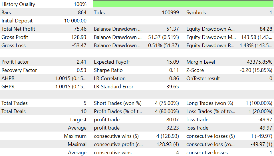
Fig. 4. Strategy Tester report, EURUSD, M30, July 2026. Five trades, profit factor 2.41, maximum equity drawdown 1.43%.
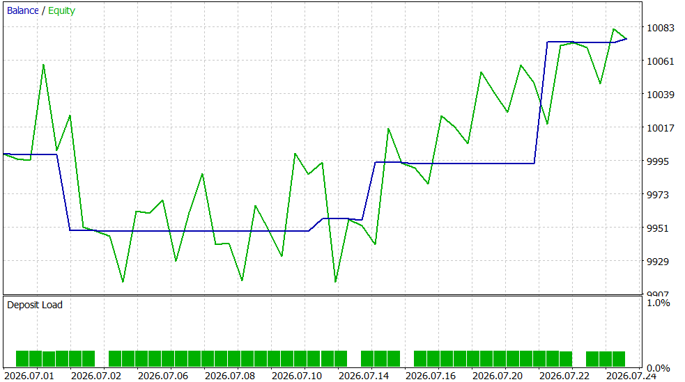
Fig. 5. Equity curve, EURUSD. The balance steps up as the reverse-and-flat logic works through the daily signals.
Over the window the EURUSD run took five trades, four of them short, and closed with a net profit of 75.46 on the 10,000 deposit. The profit factor was 2.41, gross profit against gross loss, and eighty percent of trades were winners. The largest loss, a single stop-out, was 49.97, and the maximum equity drawdown over the run was 1.43 percent. The trade log shows the mechanism doing exactly what it should: positions entering at the daily open, a stop-loss exit reversing the book, and a take-profit closing a short cleanly.
The second run, on EURNZD, was more active.
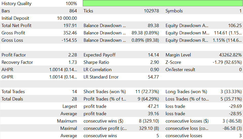
Fig. 6. Strategy Tester report, EURNZD, M30, July 2026. Fourteen trades, profit factor 2.28, maximum equity drawdown 1.15%.
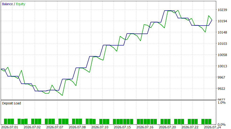
Fig. 7. Equity curve, EURNZD. A longer sequence of consecutive wins builds the balance through the middle of the window.
EURNZD took fourteen trades and closed at a net profit of 197.91, again on the 10,000 deposit. The profit factor was 2.28, close to the EURUSD run, and the maximum equity drawdown was even tighter at 1.15 percent. It strung together a run of eight consecutive wins that accounts for most of the gain, and the balance drawdown never exceeded one percent. Across both symbols the drawdowns stayed under one and a half percent of equity, and both profit factors sat comfortably above two, which is an encouraging early read: the trades the engine produces are coherent, and on this window they were profitable with controlled risk.
Conclusion
We set out to build a trend-follower that does not look at one chart at a time, and we did it entirely in MQL5. Starting from the idea of momentum spillover, we implemented the full network-momentum pipeline from a research paper: volatility-scaled returns, six-speed momentum oscillators, Derivative Dynamic Time Warping to detect who leads whom, a convex graph-learning step to distil those relationships into a sparse weighted network, and propagation of momentum along that network into a single signal per symbol. The whole thing computes its own signal live, with no external solver and no pre-computed data.
- The network is the point. The value over an ordinary MACD is that a leader market's momentum contributes to the signal of the laggers it leads, weighted by a learned connection strength, rather than each market being read in isolation.
- Determinism was engineered in. The DTW tie-breaking and the projected-gradient solver were both chosen so the pipeline produces the same, reproducible output every run, which is what makes a learned-graph strategy trustworthy rather than a source of run-to-run noise.
- Convexity made a pure-MQL5 solver possible. Because the graph-learning objective has a single global optimum, a simple deterministic method reaches the same answer a heavyweight conic solver would, with no dependency on any external library.
- The live bridge is where the real work hides. Date-intersecting a multi-asset universe, caching the expensive graph, and gating execution on the session schedule are what turn a correct signal into a placed trade.
- The results demonstrate the machine, not an edge. Two short tester runs confirm the pipeline works end to end and trades coherently; a durable edge would need long, broad backtesting and forward testing.
The natural next steps are to run the strategy across its whole tradeable forex universe over several years, to restore the paper's continuous volatility-target sizing in place of the fixed pip stops, and to forward-test on a demo account. Each of those builds directly on the frozen, self-contained engine assembled here.
Getting the Source Code via MQL5 Algo Forge
All source files are attached to this article below, but the full repository is also available on MQL5 Algo Forge, the community's Git-based platform for sharing and collaborating on trading projects.
| File name | Description |
|---|---|
| MQL5\Include\NetworkMomentum\NM_Config.mqh | Numeric constants of the pipeline: volatility window, speeds, alpha, beta, lambda, and the ensemble windows |
| MQL5\Include\NetworkMomentum\NM_Matrix.mqh | Row-major matrix type over a double array |
| MQL5\Include\NetworkMomentum\NM_Data.mqh | Volatility scaling: scaled deltas, scaled prices, and the volatility estimate |
| MQL5\Include\NetworkMomentum\NM_Momentum.mqh | Six-speed EMA oscillators and the reverting-sigmoid response function |
| MQL5\Include\NetworkMomentum\NM_DDTW.mqh | Derivative Dynamic Time Warping: the lead-lag matrix V |
| MQL5\Include\NetworkMomentum\NM_GraphLearner.mqh | Convex graph-learning solver for the adjacency matrix A, and symmetric normalisation |
| MQL5\Include\NetworkMomentum\NM_Engine.mqh | Ensemble over windows, propagation, and the final per-symbol signal |
| MQL5\Include\NetworkMomentum\NM_Symbols.mqh | The network universe, resolved against the broker's symbols, and pip sizing |
| MQL5\Include\NetworkMomentum\NM_Live.mqh | Live bridge: gathering and date-aligning D1 bars, and caching the graph |
| MQL5\Experts\NetworkMomentum\NM_Native.mq5 | The Expert Advisor: computes the network-momentum signal and trades it |
Warning: All rights to these materials are reserved by MetaQuotes Ltd. Copying or reprinting of these materials in whole or in part is prohibited.
This article was written by a user of the site and reflects their personal views. MetaQuotes Ltd is not responsible for the accuracy of the information presented, nor for any consequences resulting from the use of the solutions, strategies or recommendations described.

 Neural Networks in Trading: An End-to-End Multivariate Time Series Forecasting Model (GinAR)
 A Reusable Breakeven Manager in MQL5 with Spread Compensation
 Deterministic Dendritic Cell Algorithm (dDCA)
 Quantum Computing and Gradient Boosting in EURUSD Trading

- Free trading apps
- Over 8,000 signals for copying
- Economic news for exploring financial markets
You agree to website policy and terms of use
The cross-market lead-lag approach is interesting, particularly the attempt to translate the network relationship into a fully implementable MQL5 EA. I would be interested in how the lead-lag structure and model parameters are validated out of sample after the network has been constructed. In particular, separating parameter selection from the final untouched OOS period and including spread, commission, and slippage assumptions seems important when assessing whether the observed momentum spillover is robust.