Neural Networks in Trading: An End-to-End Multivariate Time Series Forecasting Model (GinAR)

Introduction

Multivariate time series forecasting (MTSF) has become an integral part of analysis across various industries — from transportation and environmental science to, of course, financial markets. In our field, this means the ability to predict the behavior of several interrelated financial instruments (stocks, indices, currencies) based on their historical dynamics. These models make it possible to make more informed investment decisions, manage risks, and identify hidden relationships between assets.

Formally, a multivariate time series (MTS) can be represented as a spatiotemporal graph, where each variable (whether an exchange rate, trading volume, or rate of return) is observed over time and related to other variables through hidden dependencies. These dependencies fall into two key categories: temporal (cause-and-effect relationships between events) and spatial (interdependencies between assets or market sectors).

For effective MTS forecasting, it is vital to be able to identify and use these spatiotemporal dependencies. This is particularly critical in conditions of high volatility and market shocks, when traditional models simply cannot adapt quickly enough. This is where graph neural networks come to the rescue. These models combine the advantages of graph convolutional networks and recurrent models, enabling more accurate predictions based on complex relationships between variables.

But in practice, things are not quite so straightforward. Financial data are often incomplete. Some metrics are unavailable or are observed for only part of the time interval. Missing values can be caused by anything: disruptions in data delivery, changes in indicator calculation methodologies, or technical errors on the part of brokers. And if data for key assets are missing, forecast accuracy drops sharply. In such cases, graph models typically lose their ability to adequately assess dependencies, which leads to a snowballing accumulation of errors and a decline in forecast quality.

Some attempts to get around this problem are based on simply excluding unavailable variables. But this is short-sighted — the lack of data on a key asset can undermine the entire logical structure of the model and lead to erroneous conclusions. More sophisticated approaches use methods for filling in missing values (imputation), combining temporal context with fixed spatial relationships, such as correlations or network structures among assets. However, such methods often fail when there is a high percentage of missing data or when there are no reliable relationships between the observed and missing variables. And once again, errors accumulate, and the forecast becomes unreliable.

So what should we do? The solution lies in building models capable of using information about available variables to impute missing data directly during the forecasting process, without dividing training into separate “Imputation → Forecasting” stages. This is exactly how the new Graph Interpolation Attention Recursive Network (GinAR) framework works, as presented in the article “GinAR: An End-To-End Multivariate Time Series Forecasting Model Suitable for Variable Missing”. This is a new end-to-end architecture designed to handle missing variables in multivariate time series.

GinAR is based on a simple recurrent network (SRU) that incorporates two key components:

1. Interpolation Attention (IA) is a mechanism that infers missing variables by applying attention algorithms to the available data. This helps avoid errors caused by trying to learn from zeros and outliers.
2. Adaptive Graph Convolution (AGCN) is an adaptive graph convolution that rebuilds the structure of relationships between variables after imputation, allowing it to account for both direct and indirect correlations between assets.

Thus, GinAR simultaneously predicts and refines the dependency model, preventing errors from multiplying. And what's especially important is that it works even under extreme conditions. In tests using real-world data conducted by the framework's authors, the model maintained high accuracy even when up to 90% of the variables were unavailable. Imagine a situation where you only have data for a few assets in your portfolio, while the rest are silent — GinAR still generates a forecast for the entire system.

In short, the key achievements of GinAR are:

• This is the first model designed for MTSF with missing variables that operates without a preliminary imputation step.
• The new architecture (IA + AGCN) replaces the fully connected layers in SRU, minimizing distortions in dependencies.
• According to the experimental results presented in the authors' article, GinAR outperformed 11 other models on five different datasets, demonstrating robust performance even at critically high missingness rates.

For financial markets, this means only one thing: even with some data missing, it is possible to make systematic and accurate forecasts. This means that adaptive strategies, stress tests, and risk management can be implemented reliably without relying on ideal input data. After all, in reality, the market is never perfect — and GinAR was created precisely to be used in such conditions.

GinAR Algorithm

The architecture of the GinAR framework follows the classic Encoder → Decoder scheme. A stack of GinAR layers is used as the Encoder, while the Decoder is implemented using a multilayer perceptron (MLP). A key component of the system is the GinAR cell— a module based on the principle of recursive modeling. When fed incomplete data — that is, time series with missing variables — the model is capable of forecasting future values for all variables simultaneously, even those for which a complete history is missing.

When designing the internal logic of GinAR, the framework’s authors proposed replacing all fully connected layers in the classic recursive structure of SRU with two specialized components: IA (Interpolation Attention) and AGCN (Adaptive Graph Convolution Network).

The first component imputes missing variables using information from available neighbors. This is particularly important in the context of financial markets: if data for key assets are missing, even partially, the model can lose a significant amount of accuracy. The IA mechanism prevents this by reconstructing meaningful representations of the missing time series based on the available data and minimizing the impact of noise.

The second component, AGCN, moves away from fixed dependency graphs, such as predefined relationships between assets, indices, and sectors, and learns an adaptive graph structure directly during training. This makes it possible to flexibly capture spatial relationships between variables, even if they change over time or are not immediately obvious.

The encoder of GinAR is implemented using a recursive scheme in which, at each time step, the current features and the internal state from the previous step are fed as inputs. The GinAR cell processes them, updates the state, and generates a hidden representation of the current time step. This approach makes it possible to simultaneously impute missing data, reconstruct the dependency graph, and extract dynamic patterns — all within a single module. Thanks to residual connections (skip connections), the model can be deep without sacrificing training stability. This is particularly important when predicting complex market signals, where both short-term fluctuations and long-term trends are significant.

The next step is forecasting. To do this, the resulting latent representations must be aggregated correctly. On the one hand, each final hidden state of a GinAR cell contains complete information about the temporal structure of the input data — this is due to the model’s recursive nature. On the other hand, thanks to its multilayer structure and the presence of skip connections, each hidden representation reflects different levels of abstraction: from micro-movements to global correlations. Therefore, the features from all layers are combined into a single tensor and fed into the decoder. The decoder is a multilayer perceptron trained using the Direct Multi-Step Forecasting (DMSF) strategy — a direct multi-step forecasting approach. This approach makes it possible to forecast the entire target horizon at once (for example, price movements over the next 5–10 bars) without resorting to step-by-step iterative forecasting, which is prone to the accumulation of errors.

As a result, GinAR provides a robust architecture capable of effectively handling forecasting tasks in the presence of missing data, dynamic relationships, and high correlation among time series. The model combines missing-data imputation, graph learning, and forecasting — all in a single end-to-end solution capable of adapting to real-world market uncertainty.

The Interpolation Attention (IA) mechanism is designed to reconstruct representations of variables with completely missing historical data. For each missing variable, it is necessary to determine the set of observed variables on which the reconstruction will be based, as well as the corresponding influence weights for these variables. This process consists of two key stages: first, correspondences are established between the missing and available variables, and then an attention mechanism is applied to aggregate information and perform reconstruction.

In the first stage, a correspondence matrix between variables is constructed. An identity matrix IN ∈ Rᴺ*ᴺ is initialized, along with two matrix embeddings of the variables: EIA1 ∈ Rᴺ*ᵈ and EIA2 ∈ Rᵈ*ᴺ. These embeddings are learned jointly with the model. The correlation matrix between variables is computed using the following formula:

The element (i, j) of the matrix AIA ∈ Rᴺ*ᴺ reflects the degree of relationship between variables i and j. If the value is positive, this indicates that the observed variable j can be used to impute the missing variable i. Thus, for each missing variable i, we can identify a set of associated observed variables N(i) ⊆ {1,…,N}.

After the correspondences have been identified, the representations of the missing variables are reconstructed using attention mechanisms. To do this, the attention coefficients aij are computed, reflecting the importance of the observed variable j in reconstructing variable i:

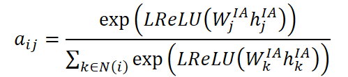
where hᴵᴬj is the current hidden representation of variable j, and Wᴵᴬj is the trainable weight matrix. Activation is performed via the LReLU function, which helps prevent gradients from being zeroed out for weak activations.

The resulting coefficients are used to aggregate information from observed variables. The representation of the missing variable i is reconstructed using the formula:

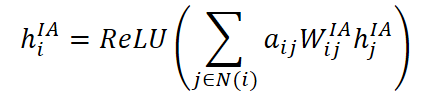
where Wᴵᴬij is a separate trainable weight matrix for each pair of variables i and j, and the final aggregation is normalized using ReLU to improve robustness to outliers.

This process is repeated for all missing variables until the representations for all M missing components have been reconstructed. This results in a new tensor XᴵᴬM ∈ Rᴺ*ᴴ*ᶜ′, in which all variables, including those previously missing, have complete hidden representations. It should be noted that, in practice, steps 2 and 3 are implemented using matrix multiplication and parallel computations to make reconstructing representations more efficient.

Thus, the Interpolation Attention mechanism makes it possible to flexibly impute data in multivariate time series with missing variables, without having to rigidly specify the structure of relationships between variables in advance. This is particularly important for financial forecasting tasks, where the correlation structures among assets can be volatile and historical data may be incomplete or noisy.

In multivariate time series forecasting problems, a predefined graph structure is often used to reflect spatial dependencies between variables. To do this, the adjacency matrix A is defined, which allows the model to capture the underlying relationships. However, with a significant amount of missing data, especially when complete information is lacking for a number of variables, such a predefined graph structure may be insufficient. To overcome this limitation, the framework’s authors have introduced adaptive graph convolution, which combines a predefined structure with a graph generated from the data.

The basis for the predefined graph structure is either distance information (for example, for transportation networks) or the Pearson correlation coefficient between variables, if the data do not contain information about topology. In this case, the adjacency matrix for graph convolution is computed as follows:

where IN ∈ Rᴺ*ᴺ is the identity matrix, D is the degree matrix of the graph vertices, and A is the original adjacency matrix. This normalization helps stabilize the weight scale during training.

However, when some variables are missing or their relationships are unknown, spatial dependencies must be identified dynamically. To this end, an adaptive graph is constructed and learned from the data. This process begins with the initialization of an identity matrix IN ∈ Rᴺ*ᴺ and the random initialization of the variable embeddings EA ∈ Rᴺ*ᵈ. These embeddings are updated as the model is trained.

After imputing the variables using the IA mechanism, we obtain the tensor of hidden representations XᴵᴬM ∈ Rᴺ*ᴴ*ᶜ′. Next, an updated representation of the variables, En ∈ Rᴺ*ᵈ, is computed, combining both embeddings and temporal representations:

where Wx and We are the trainable weight matrices for temporal features and embeddings, respectively, and concat(⋅) is the concatenation operation along the last axis. This representation is used to construct an adaptive adjacency matrix:

The final step is to aggregate information from both graphs using adaptive graph convolution, which combines two channels: one uses a predefined structure, and the other uses an adaptive one. The final representation of the variables is calculated using the following formula:

This design enables the integration of static and dynamic spatial information, which is particularly important when forecasting multivariate time series with partially missing variables.

By combining the two graphs, the model obtains a robust and adaptive structure that enables it to identify dependencies between variables more accurately and, as a result, improve the accuracy of short- and medium-term forecasting.

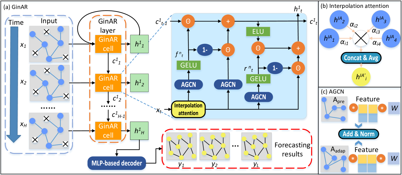
The main idea behind the GinAR architecture is to integrate an interpolation attention (IA) mechanism and adaptive graph convolution (AGCN) into a simple recursive model. This combination makes it possible not only to impute missing variables but also to effectively account for spatiotemporal dependencies.

Let us take a detailed look at the structure of a GinAR cell and the step-by-step process of forecasting the data.

At the level of a single time step, a GinAR cell serves as the basic computational unit. It uses IA to impute missing input values and AGCN to handle spatial relationships between variables. The input is a tensor xT, which is first transformed using the interpolation attention mechanism:

Next, the forget gate fT and reset gate rT are computed by aggregating information from the predefined graph Apre and the adaptive graph Aadapt:

The new state cT is formed as a combination of the current transformed input and the previous state cT-1, weighted by the forget gate:

Finally, the hidden state hT is computed through a nonlinear combination of the updated cell state and the input:

Thus, each GinAR cell performs a complete cycle of updating its internal states, including data imputation and the aggregation of spatial information.

At the global level, the GinAR Encoder consists of several GinAR layers. Each layer consists of H cells connected in series. The original input data X ∈ Rᴺ*ᴴ*ᶜ are first normalized and masked, forming the tensor XM ∈ Rᴺ*ᴴ*ᶜ, where the values of the M variables are zeroed out.

Next, XM is fed into the first GinAR layer, in which each cell is responsible for processing a single time step. The process begins with the initialization of the state c₀, after which x₁ and c₀ are passed to the first cell, producing h¹₁ and c₁. These values are then passed on to the next cell along with x₂, and so on. The result is a sequence of hidden states of the first layer, h¹ = [h¹₁, h¹₂, …, h¹H].

This tensor serves as the input for the next layer. The process is repeated until all n layers have been processed. Then the last hidden state hHⁱ is extracted from each layer, and they are concatenated into the final vector halln.

The final representation halln is fed into a decoder based on a multilayer perceptron (MLP), which generates forecast values:

Thus, GinAR implements full end-to-end processing of time series with missing values, combining data imputation and the modeling of spatiotemporal dependencies within a single recursive-convolutional framework.

The authors’ visualization of the GinAR framework is shown below.

Implementation in MQL5

After reviewing the theoretical aspects of the GinAR framework, we move on to the practical section, where we will demonstrate one way to implement the approaches described by the framework’s authors using MQL5.

However, before we begin developing the main algorithm, we need to do some preparatory work. As can be seen from the above description of GinAR, the original algorithm repeatedly applies data normalization using the SoftMax function. In light of this, we decided to implement it as a separate function in the OpenCL program, thereby ensuring flexibility and high performance when working with multivariate data.

Preparatory Work

For better organization, we have broken down the implementation of the algorithm into separate functional blocks. Let's start with the first one: finding the maximum value among the threads in a work-group. The LocalMax function performs this task.

The LocalMax function takes two parameters: the value computed in the current thread and the dimension index in the task space (loc) by which threads are grouped into work-groups.

#define BarrierLoc      barrier(CLK_LOCAL_MEM_FENCE)
float LocalMax(const float value, const int loc)
  {
   const size_t id = get_local_id(loc);
   const size_t total = get_local_size(loc);
//---
   __local float Temp[LOCAL_ARRAY_SIZE];
   const uint ls = min((uint)total, (uint)LOCAL_ARRAY_SIZE); 

In the first step, the thread ID within the local work-group and the total size of the work-group are determined. Next, a Temp array is created and stored in the device's local memory; this array will be used to exchange intermediate values between threads within the same work-group.

Then the program begins iterating through all the subgroups formed within the work-group in order to find local maxima. The values are stored in the elements of the Temp array.

//--- Find Max
   for(int d = 0; d < total; d += ls)
     {
      if(id >= d && id < (d + ls) &&
         (d == 0 || Temp[id - d] < value))
         Temp[id - d] = IsNaNOrInf(value, MIN_VALUE);
      BarrierLoc;
     }

After that, an iterative process of reduction (collapsing) starts, reducing the Temp array to a single value — the maximum among all its elements.

   int count = ls;
   do
     {
      count = (count + 1) / 2;
      if(id < count && (id + count) < ls && Temp[id] < Temp[id + count])
         Temp[id] = Temp[id + count];
      BarrierLoc;
     }
   while(count > 1);
//---
   return IsNaNOrInf(Temp[0], MIN_VALUE);
  }

The result of these operations is returned to the calling program.

Similar to the previous LocalMax function, let's create another basic building block — a function for summing elements within a local work-group. This task is performed by the LocalSum function, which is based on the same principle as LocalMax, but uses addition instead of finding a maximum.

float LocalSum(const float value, const int loc)
  {
   const size_t id = get_local_id(loc);
   const size_t total = get_local_size(loc);
//---
   __local float Temp[LOCAL_ARRAY_SIZE];
   const uint ls = min((uint)total, (uint)LOCAL_ARRAY_SIZE);

In the initial stage, as before, the thread identifier and the size of the work-group are determined. A local Temp array is also created to store intermediate sums.

Next comes iteration over all threads in the local work-group, accumulating intermediate values. Note the use of the condition d == 0, which ensures that the Temp array is initialized correctly on the first iteration.

//--- Sum
   float result = IsNaNOrInf(value, 0);
   for(int d = 0; d < total; d += ls)
     {
      if(id >= d && id < (d + ls))
         Temp[id - d] = (d == 0 ? result : Temp[id - d] + result);
      BarrierLoc;
     }

After that, the familiar reduction process is performed, with the number of elements halved at each step; here, instead of a comparison, the elements of the Temp array are simply summed.

   int count = ls;
   do
     {
      count = (count + 1) / 2;
      if(id < count && (id + count) < ls)
         Temp[id] += Temp[id + count];
      BarrierLoc;
     }
   while(count > 1);
   result = IsNaNOrInf(Temp[0], 0);
//---
   return result;
  }

The final value, the sum of all elements in the work-group, is returned to the calling program.

At the final stage of the preparatory work, we will combine the previously implemented auxiliary functions LocalMax and LocalSum into a single algorithm for the LocalSoftMax function, which performs numerically stable normalization of values within a work-group.

float LocalSoftMax(const float value, const int loc)
  {
//--- Look Max
   const float max = LocalMax(value, loc);
   BarrierLoc;

Inside the LocalSoftMax function, LocalMax is called first; it finds the maximum value among all threads in the work-group. This is necessary to stabilize the calculations: subtracting the maximum from each value prevents overflow and improves the numerical stability of exponential operations.

Then, with the shift applied, the exponential of each value is computed. The result of this operation is temporarily stored in the variable result, after which we call the LocalSum function to calculate the total sum of the exponentials within the group.

//--- SoftMax
   float result = IsNaNOrInf(exp(value - max), 0);
   const float sum = LocalSum(result, loc);
   result = IsNaNOrInf(result / (sum == 0 ? 1 : sum), 0);
//---
   return result;
  }

Next, normalization is performed: the value result is divided by the sum of all the exponentials. In addition, protection against division by zero is provided: if the sum is zero, one is used in the denominator. As a final step, we return the normalized value.

This structure allows SoftMax to be used as a flexible building block for subsequent OpenCL kernels. This makes the code cleaner, simplifies debugging, and improves the readability of the entire architecture, especially in the context of graph models and attention mechanisms used in the GinAR implementation in MQL5.

However, a forward pass through SoftMax alone is still not enough to train the model. To update the weights correctly during backpropagation, the appropriate gradient propagation function must be implemented. This function allows the model to account for how a change in the input value will affect the final error.

We implement this functionality in the LocalSoftMaxGrad function, which determines the gradient of the SoftMax function with respect to the input value. The input parameters are: the value value, corresponding to the output of SoftMax; the gradient grad, passed from a later layer of the network; and the task-space dimension index loc, according to which work-groups are formed.

float LocalSoftMaxGrad(const float value, const float grad, const int loc)
  {
   const size_t id = get_local_id(loc);
   const size_t total = get_local_size(loc);
//---
   __local float Temp[LOCAL_ARRAY_SIZE];
   const uint ls = min((uint)total, (uint)LOCAL_ARRAY_SIZE);

At the beginning of the function, we determine the ID of the current thread and the total number of threads in the local work-group. We create a local array Temp to store intermediate values, similar to how this was done in LocalMax and LocalSum. The variable val is an error-protected input value.

   float result = 0;
   float val = IsNaNOrInf(value, 0);
   for(uint d = 0; d < total; d += ls)
     {
      if(id >= d && id < (d + ls))
         Temp[id - d] = IsNaNOrInf(val * grad, 0);
      BarrierLoc;
      for(uint l = 0; l < min(ls, (uint)(total - d)); l++)
         result += Temp[l] * ((float)((d + l) == id) - val);
      BarrierLoc;
     }
//---
   return result;
  }

Next, we start iterating over the subgroups within the entire work-group. In each block, we fill the temporary buffer with the values of the product val * grad and, using the standard formula for the derivative of SoftMax, accumulate the result in the variable result. The expression itself uses the logical check (d + l) == id, which ensures that both diagonal and off-diagonal elements of the Jacobian are processed correctly.

The result of the function is the final gradient value corresponding to the given input element. This result is returned to the calling kernel, ensuring that the backward pass is implemented correctly in the model architecture.

Thus, this function completes the implementation of the full SoftMax processing cycle within the OpenCL module — from the forward computation to proper gradient backpropagation.

Interpolation Attention

After completing the preparatory work related to implementing basic operations, such as SoftMax and the propagation of its gradient, we move on to building the Interpolation Attention mechanism, which plays a key role in the GinAR architecture. In the first stage, our goal is to implement the forward pass of this algorithm using OpenCL, ensuring efficient parallel processing on the graphics accelerator.

As input, the InterpositionAttention kernel takes several arrays:

• the input feature matrix matrix_in,
• trainable parameters W and A,
• latent representations GL,
• adjacency matrices Adj,
• intermediate representations H,
• attention values Atten,
• the resulting matrix matrix_out.

The feature-space dimension is also provided.

__kernel void InterpositionAttention(__global const float* matrix_in,
                                     __global const float* W,
                                     __global const float* A,
                                     __global const float* GL,
                                     __global float* Adj,
                                     __global float* H,
                                     __global float* Atten,
                                     __global float* matrix_out,
                                     const int dimension
                                    )
  {
   const size_t i = get_global_id(0);
   const size_t j = get_local_id(1);
   const size_t total = get_global_size(0);
   const size_t total_loc = get_local_size(1);

At the start of execution, we define the global and local thread indices i and j, which will be used to iterate over elements in the input and output arrays. Next, we calculate the appropriate offsets to ensure correct access to the subarrays within the global buffer.

const int shift_i = i * dimension;
const int shift_j = j * dimension;
const int shift_adj = i * total_loc + j;

The first step is to calculate the adjacency weights between two nodes, i and j, by pairwise multiplying their latent representations from the GL array.

float adj = 0;
for(int d = 0; d < dimension; d++)
   adj += IsNaNOrInf(GL[shift_i + d] * GL[shift_j + d], 0);
adj = max(IsNaNOrInf(adj, 0), 0);
adj = LocalSoftMax(adj, 1);
Adj[shift_adj] = adj;
adj += (float)(i == j);

The result is accumulated in the variable adj, normalized using the LocalSoftMax function, and stored in the adjacency matrix Adj. Then, one is added to adj if i matches j, thereby ensuring that the diagonal element is preserved.

Next, we proceed to form the intermediate representation H. To do this, the input features of the current node are multiplied step by step by the trainable weight matrix W. Each value is stored in the array H, and the BarrierLoc barrier is used for synchronization between threads.

for(int id_h = 0; id_h < dimension; id_h += total_loc)
  {
   if(j >= (dimension - id_h))
      break;
   float h = 0;
   for(int w = 0; w < dimension; w++)
      h += IsNaNOrInf(matrix_in[shift_i + w] * W[(id_h + j) * dimension + w], 0);
   H[shift_i + id_h + j] = h;
   BarrierLoc;
  }

Once H has been formed, the attention value e is calculated, which determines the importance of the interaction between nodes i and j. The value is initialized to a small positive number to avoid division by zero. If there is a positive correlation between the elements, the weighted dot products between the corresponding rows of H and the trainable vector A are accumulated. The result is normalized again using the LocalSoftMax function and stored in the Atten array.

float e = 1e-12f;
if(adj > 0)
  {
   e = 0;
   for(int a = 0; a < dimension; a++)
      e += IsNaNOrInf(H[shift_i + a] * A[a], 0) + IsNaNOrInf(H[shift_j + a] * A[dimension + a], 0);
  }
e = LocalSoftMax(e, 1);
Atten[shift_adj] = e;

The final step is to impute the value of the variable under analysis based on information obtained from other observed variables. The value of the missing (or to-be-imputed) variable i is aggregated through a weighted sum of the representations of variables j, with the representations themselves multiplied by the corresponding attention coefficients. This type of aggregation allows useful information to be passed from neighbors to the target variable.

 for(int d = 0; d < dimension; d += total_loc)
   {
    if(j >= (dimension - d))
       break;
    float out = 0;
    int shift_h = d + j;
    int shift_att = i * total_loc;
    int shift_out = i * dimension + shift_h;
    for(int n = 0; n < total_loc; n++)
       out += IsNaNOrInf(H[shift_h + n * dimension] * Atten[shift_att + n], 0);
    matrix_out[shift_out] = Activation(out, ActFunc_LReLU);
   }
}

To improve robustness to outliers and mitigate the impact of anomalous values, the resulting value is normalized using the LReLU activation function. This helps ensure more stable model training, especially when dealing with an unstable or noisy dataset.

This step completes the forward pass of Interpolation Attention and forms the final representation of variable i, taking into account both the internal relationships between variables and the learned correlation parameters.

Thus, the OpenCL kernel described here implements the forward pass of Interpolation Attention, effectively leveraging parallelism to process the elements of the graph structure. It enables the construction of an adaptive model of interactions between elements in a time series based on latent features, which allows for context to be taken into account and for the model to adapt flexibly to the data structure.

The next step in our work is to implement the backward pass algorithm for Interpolation Attention, which we will also package as an OpenCL kernel. This function calculates the gradients for all parameters and input data involved in the forward pass.

The main idea behind the code is to compute, for each element, the partial derivatives of the error with respect to the intermediate variables: the hidden features H, the attention coefficients Atten, the input matrices, the weights, and the feature matrix GL.

__kernel void InterpositionAttentionGrad(__global const float* matrix_in,
                                         __global float* matrix_in_gr,
                                         __global const float* W,
                                         __global float* W_gr,
                                         __global const float* A,
                                         __global float* A_gr,
                                         __global const float* GL,
                                         __global float* GL_gr,
                                         __global float* Adj,
                                         __global float* H,
                                         __global float* H_gr,
                                         __global float* Atten,
                                         __global float* matrix_out_gr,
                                         const int dimension
                                        )
  {
   const size_t i = get_global_id(0);
   const size_t j = get_local_id(1);
   const size_t total = get_global_size(0);
   const size_t total_loc = get_local_size(1);

Inside the kernel, for each thread (identified by indices i and j), the following sequential computation takes place:

• The gradients with respect to the hidden features, Hgrad, are computed from the output gradients and the attention weights, taking into account the LeakyReLU activation function.

   const int shift_i = i * dimension;
   const int shift_j = j * dimension;
   const int shift_adj = i * total_loc + j;
//--- H Gradient
   for(int d = 0; d < dimension; d += total_loc)
     {
      if(j >= (dimension - d))
         break;
      float h_grad = 0;
      int shift_h = shift_i + d + j;
      int shift_att = i;
      int shift_out = d + j;
      for(int n = 0; n < total_loc; n++)
        {
         float gr = matrix_out_gr[shift_out + n * dimension];
         h_grad += IsNaNOrInf(
                      Deactivation(gr, gr, ActFunc_LReLU) * Atten[shift_att + n * total_loc], 0);
        }
      H_gr[shift_h] = h_grad;
      BarrierLoc;
     }

• Next, the gradient with respect to the attention coefficients, Attgrad, is calculated and passed through the SoftMax backward pass to ensure proper error propagation in the attention distribution.

//--- Attention Gradient
   float att_grad = 0;
   for(int d = 0; d < dimension; d++)
     {
      float gr = matrix_out_gr[shift_i + d];
      gr = Deactivation(gr, gr, ActFunc_LReLU);
      att_grad += IsNaNOrInf(gr * H[shift_j + d], 0)
     }
   att_grad = LocalSoftMaxGrad(Atten[shift_adj], att_grad, 1);

• This gradient is then used to update the gradients with respect to the hidden features H, taking into account the weights in matrix A, as well as to accumulate the gradients with respect to matrix A itself.

for(int d = 0; d < dimension; d++)
  {
   float h_grad = att_grad * A[d];
   h_grad = LocalSum(h_grad, 1);
   if(j == 0)
      H_gr[shift_i + d] += h_grad;
   h_grad = att_grad * A[dimension + d];
   h_grad = LocalSum(h_grad, 1);
   if(j == 0)
      H_gr[shift_j + d] += h_grad;
   float a_grad = att_grad * H[shift_i + d];
   a_grad = LocalSum(a_grad, 1);
   A_gr[d] += a_grad;
   a_grad = att_grad * H[shift_j + d];
   a_grad = LocalSum(a_grad, 1);
   A_gr[dimension + d] += a_grad;
  }

• The gradients with respect to the input features are obtained using the gradients of the hidden features and the weight matrices W, which allows the input data to be correctly updated during training.

//--- Input Gradient
   for(int d = 0; d < dimension; d += total_loc)
     {
      if(j >= (dimension - id_h))
         break;
      float grad = 0;
      for(int w = 0; w < dimension; w++)
         grad += IsNaNOrInf(H_gr[shift_i + w] * W[(id_h + j) + dimension * w], 0);
      matrix_in_gr[shift_i + d + j] = grad;
      BarrierLoc;
     }

• Finally, the gradients with respect to the adaptive matrix GL are computed via the SoftMax backward pass over the adjacency matrix and are accumulated for both variables i and j.

//--- Adj Gradient
   float grad = LocalSoftMaxGrad(Adj[shift_adj], att_grad, 1);
   for(int d = 0; d < dimension; d++)
     {
      GL_gr[shift_i + d] += IsNaNOrInf(grad * GL[shift_j + d], 0);
      GL_gr[shift_j + d] += IsNaNOrInf(grad * GL[shift_i + d], 0);
     }
  }

The overall structure of the function is built using local thread synchronization (BarrierLoc), which ensures the correctness of data exchange between threads and prevents race conditions.

This approach ensures accurate and stable updates to all model parameters during training, enabling effective adjustment of weights and improving the quality of missing-value imputation in multivariate time series.

At this stage, we complete the implementation of the key components in the OpenCL program. The next logical step will be to organize the entire process within the main program — integration, computation management, and model training using MQL5 tools. However, the amount of material has already grown significantly, and to maintain clarity and the quality of the presentation, I suggest we take a break.

We will continue this important work in the next article, where we will discuss in detail the practical implementation of the algorithm in MQL5, the specifics of interacting with OpenCL, and performance optimization. That way, we can focus on each stage without rushing, while maintaining the depth and thoroughness of our exploration of the topic.

Conclusion

In conclusion, it is worth emphasizing that the GinAR framework presented here demonstrates a powerful approach to forecasting multivariate time series with missing values. The integration of interpolation attention and adaptive graph convolution into a recursive architecture enables effective imputation of missing data and accounts for complex spatiotemporal dependencies.

The practical implementation of the key components in OpenCL, as presented in this article, opens up a wide range of opportunities for further optimization and integration into real-world trading systems.

Future work will focus on integrating these developments into the main program in MQL5, which will allow us to realize the full potential of the proposed methods. I invite readers to continue exploring this topic in the next article.

References

• GinAR: An End-to-End Multivariate Time Series Forecasting Model Suitable for Variable Missing
• Other articles in this series

Programs used in the article

#	Name	Type	Description
1	Study.mq5	EA	Expert Advisor for offline model training
2	StudyOnline.mq5	EA	Expert Advisor for online model training
3	Test.mq5	EA	Expert Advisor for model testing
4	Trajectory.mqh	Class Library	Structure describing the system state and model architecture
5	NeuroNet.mqh	Class Library	Class library for building a neural network
6	NeuroNet.cl	Library	Code library for an OpenCL program