Neural Networks in Trading: Adaptive Periodic Segmentation (Conclusion)

Introduction

In previous articles, we took a step-by-step look at how the LightGTS framework converts time series into musical scores. First, in the Period Patching module, the data being analyzed is automatically divided into complete cycles determined using the FFT. Each such cycle is then projected into a token using the Flex Projection Layer, which enables flexible processing of fragments of varying lengths. In the Encoder, these tokens are enriched with Rotary Positional Encoding (RoPE) — a compact way to weave in phase shifts and relative positions — after which classic Transformer blocks with multi-head attention fuse local patterns into a unified context. The forecast is generated using the Periodical Parallel Decoding mechanism, which instantly produces the entire output sequence without autoregression. The result is adjusted in the Flex-resize module, which preserves periodic consistency.

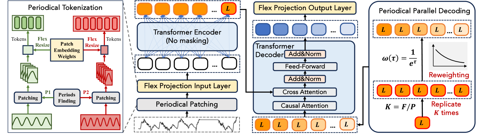
By this point, we had already successfully implemented the key ideas of LightGTS in code: we had learned how to automatically slice a time series into periodic segments using adaptive patching and convert each segment into an informative token. We added our own touches to the original algorithms, refined the logic behind flexible projection, and obtained ready-to-use representations of local market cycles. Today, we'll take the next step toward developing our own view of the approaches proposed by the authors of the LightGTS framework.

The RoPE Mechanism

Once the adaptive convolution had extracted a concentrated set of informative tokens from the raw time series, it was time to pass them through the powerful filter of Transformer blocks. In the standard Encoder–Decoder architecture, sinusoidal or learnable positional encoding vectors are simply added to these tokens, after which they are sent to the attention mechanism. The authors of the LightGTS framework propose a much more elegant and flexible approach: Rotary Positional Encoding (RoPE). Instead of fixed positional-encoding vectors, each token is rotated in embedding space.

The main idea behind RoPE is to introduce a vector phase shift proportional to the token’s position and its dimensional indices, without resorting to additional parameters. It should be noted that this technique was first introduced in the paper "RoFormer: Enhanced Transformer with Rotary Position Embedding," in which the authors demonstrated that rotating coordinate pairs of the Query and Key vectors using a rotation matrix allows the model to reliably capture relative temporal shifts.

The method can easily be generalized to multidimensional spaces by splitting the dimensionality into pairs of values. This leads to a constraint: the dimension of the space must be even.

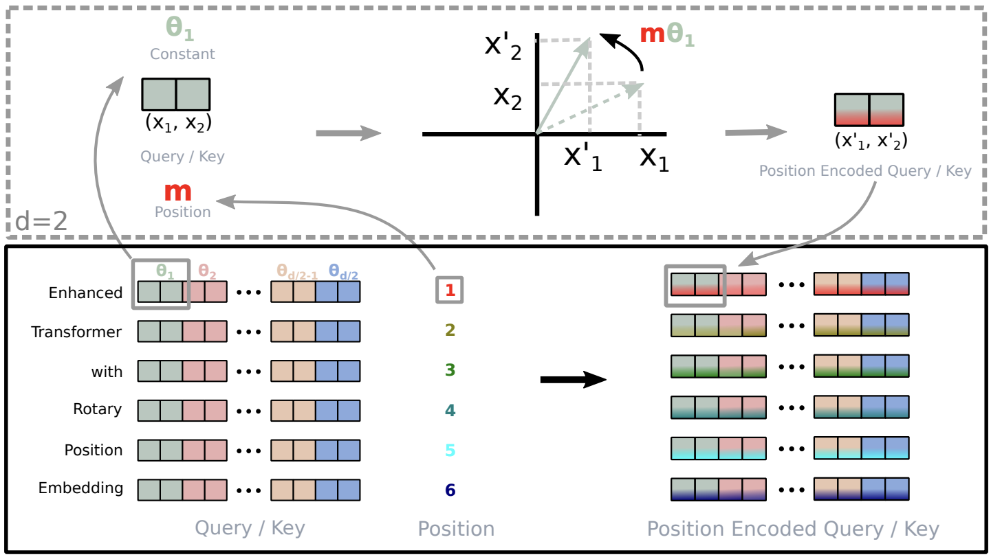
Thanks to this rotation, even with varying window sizes and a dynamic step size, the model accurately determines which tokens are closer in time and which are farther away. As a result, the Self-Attention mechanism becomes a highly sensitive detector of temporal patterns: it does not simply compare the contents of Query and Key, but also takes into account phase differences between tokens. As a result, after several layers of multi-head attention and Feed-Forward, the tokens emerge deeply contextualized.

Now that we have delved into the mathematical and conceptual foundations of Rotary Positional Encoding, it is time to get into the nuts and bolts of the implementation and see how to translate all of this into OpenCL program code. We already have prepared tokens — an array of vectors, each with D dimensions. In addition, we will precompute sine and cosine tables for each position. Our goal is to rotate each vector in the embedding space so that its phase reflects the timestamp, without sacrificing overall pipeline throughput. To do this, we create a RoPE kernel that operates in a three-dimensional task space. The first dimension corresponds to the index of the pair of coordinates within the vector. Its dimension is equal to half the length of the vector. The second dimension indicates the length of the sequence (the number of tokens). The third indicates the number of unit sequences.

Please note that, for convenience when working with pairs of values, we use the float2 vector data type.

__kernel void RoPE(__global const float2* __attribute__((aligned(8))) inputs,
                   __global const float2* __attribute__((aligned(8))) position_emb,
                   __global float2* __attribute__((aligned(8))) outputs
                  )
  {
   const size_t id_d = get_global_id(0);     // dimension
   const size_t id_u = get_global_id(1);     // unit
   const size_t id_v = get_global_id(2);     // variable
   const size_t dimension = get_global_size(0);
   const size_t units = get_global_size(1);
   const size_t variables = get_global_size(2);

In the kernel body, we first identify the coordinates of the current work-item in the three-dimensional task space. This is necessary so that each work-item knows exactly which data fragment it will be working with: which pair of vector coordinates to process, which token it belongs to, and which variable (or channel) it comes from.

Once the work-item coordinates are known, the next step is computing the offsets in the flat arrays of OpenCL buffers. Despite the multidimensional logical structure, all data in OpenCL is stored linearly, so you need to manually calculate the exact memory location of the element of interest.

   const int shift_in = (id_v * units + id_u) * dimension + id_d;
   const int shift_pos = id_u * dimension + id_d;
   const float2 inp = inputs[shift_in];
   const float2 pe = position_emb[shift_pos]; 

To minimize costly accesses to global memory, we immediately load the initial pair of coordinates and the corresponding sine/cosine factors into local vector variables that effectively stay in registers for the kernel. After all, every access to global memory buffers is significantly more expensive than working with vectors already held locally. This almost completely eliminates repeated reads from global memory and keeps hot data in registers or in GPU local memory, which significantly speeds up the entire process of rotating tokens and maximizes kernel execution efficiency.

Once all the ingredients (the input data and the sin/cos values) are at hand, we are ready to move on to the main event — the phase shift. It is this shift that gives tokens a sense of time and ensures that the attention mechanism functions properly.

   float2 result = 0;
   result.s0 = inp.s0 * pe.s0 - inp.s1 * pe.s1;
   result.s1 = inp.s0 * pe.s1 + inp.s1 * pe.s0;
//---
   outputs[shift_in] = result;
  }

Here, we use simple arithmetic operations on local variables: four multiplications and two additions for each pair of values. Thanks to the preloaded data, this step is completed almost instantly.

After that, we immediately write the rotated pair of coordinates to the result buffer.

That's the whole trick: by simply multiplying by precomputed cos and sin values, we give each token information about phase and relative time without adding a single new parameter. As a result, this kernel demonstrates:

• Maximum parallelism — each work-item runs independently.
• Zero training overhead — positional encoding contains no trainable parameters.
• Seamless integration with subsequent attention modules — embeddings account not only for the content of the tokens but also for their phase differences.

Although RoPE does not introduce a single trainable parameter into the model, it is important to us that gradients can flow correctly through this layer and back to the input data. To do this, we create a special backward pass kernel called CalcHiddenGradRoPE, which performs the reverse rotation of the vectors.

The idea is simple: the forward pass kernel multiplied the input data (x, y) by a rotation matrix. In the backward direction, we need to apply its transpose — that is, a rotation by −θ, where cos(−θ) = cosθ and sin(−θ) = −sinθ.

The algorithm for the backward pass kernel is virtually identical to the one discussed above for the forward pass. The same task space is used, and offsets in the global data buffers are defined in a similar manner. The only slight difference lies in the rotation of the vectors. Moreover, the input data for performing the operations are the error gradients at the output level.

__kernel void CalcHiddenGradRoPE(__global float2* __attribute__((aligned(8))) inputs_gr,
                                 __global const float2* __attribute__((aligned(8))) position_emb,
                                 __global const float2* __attribute__((aligned(8))) outputs_gr
                                )
  {
   const size_t id_d = get_global_id(0);     // dimension
   const size_t id_u = get_global_id(1);     // unit
   const size_t id_v = get_global_id(2);     // variable
   const size_t dimension = get_global_size(0);
   const size_t units = get_global_size(1);
   const size_t variables = get_global_size(2);
//---
   const int shift_in = (id_v * units + id_u) * dimension + id_d;
   const int shift_pos = id_u * dimension + id_d;
   const float2 grad = outputs_gr[shift_in];
   const float2 pe = position_emb[shift_pos];
//---
   float2 grad_x;
   grad_x.s0 = grad.s0 * pe.s0 + grad.s1 * pe.s1;
   grad_x.s1 = grad.s1 * pe.s0 - grad.s0 * pe.s1;
//---
   inputs_gr[shift_in] = grad_x;
  }

No conditional branches or complicated formulas — just four multiplications and a couple of additions. As a result, the gradients of the RoPE layer are unwound just as quickly and efficiently as the tokens were rotated during the forward pass.

As a result, CalcHiddenGradRoPE turns the RoPE layer into a full-fledged participant in the training process: we can incorporate it at any depth of the network, and it will return gradients to the input tensors without loss, preserving execution speed and parallelism.

Now that our OpenCL kernels for Rotary Positional Encoding are polished to perfection, it is time to bring this power into the MQL5 world and integrate it with a trading robot. We already have a ready-made mechanism for rotating tokens on the GPU — all that is left is to create a lightweight wrapper around it that fits into the familiar structure of MQL5 Expert Advisors. For exactly this purpose, we will create the CNeuronRoPE class, whose structure is shown below.

class CNeuronRoPE  :  public CNeuronPositionEncoder
  {
protected:
   uint              iWindow;
   uint              iVariables;
   //---
   virtual bool      feedForward(CNeuronBaseOCL *NeuronOCL) override;
   virtual bool      calcInputGradients(CNeuronBaseOCL *NeuronOCL)override;

public:
                     CNeuronRoPE(void) : iWindow(0), iVariables(0) {};
                    ~CNeuronRoPE(void) {};
   //---
   virtual bool      Init(uint numOutputs, uint myIndex, COpenCLMy *open_cl,
                          uint count, uint window, uint variables,
                          ENUM_OPTIMIZATION optimization_type, uint batch);
   //--- methods for working with files
   virtual bool      Save(int const file_handle) override;
   virtual bool      Load(int const file_handle) override;
   //---
   virtual int       Type(void) override const {  return defNeuronRoPE; }
  };

The CNeuronRoPE class is designed to be as simple as possible: it has only two variables: iWindow, which defines the dimensionality of a single token vector, and iVariables, which specifies the number of channels. All the other heavy-duty functionality related to buffers and parameter checking is inherited from CNeuronPositionEncoder, so the constructor and destructor are empty here. The foundation for the entire layer's operation is laid in the Init method.

bool CNeuronRoPE::Init(uint numOutputs, uint myIndex, COpenCLMy *open_cl,
                       uint count, uint window, uint variables,
                       ENUM_OPTIMIZATION optimization_type, uint batch)
  {
   if(window % 2 > 0)
      return false;
   if(!CNeuronBaseOCL::Init(numOutputs, myIndex, open_cl, count * window * variables, optimization_type, batch))
      return false;

At the very beginning of the method, we perform a simple but extremely important check: the dimension of each token must be even, since RoPE operates on pairs of coordinates. Without this constraint, we simply cannot proceed any further: we will not be able to unambiguously rotate pairs of values. Once the checkpoint has been passed successfully, we transfer control to the method of the same name in the parent class, where the remaining checkpoints and the initialization algorithm for the inherited interfaces are already implemented.

Next, we store the parameters of the input data tensor in internal variables.

   iWindow = window;
   iVariables = variables;

Now we move on to constructing the embedding matrix that is key to RoPE: a two-dimensional array where the even columns contain cos(θ) and the odd columns contain sin(θ).

First, we create a pe matrix of the required size. This is a canvas that we will immediately fill with sine and cosine values. To understand how each column of the matrix will respond to its corresponding time-series step, we first construct a position vector: we take a unit vector, compute its prefix sums, and subtract one, resulting in [0, 1, 2, …, count–1]. It is this vector that tells us exactly which step we are currently encoding.

   matrix<float> pe = matrix<float>::Zeros(count, iWindow);
   vector<float> position = vector<float>::Ones(count);
   position = position.CumSum() - 1;

Next comes the main part: we iterate through all pairs of dimensions, since each pair of token coordinates requires its own set of angles. For each such pair, we take the position vector and divide it by a growing denominator equal to pow(10000, 2 * i / iWindow) to slow down the rotation of the higher-order dimensions and speed up the lower-order ones. As a result, we obtain an array of angles: not individual numbers, but a vector θ for all positions.

   for(uint i = 0; i < iWindow / 2; i++)
     {
      vector<float> temp = position / MathPow(10000.0f, 2.0f * i / window);
      pe.Col(MathCos(temp), i * 2);
      pe.Col(MathSin(temp), i * 2 + 1);
     }

And so, into each even column of the pe matrix we write the cosines of the resulting angles, and into the adjacent odd column, the sines. As a result, the matrix becomes a ready-to-use table, where each column is equipped with its own pair of values [cos(θ), sin(θ)], ready to rotate any token. We perform all these calculations once in CPU code so that we can then pass a ready-to-use set of functions to the GPU kernels.

We transfer the filled matrix to the data buffer and complete the method by returning the boolean result of the operations to the calling program.

   PositionEncoder.BufferFree();
   if(!PositionEncoder.AssignArray(pe))
      return false;
   SetActivationFunction(None);
//---
   return PositionEncoder.BufferCreate(open_cl);
  }

Thanks to this approach, our OpenCL kernels receive a precomputed sine/cosine table as input and can operate at full capacity without being distracted by unnecessary mathematical operations.

As a result, all the initial setup is concentrated in a single method: simply change the window or variables parameters, and the layer instantly adapts to the new conditions. This approach ensures that the code remains strict and clear, while giving us full control over the behavior of the RoPE module.

When the forward pass begins, all you need to do is call the feedForward method, passing it a pointer to the source data object that has already been populated with tokens. Under the hood, the method pays close attention to detail: it checks whether the received pointer is valid, queues a RoPE kernel with the appropriate work-group sizes, waits for it to complete, and then returns control. The result is a buffer of rotated tokens, ready to be passed to the attention module.

During training, the calcInputGradients method comes into play. This method launches the CalcHiddenGradRoPE kernel. The logic itself is almost the mirror image of the forward pass: the same coordinates, the same offsets, but the rotation goes in the opposite direction to restore the gradient to its original representation. The final result is neatly placed in the input-gradient buffer and flows smoothly onward to the earlier layers of the model.

Both methods are, in essence, wrappers for the corresponding kernels and follow an algorithm you are already familiar with. Therefore, we will not discuss them in detail in this article. The complete code for the class presented here, along with all of its methods, can be found in the attachment.

Now that the tokens have passed through the RoPE phase filter, they are ready to enter the heart of the model — the attention module. By default, the LightGTS framework builds its logic around the classic Encoder–Decoder architecture, so we do not have to reinvent the wheel: all the necessary components are already available in our library. All you need to do is feed the rotated tokens into one of the existing Self-Attention modules, where multi-head attention will work very effectively, linking local patterns to the global context of the time series.

In the original version of LightGTS, the authors propose taking the last hidden token after the Encoder and replicating it exactly as many times as needed to cover the specified forecast horizon, so that the Decoder can generate the entire output sequence at once. We, on the other hand, took a bold step toward simplification: we don't need replication. First, our goal is not to obtain highly precise figures, but to extract all the valuable information from the latent representation for the Agent, which will use it to make trading decisions. Second, we run calculations on each new bar, which is always shorter than a full market cycle. So, one final token for each unit sequence is quite enough for us.

Therefore, bypassing multiple copies, we route this final embedding through the main pipeline to the Decoder. There, it encounters the same multi-head attention and Feed-Forward, but without unnecessary repetitions: the model relies on a pure, concentrated representation containing all relevant information about the latest market movements. This approach conserves resources, simplifies the logic, and allows the Agent to act as quickly as possible — after all, every bar requires an instant response, and we do not need a thousand copies of a token, but a single powerful signal ready to lead to profit.

Model Architecture

Finally, we arrive at the culmination — the moment when all the carefully debugged modules come together into a single, smoothly functioning system. In our MQL5 project, this takes place in the CreateDescriptions function, where we build the seven branches of the neural network step by step: the Encoder, three predictive streams, and the three components of the Agent — Actor, Director, and Critic.

bool CreateDescriptions(CArrayObj *&encoder,
                        CArrayObj *&forecast1,
                        CArrayObj *&forecast2,
                        CArrayObj *&forecast3,
                        CArrayObj *&actor,
                        CArrayObj *&director,
                        CArrayObj *&critic
                       )
  {
//---
   CLayerDescription *descr;
//---
   if(!encoder)
     {
      encoder = new CArrayObj();
      if(!encoder)
         return false;
     }
   if(!forecast1)
     {
      forecast1 = new CArrayObj();
      if(!forecast1)
         return false;
     }
   if(!forecast2)
     {
      forecast2 = new CArrayObj();
      if(!forecast2)
         return false;
     }
   if(!forecast3)
     {
      forecast3 = new CArrayObj();
      if(!forecast3)
         return false;
     }
   if(!actor)
     {
      actor = new CArrayObj();
      if(!actor)
         return false;
     }
   if(!director)
     {
      director = new CArrayObj();
      if(!director)
         return false;
     }
   if(!critic)
     {
      critic = new CArrayObj();
      if(!critic)
         return false;
     }

First, we check that the pointers to the dynamic arrays in each container are valid. If any of them has not yet been created, we carefully allocate memory for a new dynamic array. These containers will form the framework onto which the descriptions of our model's neural layers will be strung.

In the Encoder, everything starts with a basic fully connected layer, which receives the raw input data — a sequence of historical bars, each of which is described by a set of features.

//--- Encoder
   encoder.Clear();
//--- Input layer
   if(!(descr = new CLayerDescription()))
      return false;
   descr.type = defNeuronBaseOCL;
   uint prev_count = descr.count = (HistoryBars * BarDescr);
   descr.activation = None;
   descr.optimization = ADAM;
   if(!encoder.Add(descr))
     {
      delete descr;
      return false;
     }
//--- layer 1
   if(!(descr = new CLayerDescription()))
      return false;
   descr.type = defNeuronBatchNormWithNoise;
   descr.count = prev_count;
   descr.batch = BatchSize;
   descr.activation = None;
   descr.optimization = ADAM;
   if(!encoder.Add(descr))
     {
      delete descr;
      return false;
     }

Then we introduce batch normalization with added noise, which smoothly equalizes the distribution of activations. After that, we move on to the first operation on the input data, where the differences between adjacent points in the sequence are extracted. This allows us to highlight the dynamics of change.

//--- layer 2
   if(!(descr = new CLayerDescription()))
      return false;
   descr.type = defNeuronConcatDiff;
   prev_count = descr.count = HistoryBars;
   descr.layers = BarDescr;
   descr.step = 1;
   descr.batch = BatchSize;
   descr.optimization = ADAM;
   descr.activation = None;
   if(!encoder.Add(descr))
     {
      delete descr;
      return false;
     }

The next layer adds time-stamp harmonics to the raw data, transforming each bar not just into a set of price and volume features, but into a point on a timeline.

//--- layer 3
   if(!(descr = new CLayerDescription()))
      return false;
   descr.type = defMamba4CastEmbeding;
   prev_count = descr.count = HistoryBars;
   descr.window = 2 * BarDescr;
   uint prev_out = descr.window_out = NSkills;
     {
      uint temp[] = {PeriodSeconds(PERIOD_H1), PeriodSeconds(PERIOD_D1)};
      if(ArrayCopy(descr.windows, temp) < (int)temp.Size())
         return false;
     }
   descr.batch = BatchSize;
   descr.optimization = ADAM;
   descr.activation = None;
   if(!encoder.Add(descr))
     {
      delete descr;
      return false;
     }
//--- layer 4
   if(!(descr = new CLayerDescription()))
      return false;
   descr.type = defNeuronTransposeOCL;
   descr.count = prev_count;
   prev_count = descr.window = prev_out;
   descr.batch = BatchSize;
   descr.optimization = ADAM;
   descr.activation = None;
   if(!encoder.Add(descr))
     {
      delete descr;
      return false;
     }
   prev_out = descr.count;

Then we transpose the result to prepare it for input to the adaptive convolution CNeuronAdaptConv. At first glance, this may seem like a routine technical operation, but this is where the key transition occurs: we restructure the data so that each unit sequence can be broken down into adaptive patches — compact, localized segments of time series containing local patterns.

This allows CNeuronAdaptConv to adapt flexibly to the characteristics of the input data: some patches capture impulsive movements, while others capture periods of stability or oscillations. Essentially, we provide the model not just with a flat array of values, but with a structured representation featuring a clearly defined spatiotemporal hierarchy. This enables the Encoder to preserve short-term context while also uncovering deep, hidden patterns in complex time series.

//--- layer 5
   if(!(descr = new CLayerDescription()))
      return false;
   descr.type = defNeuronAdaptConv;
   descr.count = Segments;
   descr.window = 2*prev_out/Segments;
   descr.variables = prev_count;
   prev_out = descr.window_out = EmbeddingSize;
   descr.batch = BatchSize;
   descr.optimization = ADAM;
   descr.activation = None;
   if(!encoder.Add(descr))
     {
      delete descr;
      return false;
     }
   prev_count = descr.count;
   uint prev_var = descr.variables;

The next step is RoPE (Rotary Positional Encoding) — a mechanism that, at first glance, might seem redundant, given that timestamps have already been added to the source data. However, the key difference here lies in the level of application.

The added timestamps refer to individual bars — that is, to the raw source data. They serve to record the absolute temporal coordinates of each observation before structural processing begins.

The data then undergoes a patching stage, during which groups of consecutive bars are combined into segments. This segment is then converted into a single token — an aggregated representation of the local time interval. At this point, RoPE is applied to the resulting tokens.

Thus, RoPE does not encode positions within the patch — after all, at this stage they have already been collapsed into a single representation. Instead, it embeds information about the patch's position within the overall sequence. In other words, RoPE enables the model to understand the order in which patches occur relative to one another, which is critically important for analyzing the global structure of the time series under examination.

This positioning of RoPE makes it an ideal complement: when paired with bar-level timestamps, it provides hierarchical temporal awareness — from detailed values at the bar level to the relative positions of aggregated blocks.

//--- layer 6
   if(!(descr = new CLayerDescription()))
      return false;
   descr.type = defNeuronRoPE;
   descr.count = prev_count;
   descr.window = prev_out;
   descr.variables = prev_var;
   descr.batch = BatchSize;
   descr.optimization = ADAM;
   descr.activation = None;
   if(!encoder.Add(descr))
     {
      delete descr;
      return false;
     }

After applying RoPE, we transpose the data again — this time so that the subsequent Multi-Head Self-Attention module can effectively read the array of token vectors while taking their chronological sequence into account. This is a purely technical but important step: attention must see the data in the right shape; otherwise, we will end up with nothing but chaos rather than a weighted comparison of tokens.

Next, Self-Attention comes into play, configured with 4 attention heads and 3 consecutive layers. This architecture allows the model to analyze various aspects of the relationships between tokens in parallel — each head focuses on its own feature subspace. It is like having four experts, each assessing the importance of the connections between patches in their own way.

//--- layer 7
   if(!(descr = new CLayerDescription()))
      return false;
   descr.type = defNeuronTransposeRCDOCL;
   descr.count = prev_var;
   descr.window = prev_count;
   descr.step = prev_out;
   descr.batch = BatchSize;
   descr.optimization = ADAM;
   descr.activation = None;
   if(!encoder.Add(descr))
     {
      delete descr;
      return false;
     }
//--- layer 8
   if(!(descr = new CLayerDescription()))
      return false;
   descr.type = defNeuronComplexMLMHAttentionOCL;
   descr.count = prev_count;
   descr.window = prev_out / 2 * prev_var;
   descr.window_out = descr.window / 4;
   descr.layers = 3;
   descr.step = 4;
   descr.batch = BatchSize;
   descr.activation = None;
   descr.optimization = ADAM;
   if(!encoder.Add(descr))
     {
      delete descr;
      return false;
     } 

It is worth emphasizing here that the RoPE mechanism is not just a way to add positional information. It rotates token vectors in the complex plane using elements of complex mathematics. This approach allows us to explicitly account for the relative positions of tokens by incorporating phase shifts into the embeddings.

That is precisely why, unlike the author's implementation of the LightGTS framework — which used standard Self-Attention — we deliberately chose to use the complex version of the attention module, CNeuronComplexMLMHAttentionOCL. This ensures mathematical consistency: if positional encoding is performed in the complex domain, then the attention layer must also be able to operate on complex-valued quantities.

As a result, the model is able not only to see the relationships between tokens but also to account for their phase shift, which is critically important when working with periodic and wave-like structures in financial time series. Three layers of attention provide depth of processing, allowing the model to capture both local and more distant dependencies in the time series. This is how a contextually rich representation is formed — a kind of condensed overview of the entire sequence, prepared for the next stages of the model.

As the Decoder, we use the CNeuronTimeMoEAttention module, which combines the power of multi-head attention with the elegant mechanics of a sparse mixture of experts (MoE). This module is specifically designed for efficient time-series analysis and for building expressive latent representations, which is particularly important in financial applications where every detail of the temporal dynamics matters.

A key innovation is the replacement of the classical FeedForward block with a sparse mixture of experts block — CNeuronTimeMoESparseExperts. This approach allows computational resources to be allocated flexibly and efficiently among different experts, each of which analyzes its own subset of features, thereby improving processing quality and reducing redundancy.

//--- layer 9
   if(!(descr = new CLayerDescription()))
      return false;
   descr.type = defNeuronTimeMoEAttention;
   descr.window_out = EmbeddingSize;
     {
      uint temp[] = {prev_out, prev_out, 8, TopK};               //Window Main, Window Cross, Experts dimension, TopK
      if(ArrayCopy(descr.windows, temp) < ArraySize(temp))
         return false;
     }
     {
      uint temp[] = {prev_var, prev_var * prev_count, NExperts}; //Units Main, Units Cross, Experts
      if(ArrayCopy(descr.units, temp) < ArraySize(temp))
         return false;
     }
   descr.layers = 3;
   descr.step = 4;                                                // Attention heads
   descr.batch = BatchSize;
   descr.activation = None;
   descr.optimization = ADAM;
   if(!encoder.Add(descr))
     {
      delete descr;
      return false;
     }//---
   CLayerDescription *latent = descr; 

As the output of the Environment State Encoder, we obtain a compact yet expressive latent representation of the analyzed data.

This representation is not just a set of vectors. This is a carefully refined, richly detailed description of the current market situation, preserving all the key features of market dynamics, seasonality, and short-term anomalies. The Encoder seems to absorb market behavior, filter out noise, and distill its essence, passing it on as compact tokens.

These tokens do not contain the entire history — instead, they accumulate meaning, aggregate cause-and-effect relationships, and identify the most important factors. And it is precisely these tokens that subsequently become a universal source of knowledge for all other components of the system: the forecasting blocks, the decision-making module (Actor), and the evaluators (Director and Critic).

In fact, the Encoder in our architecture is the only semantic compression channel through which all historical and current market information passes. The result of its work can be compared to a high-quality photograph of a complex scene: compressed yet in focus, rich in details that are important for further analysis and decision-making.

During training, to form a rich and stable latent space, we use three parallel predictive models, each with a different forecast horizon. This approach allows our Encoder to capture both short-term impulses and long-term market trends without losing its ability to generalize.

Each of these models has access to the same Encoder output but is trained on its own target corresponding to a specific forecast horizon. During backpropagation, the gradients from all three models are aggregated, allowing the Encoder to be trained simultaneously against a multidimensional objective:

• to be fast and accurate in the near term;
• to remain robust to market noise;
• not to lose its strategic orientation.

Thus, even at the training stage, we force the latent space to absorb different levels of market logic, which later gives all the other components of the system a significant advantage. The state produced by this Encoder is equally well suited to generating trading decisions (Actor) and to evaluating their quality (Critic and Director).

The architecture of the predictive models was carried over entirely from our previous work without any changes. Since it has already proven effective in a number of tasks, there is no point in dwelling on its details in this article.

However, the architecture of the Actor has undergone significant improvements aimed at increasing the adaptability and expressiveness of the policy. The updated structure includes seven layers, each adding specific capabilities to the model. First, as before, a basic fully connected layer is used; we feed it information about the current account state and open positions.

//--- Actor
   actor.Clear();
//--- Input layer
   if(!(descr = new CLayerDescription()))
      return false;
   descr.type = defNeuronBaseOCL;
   descr.count = AccountDescr;
   descr.activation = None;
   descr.optimization = ADAM;
   if(!actor.Add(descr))
     {
      delete descr;
      return false;
     }
//--- layer 1
   if(!(descr = new CLayerDescription()))
      return false;
   descr.type = defNeuronBatchNormOCL;
   descr.count = AccountDescr;
   descr.batch = BatchSize;
   descr.activation = None;
   descr.optimization = ADAM;
   if(!actor.Add(descr))
     {
      delete descr;
      return false;
     }

This is followed by batch normalization to stabilize training and align the scale of features obtained from different sources.

The multi-head cross-attention layer allows the model to align the current account state with the context of the analyzed market situation obtained from the Environment State Encoder.

//--- layer 2
   if(!(descr = new CLayerDescription()))
      return false;
   descr.type = defNeuronCrossDMHAttention;
     {
      uint temp[] = {AccountDescr,           // Input window
                    latent.windows[0]        // Cross window
                   };
      if(ArrayCopy(descr.windows, temp) < (int)temp.Size())
         return false;
     }
     {
      uint temp[] = {1,                      // Input units
                    latent.units[0]          // Cross units
                   };
      if(ArrayCopy(descr.units, temp) < (int)temp.Size())
         return false;
     }
   descr.step = 4;                  // Heads
   descr.window_out = 8;
   descr.batch = 1e4;
   descr.layers = 2;
   descr.activation = None;
   descr.optimization = ADAM;
   if(!actor.Add(descr))
     {
      delete descr;
      return false;
     }

Thanks to its two-layer, four-head attention architecture, the model can select relevant aspects of the context to generate actions.

Next comes a three-layer decision-making MLP. Here, each layer uses its own activation function. The hyperbolic tangent function allows tokens to be compressed into a compact continuous space with enhanced sensitivity to boundaries.

//--- layer 3
   if(!(descr = new CLayerDescription()))
      return false;
   descr.type = defNeuronBaseOCL;
   descr.count = LatentCount;
   descr.batch = BatchSize;
   descr.activation = TANH;
   descr.optimization = ADAM;
   if(!actor.Add(descr))
     {
      delete descr;
      return false;
     }

This is followed by a smooth nonlinearity that preserves positive values. This is important for generating action parameters.

//--- layer 4
   if(!(descr = new CLayerDescription()))
      return false;
   descr.type = defNeuronBaseOCL;
   descr.count = LatentCount;
   descr.activation = SoftPlus;
   descr.batch = BatchSize;
   descr.optimization = ADAM;
   if(!actor.Add(descr))
     {
      delete descr;
      return false;
     }

It also generates logits for subsequent action sampling. The doubled number of outputs may be related to the parameterization of the mean and variance in the spirit of probabilistic policies.

//--- layer 5
   if(!(descr = new CLayerDescription()))
      return false;
   descr.type = defNeuronBaseOCL;
   descr.count = 2 * NActions;
   descr.activation = SoftPlus;
   descr.optimization = ADAM;
   if(!actor.Add(descr))
     {
      delete descr;
      return false;
     }

The introduction of a variational layer makes it possible to stochastically generate actions while maintaining control over the distribution. This improves the exploration capability of the Agent.

//--- layer 6
   if(!(descr = new CLayerDescription()))
      return false;
   descr.type = defNeuronVAEOCL;
   descr.count = NActions;
   descr.optimization = ADAM;
   if(!actor.Add(descr))
     {
      delete descr;
      return false;
     }

The final step is a convolution applied to the actions that have already been generated. This makes it possible to strengthen local dependencies between action parameters and to introduce soft probabilistic filters that map the action parameters to the [0, 1] range.

//--- layer 7
   if(!(descr = new CLayerDescription()))
      return false;
   descr.type = defNeuronConvOCL;
   descr.count = NActions / 3;
   descr.window = 3;
   descr.step = 3;
   descr.window_out = 3;
   descr.activation = SIGMOID;
   descr.optimization = ADAM;
   if(!actor.Add(descr))
     {
      delete descr;
      return false;
     }

Overall, the new architecture of the Actor module demonstrates deeper interaction with the context, a high degree of behavioral variability, and the ability to take historical dependencies into account when making trading decisions.

The Director (Director) and Critic (Critic) evaluation models, as well as the forecasting components, were carried over unchanged from previous work. This part of the architecture has stood the test of time and has proven effective in training Agents. The complete architecture of all trainable components is provided in the attachment.

Testing

The model training process was divided into two phases, which made it possible to build the system consistently, reliably, and without rushing.

First, we conducted offline training. To do this, 15 years of historical data for the EURUSD pair on the M1 timeframe were used. This volume of data covers a wide variety of market conditions: from prolonged sideways movements to rapid trends, and from stable periods to periods of high volatility. The model had a unique opportunity to observe how the market behaves under a wide variety of conditions. The Encoder learned to recognize regularities, identify meaningful patterns, and encode the market state into a compact and information-rich feature vector. This vector becomes the foundation for all decisions that the Agent makes going forward. During training, the Actor learned a behavioral strategy based on feedback signals from the Critic and the Director — this made it possible to form a stable and logical behavioral model.

We then moved on to the second phase — online fine-tuning of the model using historical data from 2024. Here, the training was conducted under conditions that closely resembled real-time trading: the model interacted with the market on a candle-by-candle basis, encountering market noise, random fluctuations, and temporal distortions. This made it possible not only to fine-tune the model, but also to adapt its behavior to the real-time dynamics of the market, adjust the strategy, and improve its resilience in the face of uncertainty.

After training was complete, we conducted full-scale testing on new data — quotes for January–March 2025. All settings were fixed in advance and remained unchanged throughout the test. This ensured the objectivity and transparency of the evaluation, ruling out any form of curve-fitting or intervention. The test results are shown below.

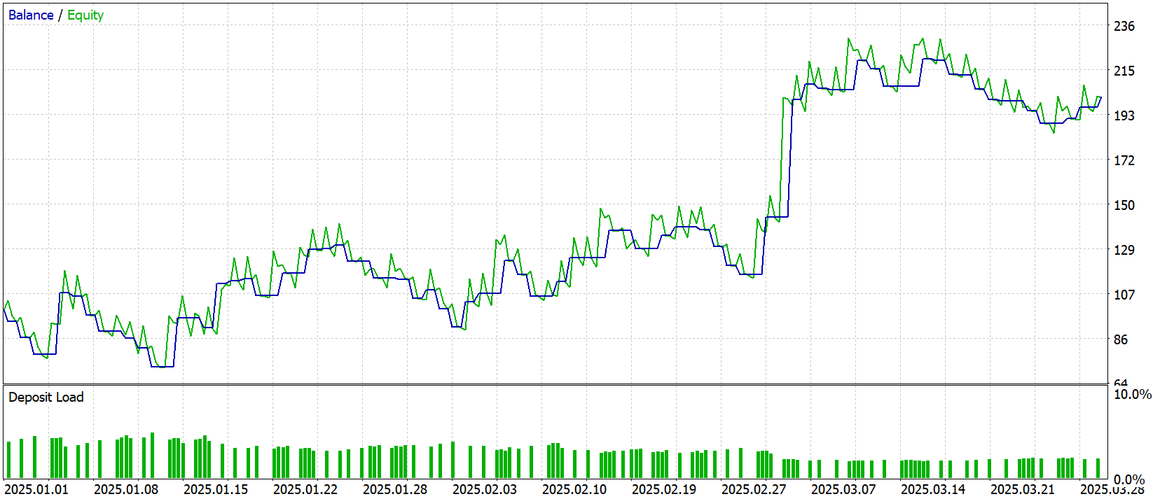
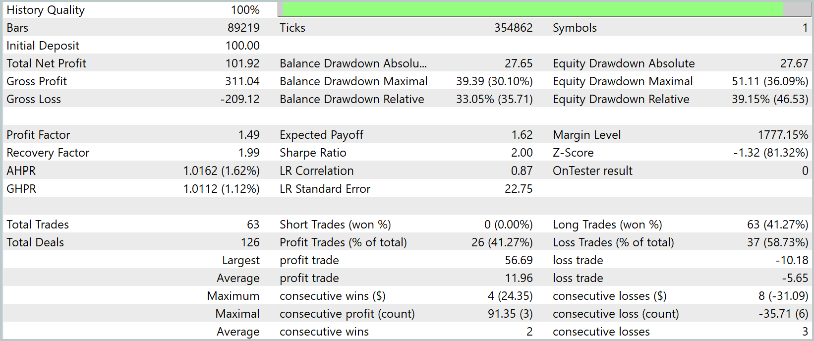
Over three months of testing on the one-minute (M1) chart, our model demonstrated impressive capital growth — from USD 100 to almost USD 202, more than doubling the deposit. At the same time, only about 41% of the trades were profitable, but the average gain of USD 12 far exceeded the average loss of USD 5.6, resulting in a profit factor of 1.49. The equity curve clearly shows sharp rallies after each drawdown, and a Recovery Factor of nearly two confirms a rapid recovery from the maximum drawdown of 36%.

Nevertheless, despite all the positives, one serious bias stands out: the model consistently enters only long positions, riding the broader uptrend. This is particularly evident on the one-minute timeframe: as long as prices are rising, the Agent locks in profits, but at the slightest hint of a reversal it misses the opportunity to profit from a short position.

To make the strategy truly versatile, we still need to work on optimizing it.

Conclusion

In the course of our work, we developed a flexible neural network architecture: from adaptive patching and RoPE to complex modules such as Time‑MoEAttention and Actor–Director–Critic. The system is capable of detecting both short-term impulses and long-term trends, and its triple forecast across different forecast horizons makes it robust to market noise. The next step is to optimize the strategy for two-way trading by adding support for both long and short positions and fine-tuning risk management for both directions. Only after completing a phase of extensive testing and fine-tuning based on real-world data will we be able to develop a truly competitive automated trading system.

References

• LightGTS: A Lightweight General Time Series Forecasting Model
• RoFormer: Enhanced Transformer with Rotary Position Embedding
• Other articles in the series

Programs used in the article

#	Name	Type	Description
1	Study.mq5	Expert Advisor	Expert Advisor for offline model training
2	StudyOnline.mq5	Expert Advisor	Expert Advisor for online model training
3	Test.mq5	Expert Advisor	Expert Advisor for testing the model
4	Trajectory.mqh	Class library	Structure describing the system state and model architecture
5	NeuroNet.mqh	Class library	Class library for building neural networks
6	NeuroNet.cl	Library	Code library for an OpenCL program