

Cricket Algorithm (CA)
 233
233
 0
0

Table of Contents
Introduction
Let us examine another relatively new optimization algorithm. The Cricket Algorithm (CA) is a metaheuristic method developed by Canayaz and Karci in 2015 and published in the journal Applied Intelligence. The algorithm draws inspiration from the behavior of crickets in nature, specifically their ability to communicate through sound and move toward other crickets with the loudest chirping. The algorithm is based on the physical laws governing the propagation of sound in the atmosphere, which gives it a unique connection to the real world.
The algorithm combines elements of three well-known metaheuristics: the Bat Algorithm, Particle Swarm Optimization, and the Firefly Algorithm. The frequency-based mechanism for updating velocity and position was borrowed from the Bat Algorithm; the concept of moving toward the best solution was borrowed from Particle Swarm Optimization; and attraction to “brighter” (in this case, louder) individuals was borrowed from the Firefly Algorithm.
Algorithm Implementation
Crickets are insects known for their distinctive chirping on warm summer days. The sound is produced primarily by males by rubbing their elytra together — a process known as stridulation. Crickets use the sounds they make to attract females for mating, drive unwelcome visitors away from their burrows, and warn their conspecifics of danger. Crickets' auditory organs are located on their front legs, which allows them to pinpoint the direction of a sound source and move toward the cricket with the loudest chirping.
In 1987, American physicist A. Dolbear discovered a correlation between the chirping frequency of crickets and air temperature. According to Dolbear's law, the number of chirps per minute is directly dependent on the ambient temperature: in warm weather, crickets chirp more frequently than in cold weather. This relationship is used in the algorithm to model variations in agent behavior. Since crickets communicate through sound, the algorithm applies the physical laws of acoustics to model the interactions between agents. Consider the main formulas.
The speed of sound in air depends on temperature and is calculated using the following formula:
V = 20.1 × √(273 + C); where V is the speed of sound in meters per second, and C is the air temperature in degrees Celsius. At 20°C, the speed of sound is approximately 343 m/s.
Sound frequency is related to propagation speed and wavelength by the following relationship:
f = V / λ; where f is the frequency in hertz, V is the speed of sound, and λ is the wavelength. In the context of the algorithm, wavelength is interpreted as the distance between the cricket and the best solution in the population.
Sound intensity decreases in inverse proportion to the square of the distance from the source (the inverse-square law):
I = W / (4πr²); where I is the sound intensity in W/m², W is the source power in watts, and r is the distance from the source in meters. Therefore, sound power is expressed as W = I × 4πr².
The sound pressure level at a given distance from the source is calculated using the following formula:
Lp = Lw + 10 × log₁₀[Q / (4πr²)]; where Lp is the sound pressure level in decibels, Lw is the sound power level of the source, Q is the directivity factor (assumed to be 1 for uneven terrain and 2 for flat terrain), and r is the distance from the source.
As sound travels through the atmosphere, it is absorbed by the air. The atmospheric absorption value is calculated in accordance with ISO 9613-1:
A_atm = 7.4 × (f² × r / Ø) × 10⁻⁸; where A_atm is the absorption coefficient, f is the sound frequency in hertz, r is the distance in meters, and Ø is the relative humidity in percent. The actual sound pressure level, taking atmospheric absorption into account, is: Lp' = Lp − A_atm.
These physical formulas are used in the algorithm to calculate the attraction coefficient between agents, which allows for the simulation of realistic attenuation of cricket "audibility" with distance.
The Cricket Algorithm is a population-based optimization method. At each iteration, all agents (crickets) update their positions in the search space, seeking to find the global optimum of the objective function. The algorithm consists of several key steps: generating chirping parameters, updating velocity and position by analogy with the Bat Algorithm, selecting a search strategy based on the sound absorption coefficient, and attraction to louder crickets by analogy with the Firefly Algorithm.
During the initialization phase, a population of "n" agents is created, each of which represents a potential solution to the optimization problem. Agent positions are initialized randomly within the allowed search domain. For each agent, the value of the objective function is calculated, and the best solution in the population is determined.
At each iteration, the following sequence of actions is performed for each cricket. First, a random number of chirps, "N", is generated in the range from 0 to 120. According to Dolbear's law, this number is converted to air temperature. The formula for temperature in degrees Celsius is as follows:
T_C = 10 + (N − 40) / 7. At N = 0, the temperature is approximately 4.3°C; at N = 120, it is about 21.4°C. Thus, a random number of chirps determines the “individual” temperature for each cricket at that iteration.
Next, the speed of sound at the given temperature is calculated:
V_i = 20.1 × √(273 + T_C). The speed of sound varies from approximately 335 to 345 m/s depending on the temperature. Next, the distance "λ" from the current cricket to the best solution in the population is determined. This distance is calculated as the Euclidean norm of the difference in coordinates:
λ = ‖x_i − x*‖; where x_i is the position of the current cricket, and x* is the position of the best solution. In practice, the distance is normalized by dividing it by the diagonal of the search space to obtain a dimensionless value in the range from 0 to 1.
The maximum frequency is calculated based on the speed of sound and the distance:
f_max = V_i / λ. The closer the cricket is to the best solution (the smaller λ is), the higher the frequency, which strengthens the attraction. The farther away the cricket is (the larger λ is), the lower the frequency, which allows it to explore the space more freely.
The individual frequency of each cricket is determined using a formula from the Bat Algorithm:
f_i = f_min + (f_max − f_min) × β; where f_min = 0 and β is a random number in the range [0, 1]. Thus, the frequency f_i takes on a random value between zero and f_max.
After the frequency is calculated, the cricket's velocity and position are updated. Velocity update formula:
v_i^t = v_i^(t−1) + (x* − x_i) × f_i + V_i; where v_i^t is the new velocity, v_i^(t−1) is the velocity at the previous iteration, (x* − x_i) is the direction toward the best solution, f_i is the frequency, and V_i is the speed of sound, which introduces a stochastic impulse. Unlike the original Bat Algorithm, the term V_i is added here, which is a unique feature of the Cricket Algorithm.
The new position is calculated as follows:
x_i^t = x_i^(t−1) + v_i^t. It is important to note that the velocity and position are updated for all crickets at each iteration, regardless of the subsequent strategy selection.
After updating the position, the algorithm selects one of two strategies for the subsequent search. The selection is based on the sound absorption coefficient "γ," which is calculated using the atmospheric absorption formula. A random number r is generated in the range [0, 1], and if r > γ, the phase of attraction toward louder crickets is performed (analogous to the Firefly Algorithm). Otherwise, the cricket performs a random walk near the best solution.
The coefficient "γ" depends on frequency and distance: at high frequencies and over long distances, sound absorption is greater, which increases the likelihood of a random walk. This creates an adaptive balance between global exploration of the search space and local exploitation of the solutions found.
Firefly-like attraction phase. If the random number exceeds the absorption coefficient, the cricket performs a phase of attraction toward louder fellow crickets. To do this, all the other crickets in the population are examined, and for each cricket "j" whose sound is louder (i.e., whose objective function value is better) than that of the current cricket "i," attraction is performed.
First, the distance between the crickets is calculated:
r_ij = ‖x_i − x_j‖. Then, using acoustic formulas, the sound power, sound pressure level, atmospheric absorption, and actual sound pressure level are calculated. The attraction coefficient is determined based on these values:
K = K_0 × exp(−γ × r_ij²); where K_0 is a base coefficient that depends on the actual sound pressure level, and γ is a parameter describing the attenuation of attraction with distance.
The cricket's position is updated using the following formula:
x_i = x_i + K × (x_j − x_i) + α × ε; where the first term represents attraction to the louder cricket “j,” and the second term represents random noise with amplitude “α” and a random vector “ε.” The parameter "α" decreases over time according to the formula α = α_0 × 0.95^t, where t is the iteration number, which ensures the transition from exploration to exploitation.
A key feature of the algorithm is that attraction occurs sequentially toward all the louder crickets in the population, rather than just one. This means that if, in a population of 50 crickets, 30 have a better objective function value, the current cricket will be attracted to all 30, creating averaged movement toward the region of good solutions.
If the random number does not exceed the absorption coefficient, the cricket performs a random walk near the best solution:
x_i = x* + 0.01 × rand(0, 1); where x* is the position of the best solution, and the random number scales the deviation. This strategy provides a local search in the vicinity of the best found solution. During the random walk, the cricket's velocity is reset to zero, allowing it to start over from a new point.
After updating the positions of all crickets, the objective function values are calculated for the new positions. If any cricket finds a solution better than the current global best, the global best is updated. The algorithm continues to run until the specified number of iterations is reached.
The algorithm uses the following parameters: population size "n" (typical value 50), initial noise coefficient α_0 = 0.5, attraction decay coefficient γ = 1.0, relative humidity Ø = 50%, and directivity factor Q = 2. The parameter "α" is reduced at each iteration by multiplying it by 0.95, which ensures a gradual transition from global exploration to local optimization.
When implementing the algorithm in practice, it is necessary to take the scaling of quantities into account. Physical formulas involve dimensional quantities (meters, hertz, decibels), whereas the search space can be on an arbitrary scale. For the algorithm to work correctly, the distances are normalized by dividing them by the diagonal of the search space, the speed of sound is normalized relative to a reference value of 340 m/s, and the frequency is limited to reasonable bounds to prevent numerical instability.
The sound absorption coefficient also needs to be normalized to values in the range [0, 1], which ensures meaningful probabilistic switching between search strategies. Without normalization, the atmospheric absorption formula can yield values many times greater than one, which causes the algorithm to degenerate into a pure random walk.
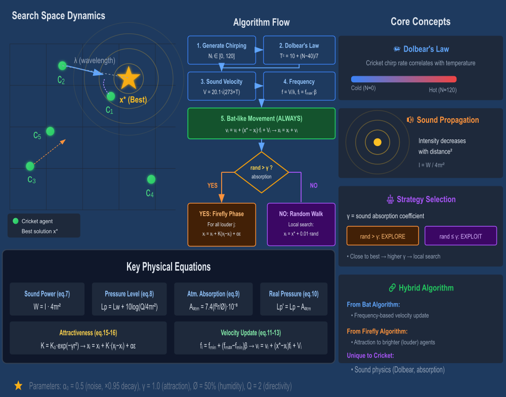
Figure 1. Illustration of the CA-Cricket algorithm in action
The illustration includes Search Space Dynamics (left panel): a visualization of cricket agents in the search space; sound waves emanating from the best solution; movement arrows (velocity, attraction); and the label λ (wavelength/distance to best).
Algorithm Flow (central panel): a step-by-step flowchart of algorithm steps 1–5, including formulas; branching (rand > γ?) YES: Firefly Phase, NO: Random Walk. Key Physical Equations (bottom panel): Eqs. 7–10: acoustic equations; Eqs. 11–13: velocity update; Eqs. 15–16: attraction coefficient. Core Concepts (right panel): Dolbear's law with a temperature scale; Sound Propagation with the inverse square law; Adaptive Strategy Selection; Hybrid Algorithm Nature (Bat + Firefly + unique Cricket features).
Let's write the pseudocode for the CA-Cricket algorithm:
// Initialization
FOR i = 1 TO n DO
xᵢ ← random position within bounds
vᵢ ← 0
fᵢ ← ObjectiveFunction(xᵢ)
END FOR
x* ← position of the agent with the best f
f* ← best value of f
diagonal ← diagonal of the search space
α ← α₀
// Main loop
FOR iter = 1 TO MaxIter DO
α ← α₀ × 0.95^iter
IF α < 0.01 THEN α ← 0.01
FOR i = 1 TO n DO
// Generate chirping parameters
N ← random number from [0, 120]
T ← 10 + (N - 40) / 7
V ← 20.1 × √(273 + T)
// Calculate frequency
λ ← ‖xᵢ - x*‖ / diagonal
f_max ← (V / 340) / λ
fᵢ ← f_max × random number from [0, 1]
// Update velocity and position (always executed)
FOR each coordinate c DO
direction ← (x*[c] - xᵢ[c]) / range[c]
impulse ← (V/340 - 1) × 0.1 × random value from [-1, 1]
vᵢ[c] ← vᵢ[c] + direction × fᵢ × range[c] × 0.1 + impulse × range[c]
vᵢ[c] ← clamp(vᵢ[c], -0.3 × range[c], 0.3 × range[c])
xᵢ[c] ← xᵢ[c] + vᵢ[c]
END FOR
// Strategy selection
γ ← 0.1 + 0.4 × (1 - λ)
r ← random number from [0, 1]
IF r > γ THEN
// Attraction phase (Firefly)
FOR j = 1 TO n DO
IF fⱼ > fᵢ THEN
r_ij ← ‖xᵢ - xⱼ‖ / diagonal
K ← calculate the attraction coefficient using the acoustic formulas
FOR each coordinate c DO
xᵢ[c] ← xᵢ[c] + K × (xⱼ[c] - xᵢ[c]) + α × range[c] × random value from [-0.5, 0.5]
END FOR
END IF
END FOR
ELSE
// Random walk
FOR each coordinate c DO
xᵢ[c] ← x*[c] + α × 0.2 × range[c] × random value from [-1, 1]
vᵢ[c] ← 0
END FOR
END IF
// Coordinate bounds
xᵢ ← clamp to the search bounds
// Update the best solution
fᵢ ← ObjectiveFunction(xᵢ)
IF fᵢ > f* THEN
f* ← fᵢ
x* ← xᵢ
END IF
END FOR
END FOR
RETURN x*, f*
END
Now we can begin implementing the algorithm. The S_CA_Velocity auxiliary structure will be used to store the velocity vector of an individual agent. The structure contains a single field — a dynamic array "v" — whose dimension corresponds to the number of coordinates in the search space. Using a separate structure to store velocities will allow us to organize an array of velocities for all agents in the population and provide convenient access to each agent's velocity components by coordinate index.
//————————————————————————————————————————————————————————————————————
struct S_CA_Velocity
{
    double v [];
};
//————————————————————————————————————————————————————————————————————
The C_AO_CA_Cricket class implements the Cricket Algorithm and inherits from the base class C_AO. The class contains public and private members that provide the algorithm's full functionality.
The public members of the class include two configurable algorithm parameters. The alpha0 parameter specifies the initial value of the noise coefficient used in the formulas for updating agent positions. The gammaFirefly parameter specifies the attenuation coefficient for attraction during the agent interaction phase, by analogy with the Firefly Algorithm. Both parameters can be modified via the "params" array of the base class, which allows the algorithm's behavior to be customized without recompilation.
Private class members store the algorithm's internal state. The "alpha" variable contains the current value of the noise coefficient, which decreases with each iteration. The currentEpoch variable tracks the current iteration number of the algorithm. The "humidity" constant specifies the relative humidity of the air as a percentage and is used in the formula for atmospheric sound absorption. The "Q" constant defines the sound directivity factor, which has a value of 2 for flat terrain. The "vel" array, of type S_CA_Velocity, stores the velocity vectors of all agents in the population. The "pi" constant contains the value of pi for trigonometric calculations. The V_ref variable specifies a reference speed of sound of 340 m/s, relative to which the calculated speeds of sound are normalized. The "maxDiagonal" variable stores the length of the diagonal of the search space and is used to normalize distances between agents.
The SetParams method is designed to apply parameters specified by the user via the "params" array. The method retrieves values from the array and assigns them to the corresponding class variables: popSize receives the integer value of the first element, "alpha0" receives the value of the second element, and gammaFirefly receives the value of the third element. This method must be called after changing the values in the "params" array to update the algorithm's internal variables.
//————————————————————————————————————————————————————————————————————
class C_AO_CA_Cricket : public C_AO
{
  public: //----------------------------------------------------------
  ~C_AO_CA_Cricket () { }

  C_AO_CA_Cricket ()
  {
    ao_name = "CA_Cricket";
    ao_desc = "Cricket Algorithm";
    ao_link = "https://www.mql5.com/en/articles/21058";

    popSize      = 50;
    alpha0       = 0.5;
    gammaFirefly = 1.0;

    ArrayResize (params, 3);
    params [0].name = "popSize";      params [0].val = popSize;
    params [1].name = "alpha0";       params [1].val = alpha0;
    params [2].name = "gammaFirefly"; params [2].val = gammaFirefly;
  }

  void SetParams ()
  {
    popSize      = (int)params [0].val;
    alpha0       = params [1].val;
    gammaFirefly = params [2].val;
  }

  bool Init (const double &rangeMinP  [],
             const double &rangeMaxP  [],
             const double &rangeStepP [],
             const int     epochsP);

  void Moving   ();
  void Revision ();

  //------------------------------------------------------------------
  double alpha0;
  double gammaFirefly;

  private://----------------------------------------------------------
  double alpha;
  int    currentEpoch;
  double humidity;
  double Q;

  S_CA_Velocity vel [];

  double pi;
  double V_ref;         // Reference speed of sound (340 m/s)
  double maxDiagonal;   // Search space diagonal
};
//————————————————————————————————————————————————————————————————————
The Init method performs full initialization of the algorithm before optimization begins. The method takes four parameters: the rangeMinP and rangeMaxP arrays define the boundaries of the search space for each coordinate, the rangeStepP array specifies the discretization step for each coordinate, and the epochsP parameter specifies the maximum number of iterations.
At the beginning of the method, the base class StandardInit method is called, which performs standard initialization of the population and internal data structures. After successful standard initialization, the initial values of the internal variables are set. The current noise coefficient "alpha" is set to "alpha0". The currentEpoch iteration counter is reset to zero. The environmental constants are initialized with fixed values: humidity "humidity" = 50%, directivity factor Q = 2.0, pi = 3.14, and reference speed of sound "V_ref" = 340 m/s.
Next, the diagonal of the search space, maxDiagonal, is calculated. To do this, the squares of the ranges for each coordinate are summed, and then the square root of the sum is calculated. If the calculated diagonal is less than 10⁻¹⁰, it is forcibly set to one to prevent division by zero during subsequent distance normalization.
The final step in the initialization process is to create an array of velocities. The "vel" array is resized to popSize elements. For each agent, a velocity vector of dimension "coords" is created, with all its components initialized to zero. The method returns 'true' upon successful completion of initialization.
//————————————————————————————————————————————————————————————————————
bool C_AO_CA_Cricket::Init (const double &rangeMinP  [],
                            const double &rangeMaxP  [],
                            const double &rangeStepP [],
                            const int     epochsP)
{
  if (!StandardInit (rangeMinP, rangeMaxP, rangeStepP)) return false;

  //------------------------------------------------------------------
  alpha        = alpha0;
  currentEpoch = 0;

  humidity     = 50.0;
  Q            = 2.0;
  pi           = 3.14;
  V_ref        = 340.0;

  // Compute the diagonal of the space for normalization
  maxDiagonal = 0.0;
  for (int c = 0; c < coords; c++)
  {
    double rangeC = rangeMax [c] - rangeMin [c];
    maxDiagonal += rangeC * rangeC;
  }
  maxDiagonal = sqrt (maxDiagonal);
  if (maxDiagonal < 1e-10) maxDiagonal = 1.0;

  ArrayResize (vel, popSize);
  for (int i = 0; i < popSize; i++)
  {
    ArrayResize (vel [i].v, coords);
    for (int c = 0; c < coords; c++)
    {
      vel [i].v [c] = 0.0;
    }
  }

  return true;
}
//————————————————————————————————————————————————————————————————————
The Moving method implements the core logic for moving agents within the search space and is called at each iteration of the algorithm. The method takes no parameters and returns no values; it modifies the positions of the agents directly in the "a" array of the base class.
On the first call to the method, when the "revision" flag is 'false', the initial initialization of the agent positions is performed. For each agent and each coordinate, a random value within the permissible range is generated using the RNDfromCI function, after which the value is mapped to the discretization grid using the SeInDiSp function. The agent's velocity components are set to zero. After all agents have been initialized, the "revision" flag is set to 'true', and the method exits.
On subsequent calls to the method, a full cycle of position updates is performed. At the beginning, the iteration counter currentEpoch is incremented, and the noise coefficient "alpha" is recalculated using the exponential decay formula: "alpha" is multiplied by 0.95 raised to the power of the iteration number. If "alpha" falls below 0.01, the value is fixed at this minimum level to maintain a minimum level of stochasticity in the search.
Next, for each agent in the population, a sequence of calculations is performed according to the algorithm's pseudocode. A random number of chirps, "Ni", is generated in the range from 0 to 120. According to Dolbear's law, the air temperature is calculated in degrees Celsius. The speed of sound "Vi" is calculated based on the temperature.
The distance "lambda_raw" from the current agent to the best solution "cB" is calculated as the Euclidean norm of the coordinate differences. The distance is normalized by dividing it by the search-space diagonal maxDiagonal; the result is constrained to the range from 0.001 to 1.0 to ensure numerical stability.
The speed of sound is normalized by dividing it by the reference value "V_ref," resulting in "Vi_norm" being close to one. The maximum frequency "f_max" is calculated as the ratio of "Vi_norm" to "lambda" and is limited to the range from 0.01 to 10.0. The individual frequency "fi" is defined as the product of "f_max" and a random number "beta" in the range from 0 to 1.
The velocity is updated for each of the agent's coordinates. The normalized direction toward the best solution is calculated as the coordinate difference divided by the range. The impulse "V_impulse" is calculated based on the deviation of "Vi_norm" from one, with a random factor added. The new velocity is the sum of the previous velocity, the product of the direction, frequency, range, and a coefficient of 0.1, and the impulse multiplied by the range. The velocity is limited in absolute value to 0.3 times the coordinate range. The agent's position is updated by adding the velocity vector to its current coordinates.
The absorption coefficient "gammaAbsorption" is calculated using a simplified formula: 0.1 plus 0.4 multiplied by the difference between one and "lambda." Thus, agents that are close to the best solution have a higher coefficient and perform local search more frequently, while agents that are farther away participate more often in global exploration.
A random number is generated, and if it exceeds gammaAbsorption, the attraction phase toward louder crickets is performed. For each other agent "j" with a better objective function value, the normalized distance "r_ij" is calculated. Using acoustic formulas, the sound power "Ps," the sound pressure level "Lp," atmospheric absorption "A_atm," and the actual sound pressure level "R_Lp" are calculated. The attraction coefficient "K_0" is determined using a sigmoid function of R_Lp, and the final coefficient K_i accounts for exponential attenuation with distance. The agent's position is shifted toward agent "j" in proportion to K_i, with random noise added and scaled by the coefficient "alpha." Attraction is applied sequentially to all louder agents without breaking the loop.
If the random number does not exceed gammaAbsorption, the algorithm performs a random walk near the best solution. The new position is calculated as the coordinates of the best solution "cB" plus a random deviation scaled by the product of "alpha," the coefficient 0.2, and the coordinate range. The agent's velocity is reset to zero. At the end of the loop over agents, the coordinates of each agent are clipped to the valid range and snapped to the discretization grid by the SeInDiSp function.
//————————————————————————————————————————————————————————————————————
void C_AO_CA_Cricket::Moving ()
{
  //------------------------------------------------------------------
  if (!revision)
  {
    for (int i = 0; i < popSize; i++)
    {
      for (int c = 0; c < coords; c++)
      {
        a [i].c [c] = u.RNDfromCI (rangeMin [c], rangeMax [c]);
        a [i].c [c] = u.SeInDiSp (a [i].c [c], rangeMin [c], rangeMax [c], rangeStep [c]);
        vel [i].v [c] = 0.0;
      }
    }
    revision = true;
    return;
  }

  //------------------------------------------------------------------
  currentEpoch++;

  alpha = alpha0 *pow (0.95, currentEpoch);
  if (alpha < 0.01) alpha = 0.01;

  //==================================================================
  for (int i = 0; i < popSize; i++)
  {
    //================================================================
    // N_i ∈ [0, 120]
    //================================================================
    double Ni = u.RNDfromCI (0.0, 120.0);

    //================================================================
    // eq. 3: T_C = 10 + (N - 40) / 7
    //================================================================
    double T_C = 10.0 + (Ni - 40.0) / 7.0;

    //================================================================
    // eq. 4: V = 20.1 * sqrt(273 + C)
    //================================================================
    double Vi = 20.1 * MathSqrt (273.0 + T_C);

    //================================================================
    // λ — NORMALIZED distance to the best solution [0, 1]
    //================================================================
    double lambda_raw = 0.0;
    for (int c = 0; c < coords; c++)
    {
      double diff = a [i].c [c] - cB [c];
      lambda_raw += diff * diff;
    }
    lambda_raw = MathSqrt (lambda_raw);

    // Normalization to [0, 1]
    double lambda = lambda_raw / maxDiagonal;
    if (lambda < 0.001) lambda = 0.001;
    if (lambda > 1.0) lambda = 1.0;

    //================================================================
    // eq. 5: f = V / λ
    // Normalize V_i relative to V_ref to obtain f ∈ [0, ~2]
    //================================================================
    double Vi_norm = Vi / V_ref;  // ≈ [0.98, 1.02]
    double f_max = Vi_norm / lambda;  // Now the values are reasonable

    // Limit f_max for stability
    if (f_max > 10.0) f_max = 10.0;
    if (f_max < 0.01) f_max = 0.01;

    //================================================================
    // eq. 11: f_i = f_min + (f_max - f_min) * β
    //================================================================
    double beta  = u.RNDprobab ();
    double f_min = 0.0;
    double fi    = f_min + (f_max - f_min) * beta;

    //================================================================
    // eq. 12: v_i = v_i + (x* - x_i) * f_i + V_i (normalized)
    //================================================================
    for (int c = 0; c < coords; c++)
    {
      double rangeC = rangeMax [c] - rangeMin [c];

      // Normalized direction
      double diff_to_best = (cB [c] - a [i].c [c]) / rangeC;

      // V_i as a normalized impulse
      double V_impulse = (Vi_norm - 1.0) * 0.1 * u.RNDfromCI (-1.0, 1.0);

      // eq. 12: v = v + direction * f + V
      vel [i].v [c] = vel [i].v [c] + diff_to_best * fi * rangeC * 0.1 + V_impulse * rangeC;

      // Velocity limit
      double maxVel = rangeC * 0.3;
      vel [i].v [c] = MathMax (-maxVel, MathMin (maxVel, vel [i].v [c]));
    }

    //================================================================
    // eq. 13: x_i = x_i + v_i
    //================================================================
    for (int c = 0; c < coords; c++)
    {
      a [i].c [c] = a [i].c [c] + vel [i].v [c];
    }

    //================================================================
    // γ — normalized absorption coefficient
    // Use a simplified formula to obtain γ ∈ [0.1, 0.5]
    //================================================================
    // The closer to the best solution (small lambda) → the larger γ → the more local search
    // The farther away (large lambda) → the smaller γ → the more global search
    double gammaAbsorption = 0.1 + 0.4 * (1.0 - lambda);

    //================================================================
    // if rand[0,1] > γ
    //================================================================
    double rnd = u.RNDprobab ();

    if (rnd > gammaAbsorption)
    {
      //--------------------------------------------------------------
      // FIREFLY PHASE: attraction to louder ones
      //--------------------------------------------------------------
      for (int j = 0; j < popSize; j++)
      {
        if (j != i && a [j].f > a [i].f)
        {
          //----------------------------------------------------------
          // r_ij — NORMALIZED distance [0, 1]
          //----------------------------------------------------------
          double r_ij_raw = 0.0;
          for (int c = 0; c < coords; c++)
          {
            double diff = a [i].c [c] - a [j].c [c];
            r_ij_raw += diff * diff;
          }
          r_ij_raw = MathSqrt (r_ij_raw);

          double r_ij = r_ij_raw / maxDiagonal;
          if (r_ij < 0.001) r_ij = 0.001;

          //----------------------------------------------------------
          // eq. 7: Ps = I * 4πr² (normalized)
          //----------------------------------------------------------
          double I_j = 1.0;  // Normalized intensity
          double Ps  = I_j * 4.0 * pi * r_ij * r_ij;

          //----------------------------------------------------------
          // eq. 8: Lp = Lw + 10*log[Q / (4πr²)]
          //----------------------------------------------------------
          double Lw = 10.0 * MathLog10 (Ps + 1e-10);
          double Lp = Lw + 10.0 * MathLog10 (Q / (4.0 * pi * r_ij * r_ij + 1e-10));

          //----------------------------------------------------------
          // eq. 9: A_atm = 7.4 * (f²r / Ø) * 10⁻⁸
          // For normalized values, we scale
          //----------------------------------------------------------
          double A_atm = 7.4 * (fi * fi * r_ij / humidity) * 0.01;

          //----------------------------------------------------------
          // eq. 10: R_Lp = Lp - A_atm
          //----------------------------------------------------------
          double R_Lp = Lp - A_atm;

          //----------------------------------------------------------
          // eq. 15, 16: K = K_0 * exp(-γ * r²)
          //----------------------------------------------------------
          double K_0 = 1.0 / (1.0 + MathExp (-R_Lp / 5.0));
          double K_i = K_0 * MathExp (-gammaFirefly * r_ij * r_ij);

          //----------------------------------------------------------
          // eq. 17: x_i = x_i + K * direction + α * ε
          //----------------------------------------------------------
          for (int c = 0; c < coords; c++)
          {
            double rangeC = rangeMax [c] - rangeMin [c];

            double direction  = a [j].c [c] - a [i].c [c];
            double attraction = K_i * direction;

            double epsilon = u.RNDfromCI (-0.5, 0.5);
            double noise   = alpha * rangeC * epsilon;

            a [i].c [c] = a [i].c [c] + attraction + noise;
          }
          // No break—attraction to all louder crickets
        }
      }
    }
    else
    {
      //--------------------------------------------------------------
      // eq. 14: random walk
      // x_i = x_best + ε * scale
      //
      // The scale depends on alpha (it decreases over time)
      //--------------------------------------------------------------
      for (int c = 0; c < coords; c++)
      {
        double rangeC = rangeMax [c] - rangeMin [c];
        double eps    = u.RNDfromCI (-1.0, 1.0);

        // Adaptive scaling: larger at the beginning, smaller at the end
        double scale = alpha * 0.2;  // 0.1 at the beginning, then decreases

        a [i].c [c] = cB [c] + eps * scale * rangeC;

        vel [i].v [c] = 0.0;
      }
    }

    //================================================================
    // Coordinate clipping and snapping to the step
    //================================================================
    for (int c = 0; c < coords; c++)
    {
      a [i].c [c] = u.SeInDiSp (a [i].c [c], rangeMin [c], rangeMax [c], rangeStep [c]);
    }
  }
}
//————————————————————————————————————————————————————————————————————
The Revision method updates the best solution found based on the results of evaluating the objective function for all agents. The method is called after Moving and after the objective function values for the agents' new positions have been calculated externally.
The method begins by initializing the variables used to find the best agent: "bestIdx" is set to 0, and "bestFit" is set to the value of the first agent's objective function. Next, the loop iterates through all agents, starting with the second one. If the current agent's objective function value exceeds "bestFit," both variables are updated: "bestFit" is set to the new best value, and "bestIdx" is set to the agent's index.
After identifying the best agent in the current population, a comparison is made with the global best solution "fB." If the found value "bestFit" exceeds "fB", the global best is updated. Thus, the "Revision" method ensures that the best solution found is retained throughout the entire optimization process.
//————————————————————————————————————————————————————————————————————
void C_AO_CA_Cricket::Revision ()
{
  int    bestIdx = 0;
  double bestFit = a [0].f;

  for (int i = 1; i < popSize; i++)
  {
    if (a [i].f > bestFit)
    {
      bestFit = a [i].f;
      bestIdx = i;
    }
  }

  if (bestFit > fB)
  {
    fB = bestFit;
    ArrayCopy (cB, a [bestIdx].c, 0, 0, coords);
  }
}
//————————————————————————————————————————————————————————————————————
Test Results
In testing on a standard set of test functions, the algorithm demonstrated relatively modest performance, scoring about 34% of the maximum possible score in the ranking table of optimization algorithms. This metric places the Cricket Algorithm in the lower part of the list of metaheuristics under consideration, indicating that further work is needed to tune and modify it.
=============================
5 Hilly's; Func runs: 10000; result: 0.5836480537501225
25 Hilly's; Func runs: 10000; result: 0.4394651273931123
500 Hilly's; Func runs: 10000; result: 0.3106533980628491
=============================
5 Forest's; Func runs: 10000; result: 0.5352980150573591
25 Forest's; Func runs: 10000; result: 0.3114351845482898
500 Forest's; Func runs: 10000; result: 0.18345680555353047
=============================
5 Megacity's; Func runs: 10000; result: 0.40307692307692317
25 Megacity's; Func runs: 10000; result: 0.19846153846153847
500 Megacity's; Func runs: 10000; result: 0.11247692307692414
=============================
Overall score: 3.07797 (34.20%)
Visualization of the algorithm running on our test functions and an example run on standard test functions.

CA_Cricket on the Hilly test function

CA_Cricket on the Forest test function

CA_Cricket on the Megacity test function

CA_Cricket on the Rastrigin test function

CA_Cricket on the Paraboloid test function
Based on the test results, the CA-Cricket algorithm is shown in the ranking table of the best population-based optimization methods for informational purposes only.
| No. | AO | Description | Hilly | Hilly Final | Forest | Forest Final | Megacity (discrete) | Megacity Final | Final Result | % of MAX | ||||||
| 10 p (5 F) | 50 p (25 F) | 1,000 p (500 F) | 10 p (5 F) | 50 p (25 F) | 1,000 p (500 F) | 10 p (5 F) | 50 p (25 F) | 1,000 p (500 F) | ||||||||
| 1 | DOAdingom | dingo_optimization_algorithm_M | 0.47968 | 0.45367 | 0.46369 | 1.39704 | 0.94145 | 0.87909 | 0.91454 | 2.73508 | 0.78615 | 0.86061 | 0.84805 | 2.49481 | 6.627 | 73.63 |
| 2 | ANS | across-neighborhood search | 0.94948 | 0.84776 | 0.43857 | 2.23581 | 1.00000 | 0.92334 | 0.39988 | 2.32323 | 0.70923 | 0.63477 | 0.23091 | 1.57491 | 6.134 | 68.15 |
| 3 | CLA | code lock algorithm (joo) | 0.95345 | 0.87107 | 0.37590 | 2.20042 | 0.98942 | 0.91709 | 0.31642 | 2.22294 | 0.79692 | 0.69385 | 0.19303 | 1.68380 | 6.107 | 67.86 |
| 4 | AMOm | animal migration optimization M | 0.90358 | 0.84317 | 0.46284 | 2.20959 | 0.99001 | 0.92436 | 0.46598 | 2.38034 | 0.56769 | 0.59132 | 0.23773 | 1.39675 | 5.987 | 66.52 |
| 5 | (P+O)ES | (P+O) evolution strategies | 0.92256 | 0.88101 | 0.40021 | 2.20379 | 0.97750 | 0.87490 | 0.31945 | 2.17185 | 0.67385 | 0.62985 | 0.18634 | 1.49003 | 5.866 | 65.17 |
| 6 | CTA | comet tail algorithm (joo) | 0.95346 | 0.86319 | 0.27770 | 2.09435 | 0.99794 | 0.85740 | 0.33949 | 2.19484 | 0.88769 | 0.56431 | 0.10512 | 1.55712 | 5.846 | 64.96 |
| 7 | TETA | time evolution travel algorithm (joo) | 0.91362 | 0.82349 | 0.31990 | 2.05701 | 0.97096 | 0.89532 | 0.29324 | 2.15952 | 0.73462 | 0.68569 | 0.16021 | 1.58052 | 5.797 | 64.41 |
| 8 | SDSm | stochastic diffusion search M | 0.93066 | 0.85445 | 0.39476 | 2.17988 | 0.99983 | 0.89244 | 0.19619 | 2.08846 | 0.72333 | 0.61100 | 0.10670 | 1.44103 | 5.709 | 63.44 |
| 9 | BOAm | billiards optimization algorithm M | 0.95757 | 0.82599 | 0.25235 | 2.03590 | 1.00000 | 0.90036 | 0.30502 | 2.20538 | 0.73538 | 0.52523 | 0.09563 | 1.35625 | 5.598 | 62.19 |
| 10 | AAm | archery algorithm M | 0.91744 | 0.70876 | 0.42160 | 2.04780 | 0.92527 | 0.75802 | 0.35328 | 2.03657 | 0.67385 | 0.55200 | 0.23738 | 1.46323 | 5.548 | 61.64 |
| 11 | ESG | evolution of social groups (joo) | 0.99906 | 0.79654 | 0.35056 | 2.14616 | 1.00000 | 0.82863 | 0.13102 | 1.95965 | 0.82333 | 0.55300 | 0.04725 | 1.42358 | 5.529 | 61.44 |
| 12 | SIA | simulated isotropic annealing (joo) | 0.95784 | 0.84264 | 0.41465 | 2.21513 | 0.98239 | 0.79586 | 0.20507 | 1.98332 | 0.68667 | 0.49300 | 0.09053 | 1.27020 | 5.469 | 60.76 |
| 13 | EOm | extremal_optimization_M | 0.76166 | 0.77242 | 0.31747 | 1.85155 | 0.99999 | 0.76751 | 0.23527 | 2.00277 | 0.74769 | 0.53969 | 0.14249 | 1.42987 | 5.284 | 58.71 |
| 14 | BBO | biogeography-based optimization | 0.94912 | 0.69456 | 0.35031 | 1.99399 | 0.93820 | 0.67365 | 0.25682 | 1.86867 | 0.74615 | 0.48277 | 0.17369 | 1.40261 | 5.265 | 58.50 |
| 15 | ACS | artificial cooperative search | 0.75547 | 0.74744 | 0.30407 | 1.80698 | 1.00000 | 0.88861 | 0.22413 | 2.11274 | 0.69077 | 0.48185 | 0.13322 | 1.30583 | 5.226 | 58.06 |
| 16 | DA | dialectical algorithm | 0.86183 | 0.70033 | 0.33724 | 1.89940 | 0.98163 | 0.72772 | 0.28718 | 1.99653 | 0.70308 | 0.45292 | 0.16367 | 1.31967 | 5.216 | 57.95 |
| 17 | BHAm | black hole algorithm M | 0.75236 | 0.76675 | 0.34583 | 1.86493 | 0.93593 | 0.80152 | 0.27177 | 2.00923 | 0.65077 | 0.51646 | 0.15472 | 1.32195 | 5.196 | 57.73 |
| 18 | ASO | anarchy society optimization | 0.84872 | 0.74646 | 0.31465 | 1.90983 | 0.96148 | 0.79150 | 0.23803 | 1.99101 | 0.57077 | 0.54062 | 0.16614 | 1.27752 | 5.178 | 57.54 |
| 19 | RFO | royal flush optimization (joo) | 0.83361 | 0.73742 | 0.34629 | 1.91733 | 0.89424 | 0.73824 | 0.24098 | 1.87346 | 0.63154 | 0.50292 | 0.16421 | 1.29867 | 5.089 | 56.55 |
| 20 | AOSm | atomic orbital search M | 0.80232 | 0.70449 | 0.31021 | 1.81702 | 0.85660 | 0.69451 | 0.21996 | 1.77107 | 0.74615 | 0.52862 | 0.14358 | 1.41835 | 5.006 | 55.63 |
| 21 | TSEA | turtle shell evolution algorithm (joo) | 0.96798 | 0.64480 | 0.29672 | 1.90949 | 0.99449 | 0.61981 | 0.22708 | 1.84139 | 0.69077 | 0.42646 | 0.13598 | 1.25322 | 5.004 | 55.60 |
| 22 | BSA | backtracking_search_algorithm | 0.97309 | 0.54534 | 0.29098 | 1.80941 | 0.99999 | 0.58543 | 0.21747 | 1.80289 | 0.84769 | 0.36953 | 0.12978 | 1.34700 | 4.959 | 55.10 |
| 23 | DE | differential evolution | 0.95044 | 0.61674 | 0.30308 | 1.87026 | 0.95317 | 0.78896 | 0.16652 | 1.90865 | 0.78667 | 0.36033 | 0.02953 | 1.17653 | 4.955 | 55.06 |
| 24 | SRA | successful restaurateur algorithm (joo) | 0.96883 | 0.63455 | 0.29217 | 1.89555 | 0.94637 | 0.55506 | 0.19124 | 1.69267 | 0.74923 | 0.44031 | 0.12526 | 1.31480 | 4.903 | 54.48 |
| 25 | BO | bonobo_optimizer | 0.77565 | 0.63805 | 0.32908 | 1.74278 | 0.88088 | 0.76344 | 0.25573 | 1.90005 | 0.61077 | 0.49846 | 0.14246 | 1.25169 | 4.895 | 54.38 |
| 26 | CRO | chemical reaction optimization | 0.94629 | 0.66112 | 0.29853 | 1.90593 | 0.87906 | 0.58422 | 0.21146 | 1.67473 | 0.75846 | 0.42646 | 0.12686 | 1.31178 | 4.892 | 54.36 |
| 27 | BIO | blood inheritance optimization (joo) | 0.81568 | 0.65336 | 0.30877 | 1.77781 | 0.89937 | 0.65319 | 0.21760 | 1.77016 | 0.67846 | 0.47631 | 0.13902 | 1.29378 | 4.842 | 53.80 |
| 28 | DOA | dream_optimization_algorithm | 0.85556 | 0.70085 | 0.37280 | 1.92921 | 0.73421 | 0.48905 | 0.24147 | 1.46473 | 0.77231 | 0.47354 | 0.18561 | 1.43146 | 4.825 | 53.62 |
| 29 | BSA | bird swarm algorithm | 0.89306 | 0.64900 | 0.26250 | 1.80455 | 0.92420 | 0.71121 | 0.24939 | 1.88479 | 0.69385 | 0.32615 | 0.10012 | 1.12012 | 4.809 | 53.44 |
| 30 | DEA | dolphin_echolocation_algorithm | 0.75995 | 0.67572 | 0.34171 | 1.77738 | 0.89582 | 0.64223 | 0.23941 | 1.77746 | 0.61538 | 0.44031 | 0.15115 | 1.20684 | 4.762 | 52.91 |
| 31 | HS | harmony search | 0.86509 | 0.68782 | 0.32527 | 1.87818 | 0.99999 | 0.68002 | 0.09590 | 1.77592 | 0.62000 | 0.42267 | 0.05458 | 1.09725 | 4.751 | 52.79 |
| 32 | SSG | saplings sowing and growing | 0.77839 | 0.64925 | 0.39543 | 1.82308 | 0.85973 | 0.62467 | 0.17429 | 1.65869 | 0.64667 | 0.44133 | 0.10598 | 1.19398 | 4.676 | 51.95 |
| 33 | BCOm | bacterial chemotaxis optimization M | 0.75953 | 0.62268 | 0.31483 | 1.69704 | 0.89378 | 0.61339 | 0.22542 | 1.73259 | 0.65385 | 0.42092 | 0.14435 | 1.21912 | 4.649 | 51.65 |
| 34 | ABO | african buffalo optimization | 0.83337 | 0.62247 | 0.29964 | 1.75548 | 0.92170 | 0.58618 | 0.19723 | 1.70511 | 0.61000 | 0.43154 | 0.13225 | 1.17378 | 4.634 | 51.49 |
| 35 | (PO)ES | (PO) evolution strategies | 0.79025 | 0.62647 | 0.42935 | 1.84606 | 0.87616 | 0.60943 | 0.19591 | 1.68151 | 0.59000 | 0.37933 | 0.11322 | 1.08255 | 4.610 | 51.22 |
| 36 | FBA | fractal-based algorithm | 0.79000 | 0.65134 | 0.28965 | 1.73099 | 0.87158 | 0.56823 | 0.18877 | 1.62858 | 0.61077 | 0.46062 | 0.12398 | 1.19537 | 4.555 | 50.61 |
| 37 | TSm | tabu search M | 0.87795 | 0.61431 | 0.29104 | 1.78330 | 0.92885 | 0.51844 | 0.19054 | 1.63783 | 0.61077 | 0.38215 | 0.12157 | 1.11449 | 4.536 | 50.40 |
| 38 | BSO | brain storm optimization | 0.93736 | 0.57616 | 0.29688 | 1.81041 | 0.93131 | 0.55866 | 0.23537 | 1.72534 | 0.55231 | 0.29077 | 0.11914 | 0.96222 | 4.498 | 49.98 |
| 39 | WOAm | whale optimization algorithm M | 0.84521 | 0.56298 | 0.26263 | 1.67081 | 0.93100 | 0.52278 | 0.16365 | 1.61743 | 0.66308 | 0.41138 | 0.11357 | 1.18803 | 4.476 | 49.74 |
| 40 | AEFA | artificial electric field algorithm | 0.87700 | 0.61753 | 0.25235 | 1.74688 | 0.92729 | 0.72698 | 0.18064 | 1.83490 | 0.66615 | 0.11631 | 0.09508 | 0.87754 | 4.459 | 49.55 |
| 41 | AEO | artificial ecosystem-based optimization algorithm | 0.91380 | 0.46713 | 0.26470 | 1.64563 | 0.90223 | 0.43705 | 0.21400 | 1.55327 | 0.66154 | 0.30800 | 0.28563 | 1.25517 | 4.454 | 49.49 |
| 42 | CAm | camel algorithm M | 0.78684 | 0.56042 | 0.35133 | 1.69859 | 0.82772 | 0.56041 | 0.24336 | 1.63149 | 0.64846 | 0.33092 | 0.13418 | 1.11356 | 4.444 | 49.37 |
| 43 | ACOm | ant colony optimization M | 0.88190 | 0.66127 | 0.30377 | 1.84693 | 0.85873 | 0.58680 | 0.15051 | 1.59604 | 0.59667 | 0.37333 | 0.02472 | 0.99472 | 4.438 | 49.31 |
| 44 | CMAES | covariance_matrix_adaptation_evolution_strategy | 0.76258 | 0.72089 | 0.00000 | 1.48347 | 0.82056 | 0.79616 | 0.00000 | 1.61672 | 0.75846 | 0.49077 | 0.00000 | 1.24923 | 4.349 | 48.33 |
| 45 | DA_duelist | duelist_algorithm | 0.92782 | 0.53778 | 0.27792 | 1.74352 | 0.86957 | 0.47536 | 0.18193 | 1.52686 | 0.62153 | 0.33569 | 0.11715 | 1.07437 | 4.345 | 48.28 |
| CA_Cricket | cricket_algorithm | 0.58364 | 0.43946 | 0.31065 | 1.33375 | 0.53529 | 0.31143 | 0.18346 | 1.03018 | 0.40307 | 0.19846 | 0.11247 | 0.71400 | 3.078 | 34.20 | |
| RW | random walk | 0.48754 | 0.32159 | 0.25781 | 1.06694 | 0.37554 | 0.21944 | 0.15877 | 0.75375 | 0.27969 | 0.14917 | 0.09847 | 0.52734 | 2.348 | 26.09 | |
Conclusions
By observing how the algorithm behaves, one can note its distinctive approach to exploring the search space. The combination of a Bat Algorithm-like velocity update mechanism with Firefly Algorithm-like attraction creates an interesting pattern of population movement, in which agents simultaneously move toward the global best solution and are drawn toward their locally best neighbors. The physical formulas governing sound propagation add an additional level of complexity to these interactions, although their impact on overall performance requires more detailed study.
The results indicate that the Cricket Algorithm, in its current implementation, requires further tuning to achieve competitive performance. Potential areas for improvement include adjusting the coefficients in the velocity and position update formulas, modifying the mechanism for calculating the absorption coefficient to achieve a more balanced switch between global exploration and local exploitation, and possibly revising the logic of attraction to multiple sources. A promising avenue is to study the impact of individual components of the algorithm on its performance in order to identify the most significant factors and determine their optimal settings.
Despite current performance limitations, the Cricket Algorithm is of interest as an example of how the physical laws of acoustics can be integrated into a metaheuristic optimization method. The unique combination of Dolbear's law, sound propagation and absorption formulas, and classical swarm intelligence mechanisms creates a conceptually rich algorithm, whose potential can be realized through proper calibration of parameters and possible modification of individual formulas. Future research could focus on identifying optimal parameter values for various classes of problems, as well as on developing adaptive tuning mechanisms that take into account the characteristics of a specific optimization problem.
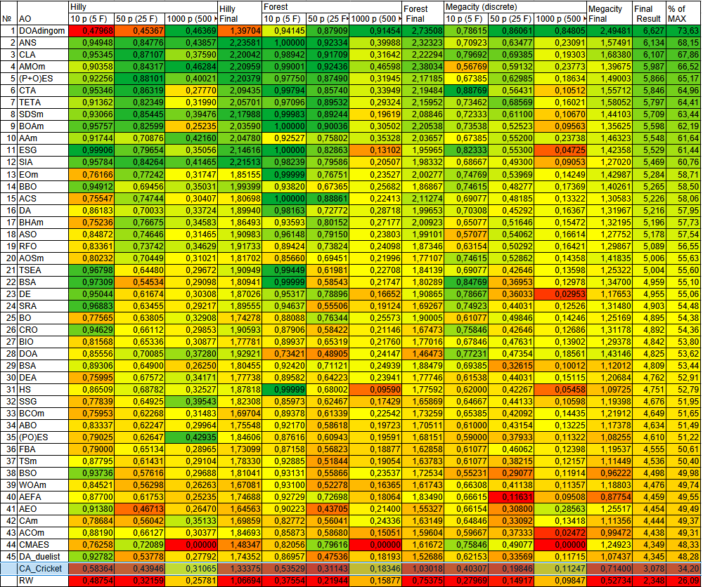
Figure 2. Color gradation of algorithms by the corresponding tests
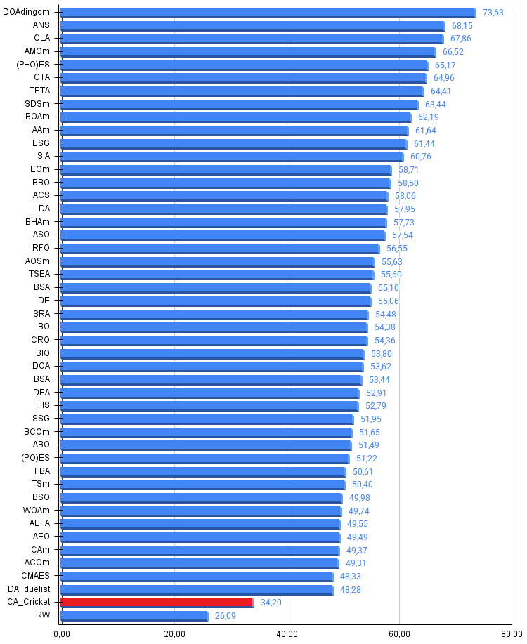
Figure 3. Histogram of algorithm test results (on a scale from 0 to 100; the higher the score, the better, where 100 is the maximum possible theoretical result; the archive contains a script for calculating the ranking table)
Pros and cons of the CA_Cricket algorithm:
Pros:
- It performs best on medium- and high-dimensional functions.
Cons:
- It does not handle low-dimensional functions well enough.
An archive containing the current versions of the algorithm code is attached to the article. The author of this article does not guarantee absolute accuracy in the descriptions of the canonical algorithms; many of them have been modified to improve their search capabilities. The conclusions and judgments presented in the articles are based on the results of the experiments conducted.
Software used in this article
| # | Name | Type | Description |
|---|---|---|---|
| 1 | #C_AO.mqh | Include file | Parent class for population-based optimization algorithms |
| 2 | #C_AO_enum.mqh | Include file | Enumeration of population-based optimization algorithms |
| 3 | TestFunctions.mqh | Include file | Test function library |
| 4 | TestStandFunctions.mqh | Include file | Test bench function library |
| 5 | Utilities.mqh | Include file | Utility function library |
| 6 | CalculationTestResults.mqh | Include file | Script for calculating results for the comparison table |
| 7 | Testing AOs.mq5 | Script | Unified test bench for all population-based optimization algorithms |
| 8 | Simple use of population optimization algorithms.mq5 | Script | A simple example of using population-based optimization algorithms without visualization |
| 9 | Test_AO_CA_Cricket.mq5 | Script | Test bench for CA_Cricket |
Translated from Russian by MetaQuotes Ltd.
Original article: https://www.mql5.com/ru/articles/21058
Warning: All rights to these materials are reserved by MetaQuotes Ltd. Copying or reprinting of these materials in whole or in part is prohibited.
This article was written by a user of the site and reflects their personal views. MetaQuotes Ltd is not responsible for the accuracy of the information presented, nor for any consequences resulting from the use of the solutions, strategies or recommendations described.

 Features of Custom Indicators Creation
 A Forgotten Classic in Volume Analysis: The Finite Volume Elements Indicator for Today's Markets
 Features of Experts Advisors
 Neural Networks in Trading: Decomposition Instead of Scaling — Building Modules

- Free trading apps
- Over 8,000 signals for copying
- Economic news for exploring financial markets
You agree to website policy and terms of use