Low-Frequency Quantitative Strategies in MetaTrader 5 (Part 5): Pre-Backtest Evaluation of Machine-Learning-Generated Signals Through Formulaic Alphas

“One day in the near future, machine learning will dominate finance, science will curtail guessing, and investing will not mean gambling. I would like the reader to play a part in that revolution.” (Marcos López de Prado, Advances in Financial Machine Learning)

Introduction

Machine learning became part of retail traders' toolkits. However, after several years of widespread automated signal mining, a cost became evident in the early 2010s: techniques that once produced real edges began generating an increasing number of low-value signals. With many machines working 24/7 on the same data universe, the number of signals surged; most of them were weak or short-lived. 

In 2016, in an effort to address these problems, Dr. Zura Kakushadze proposed a method to formalize predictive signals using an algebraic expression. He called them formulaic alphas. These algebraic expressions should facilitate combining dozens or hundreds of weak signals into a single “mega-signal” and make these machine-generated signals explainable and auditable.

This article explains how formulaic alphas are built and how they can be used to evaluate machine-generated trading signals without embedding them in a full trading strategy or running backtests.

The question of many weak or ephemeral machine-generated alphas

We started this series with two proven old-school strategies: a volatility-adjusted momentum-based intraday system that leverages the opening range breakouts and a regime-adaptive swing trading system that uses relative price to identify trend exhaustion in bullish markets and mean-reverting pullbacks in bear markets.

The first is an ancient trading strategy that remains effective nowadays, not only in our backtests but also in extensive research conducted by the Swiss Institute for Finance around 2023. The second was developed and published around 2010 by a quantitative systems designer in partnership with an institutional portfolio manager. Both trading systems were developed based on human creativity, market knowledge, econometrics, and possibly trial and error. None of them is obsolete. Both are functional trading systems today, as they were when they were developed. Among other features, like sound risk management, their signals are backed by a solid economic rationale.

However, a solid economic rationale is a feature we cannot take for granted in machine-learning-generated signals.

“An automated search is subject to three problems resulting from its large scale: computational load, the inability to manually inspect every component, and lower confidence in each alpha. An automated search usually involves combining different data with different functions by trial and error. As a result, a high level of computational power is usually needed. Optimizations that reduce memory usage and improve speed can result in finding more and better alphas. The large number of combinations also means that it is impossible to inspect each of the resulting formulas by hand. Even if one wants to investigate a sample manually, the alpha expression can be very complicated and without obvious financial significance. Moreover, the sheer number of trials means that it is common for combinations that make no mathematical and economic sense to be erroneously recognized as alphas through survival bias.” [2]

The term “alpha” is well-known in finance. But here, in the context of formulaic alphas research, it requires some clarification. 

The standard meaning of the term “alpha” in finance is a measure of investment performance, describing returns that exceed a benchmark index, the S&P 500, for example.

But for the principal researchers involved in the proposition and development of formulaic alphas, the term has a slightly different meaning.

"[...] we use the term a little differently. We design and develop “alphas”, individual trading signals that seek to add value to a portfolio. [...] Fundamentally, an alpha is an idea about how the market works. There are an infinite number of ideas, hypotheses, or rules that can be extrapolated, and the number of possibilities is constantly growing with the rapid increase in new data and market knowledge. Each of these ideas could be an alpha, but many are not. An alpha is an automated predictive model that describes, or decodes, some market relations. We design alphas as algorithms, a combination of mathematical expressions, computer source code, and configuration parameters. An alpha contains rules for converting input data to positions or trades to be executed in the financial securities markets." (emphasis is ours) [2]

With terminology clarified, we return to the main problem: how to manage, make transparent, and monetize many potentially weak machine-learning-generated alphas.

In February 2016, Dr. Zura Kakushadze published a paper entitled “How To Combine a Billion Alphas” containing “an explicit algorithm and source code for computing optimal weights for combining a large number N of alphas.” [3]

A month later, he published “101 Formulaic Alphas”, which is among the top-ten downloads on quantitative trading at SSRN at the time of writing.

“[...] the 101 alphas we present here are not 'toy' alphas but real-life trading alphas used in production. In fact, 80 of these alphas are in production as of this writing. To our knowledge, this is the first time such a large number of real-life explicit formulaic alphas appear in the literature. This should come as no surprise: naturally, quant trading is highly proprietary and secretive. Our goal here is to provide a glimpse into the complex world of modern and ever-evolving quantitative trading and help demystify it to any degree possible.” [4]

Thus, we are talking about how to combine such a large number of trading signals that they can, at least theoretically, amount to a billion signals. Formulaic alphas were proposed and are being used to address this problem.

Formulaic alphas

Roughly speaking, an alpha is a weighted trading signal, and a formulaic alpha is its algebraic expression.

Let’s take a look at the simplest alpha among the 101 published in Dr. Zura Kakushadze’s paper “101 Formulaic Alphas”, the Alpha #101.

Fig. 1 - Alpha #101 formula

Where:

• (close - open) calculates the intraday price change 
• (high - low) calculates the total intraday price range
• + .001 is only a small constant added to the denominator to prevent division by zero.

This is a momentum alpha. If the stock runs up intraday (close > open), the formula produces a positive signal, suggesting a long position for the next day. If the stock falls intraday (close < open), the formula produces a negative signal, suggesting a short position for the next day. For each day, it gives different values for different stocks. The higher the value, the more likely that the stock will have relatively larger returns in the following days.

It can be represented as a binary expression tree.

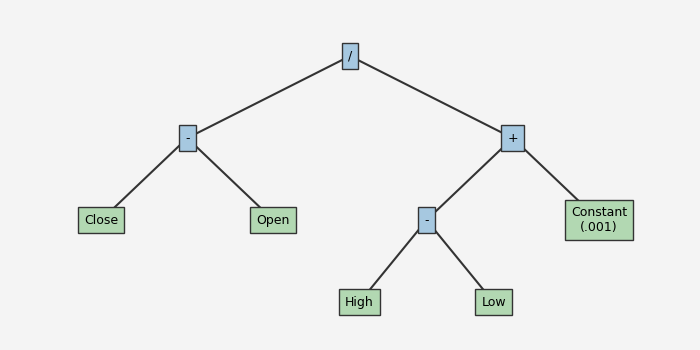
Fig. 2 - Alpha #101 Binary expression tree

The Alpha #101 used as an example above is very simple. Formulaic alphas can carry more information, as shown on the list of functions below.

Components of a formulaic alpha

A formulaic alpha is composed of:

• Functions
• Operators
• Input Data

Once the functions and operators are defined, formulaic alphas are also functional code.

Functions and operators

These are the functions defined in the original paper. Note that the only limitation for this list is that it must be supported by the expression engine parser. It can be extended, shortened, or adapted according to specific needs. We are reproducing the functions and their definitions verbatim.

Below, “{ }” stands for a placeholder. All expressions are case-insensitive.

Function/Operator	Semantics
abs(x), log(x), sign(x), +, -, *, /, >, <, ==, ||, x ? y : z	standard definitions
rank(x)	cross-sectional rank
delay(x, d)	value of x d days ago
correlation(x, y, d)	time-serial correlation of x and y for the past d days
covariance(x, y, d)	time-serial covariance of x and y for the past d days
scale(x, a)	rescaled x such that sum(abs(x)) = a (the default is a = 1)
delta(x, d)	today’s value of x minus the value of x d days ago
signedpower(x, a)	x^a
decay_linear(x, d)	weighted moving average over the past d days with linearly decaying weights d, d – 1, ..., 1 (rescaled to sum up to 1)
indneutralize(x, g)	x cross-sectionally neutralized against groups g (subindustries, industries, sectors, etc.), i.e., x is cross-sectionally demeaned within each group g
ts_{O}(x, d)	operator O applied across the time series for the past d days; a non-integer number of days d is converted to floor(d)
ts_min(x, d)	time series min over the past d days
ts_max(x, d)	time series max over the past d days
ts_argmax(x, d)	which day ts_max(x, d) occurred on
ts_argmin(x, d)	which day ts_min(x, d) occurred on
ts_rank(x, d)	time series rank in the past d days
min(x, d)	ts_min(x, d)
max(x, d)	ts_max(x, d)
sum(x, d)	time series sum over the past d days
product(x, d)	time series product over the past d days
stddev(x, d)	moving time series standard deviation over the past d days

Input Data

Function	Semantics
returns	daily close-to-close returns
open, close, high, low, volume	standard definitions for daily price and volume data
vwap	daily volume-weighted average price
cap	market cap adv{d} = average daily dollar volume for the past d days
IndClass	a generic placeholder for a binary industry classification such as GICS, BICS, NAICS, SIC, etc., in indneutralize(x, IndClass.level), where level = sector, industry, subindustry, etc. Multiple IndClass in the same alpha need not correspond to the same industry classification.

As noted above, these are the functions, operators, and input data described in the original paper. They may be a starting point for a library or an expression engine development.

Having the functions and operators defined, a formulaic alpha is functional code. Given proper input data (the closing price time series in the sample MQL5 implementation below), it should return the score for the respective symbol.

Sample implementation of Alpha #1 in MQL5

Unsurprisingly, the 101 alphas can be classified into three groups, according to the predominant source of analysis:

• Momentum
• Mean-reversion
• Fundamental

Many of them are hybrids that combine, for example, momentum and mean-reversion or fundamental and momentum as the main source of analysis. We say that there are no surprises here because formulaic alphas are, at the end of the day, algebraic descriptions of a potential trading edge over the market, like any other trading strategy.

The Alpha #1, the first listed on the paper, is a momentum one. It explores the volatility asymmetry in equity markets. This is the same principle explored by the MR Swing system we saw in Part 3 of this series. When a stock price is falling, volatility tends to be higher than when the price is rising because institutional traders will usually be hedging or even liquidating positions. In other words, bear markets tend to cause larger smart-money reallocations and move prices faster.

This is the Alpha #1 formula.

Fig. 3 - Alpha #1 formula

And this is the Alpha #1 binary expression tree.

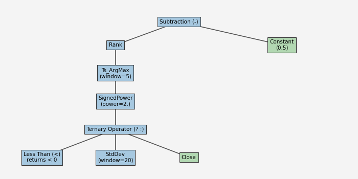
Fig. 4 - Alpha #1 binary expression tree

Let’s start understanding each logical piece of the formula.

Fig. 5 - Alpha #1 ternary operator that performs a conditional logic check

If the daily close-to-close return is negative, we calculate the daily returns standard deviation for the last 20 days. Otherwise, we use the current closing price.

Fig. 6 - Alpha #1 signed power operator

We square the value to amplify the risk spike exponentially and emphasize peaks relative to normal fluctuations.

Fig. 7 - Alpha #1 time series operator returns the specific day in a 5-day lookback window

This time series operator returns the day when the risk reached its peak. We can expect an exhaustion of institutional selling pressure right after this day. 

Fig. 8 - Alpha #1 cross-sectional rank operator ranks the active trading portfolio

The cross-sectional ranking operator sorts the stocks under analysis, mapping their relative values onto a normalized scale from 0.0 to 1.0. 

Fig. 9 - Alpha #1 demeaning transformation

Finally, we have a demeaning transformation. It subtracts the mean from each data point. The result is that it centers the portfolio signal around zero, that is, a dollar-neutral signal between -0.5 and +0.5.

Sample MQL5 Implementation

To make code reuse easy for future implementations of other alphas, we have split the code into the six files you will find attached to this article.

The functions used in Alpha #1 are grouped in the AlphaOperators.mqh header. We leverage the ALGLIB from the MQL5 standard library whenever possible.

//+------------------------------------------------------------------+
//|                                               AlphaOperators.mqh |
//|                             Copyright 2000-2026, MetaQuotes Ltd. |
//|                                                     www.mql5.com |
//+------------------------------------------------------------------+
#property copyright "Copyright 2000-2026, MetaQuotes Ltd."
#property link      "https://www.mql5.com"
#property version   "1.00"

#include <Math\Alglib\alglib.mqh>

//+------------------------------------------------------------------+
//| Time series operators for Alpha #1                                |
//+------------------------------------------------------------------+
class CAlphaOperators
  {
public:
   // Standard Deviation using Alglib
   static double StdDev(const double &data[], int period)
     {
      int size = ArraySize(data);
      if(size < period || period <= 1) return 0;
      
      double buffer[];
      ArrayResize(buffer, period);
      for(int i = 0; i < period; i++)
         buffer[i] = data[size - period + i];
         
      double mean, variance, skewness, kurtosis;
      CBaseStat::SampleMoments(buffer, period, mean, variance, skewness, kurtosis);
      return MathSqrt(variance);
     }

   // SignedPower(x, a) = sign(x) * (|x|^a)
   static double SignedPower(double x, double a)
     {
      if(x == 0.0) return 0.0;
      return (x > 0.0 ? 1.0 : -1.0) * MathPow(MathAbs(x), a);
     }

   // Ts_ArgMax(x, d) - relative index of max value in last d days
   // 1 is today, d is d days ago
   // Paper says: "which day ts_max(x, d) occurred on"
   // Usually in these alphas, 1 is the most recent, d is the oldest in the window.
   static int Ts_ArgMax(const double &data[], int d)
     {
      int size = ArraySize(data);
      if(size < d) return 0;
      
      int max_idx = size - 1;
      double max_val = data[max_idx];
      
      for(int i = 1; i < d; i++)
        {
         int current_idx = size - 1 - i;
         if(data[current_idx] > max_val)
           {
            max_val = data[current_idx];
            max_idx = current_idx;
           }
        }
      // Return 1-based index from the end (1 = today)
      return (size - max_idx);
     }
     
   // Returns: daily close-to-close returns
   static double GetReturns(const string symbol, int index)
     {
      double close0 = iClose(symbol, PERIOD_D1, index);
      double close1 = iClose(symbol, PERIOD_D1, index + 1);
      if(close1 == 0) return 0;
      return (close0 - close1) / close1;
     }
  };
//+------------------------------------------------------------------+

The “rank” function is in the CrossSectional.mqh header for clarity.

//+------------------------------------------------------------------+
//|                                             CrossSectional.mqh |
//|                             Copyright 2000-2026, MetaQuotes Ltd. |
//|                                                     www.mql5.com |
//+------------------------------------------------------------------+
#property copyright "Copyright 2000-2026, MetaQuotes Ltd."
#property link      "https://www.mql5.com"
#property version   "1.00"

#include "UniverseManager.mqh"

//+------------------------------------------------------------------+
//| Cross-sectional operations for 101 Alphas                        |
//+------------------------------------------------------------------+
class CCrossSectional
  {
public:
   // Rank values from 0 to 1
   static void Rank(double &values[])
     {
      int size = ArraySize(values);
      if(size <= 1) return;
      
      int indices[];
      ArrayResize(indices, size);
      for(int i = 0; i < size; i++) indices[i] = i;
      
      // Sort indices based on values
      // We can use a simple sort or a more efficient one if needed
      for(int i = 0; i < size - 1; i++)
        {
         for(int j = i + 1; j < size; j++)
           {
            if(values[indices[i]] > values[indices[j]])
              {
               int temp = indices[i];
               indices[i] = indices[j];
               indices[j] = temp;
              }
           }
        }
        
      double ranked[];
      ArrayResize(ranked, size);
      for(int i = 0; i < size; i++)
        {
         // i is the rank (0 to size-1)
         // Scale to [0, 1]
         ranked[indices[i]] = (double)i / (size - 1);
        }
       
      ArrayCopy(values, ranked);
     }
  };
//+------------------------------------------------------------------+

The symbols selected in the Market Watch, that is, our “portfolio” or universe in alpha lingo, are managed by the CUniverseManager class in the UniverseManager.mqh header.

//+------------------------------------------------------------------+
//|                                              UniverseManager.mqh |
//|                             Copyright 2000-2026, MetaQuotes Ltd. |
//|                                                     www.mql5.com |
//+------------------------------------------------------------------+
#property copyright "Copyright 2000-2026, MetaQuotes Ltd."
#property link      "https://www.mql5.com"
#property version   "1.00"

//+------------------------------------------------------------------+
//| Manages symbols in Market Watch for cross-sectional operations   |
//+------------------------------------------------------------------+
class CUniverseManager
  {
private:
   string            m_symbols[];

public:
                     CUniverseManager(void) { Refresh(); }
                    ~CUniverseManager(void) {}

   // Refresh the list of symbols from Market Watch
   void              Refresh(void)
     {
      int total = SymbolsTotal(true);
      ArrayResize(m_symbols, total);
      for(int i = 0; i < total; i++)
        {
         m_symbols[i] = SymbolName(i, true);
        }
     }

   // Get the number of symbols
   int               GetCount(void) const { return ArraySize(m_symbols); }

   // Get symbol by index
   string            GetSymbol(int index) const
     {
      if(index < 0 || index >= ArraySize(m_symbols)) return "";
      return m_symbols[index];
     }

   // Check if a symbol exists in the universe
   bool              HasSymbol(const string symbol) const
     {
      for(int i=0; i<ArraySize(m_symbols); i++)
         if(m_symbols[i] == symbol) return true;
      return false;
     }
  };
//+------------------------------------------------------------------+

We have a generic base class, CBaseAlpha with only two virtual methods applicable to any alpha. It will be used again when implementing other alphas, including new alphas not included in Dr. Zura Kakushadze’s paper. This base class runs calculations that apply to any alpha. It only has to know about the CUniverseManager class, which is included.

//+------------------------------------------------------------------+
//|                                                    BaseAlpha.mqh |
//|                             Copyright 2000-2026, MetaQuotes Ltd. |
//|                                                     www.mql5.com |
//+------------------------------------------------------------------+
#property copyright "Copyright 2000-2026, MetaQuotes Ltd."
#property link      "https://www.mql5.com"
#property version   "1.00"

#include "UniverseManager.mqh"

//+------------------------------------------------------------------+
//| Base class for any alpha                                         |
//+------------------------------------------------------------------+
class CBaseAlpha
  {
protected:
   CUniverseManager *m_universe;

public:
                     CBaseAlpha(CUniverseManager *universe) : m_universe(universe) {}
   virtual          ~CBaseAlpha(void) {}

   // Pre-calculation for a specific time (useful for cross-sectional alphas)
   virtual void      PreCalculate(const datetime time) {}

   // Main calculation entry point
   // Returns the alpha value for a specific symbol at a specific time
   virtual double    Calculate(const string symbol, const datetime time) = 0;
  };
//+------------------------------------------------------------------+

The calculations that are specific to Alpha #1 are grouped in the Alpha1.mqh header. It includes the above headers for alpha operators/functions and cross-sectional ranking.

//+------------------------------------------------------------------+
//|                                                       Alpha1.mqh |
//|                             Copyright 2000-2026, MetaQuotes Ltd. |
//|                                                     www.mql5.com |
//+------------------------------------------------------------------+
#property copyright "Copyright 2000-2026, MetaQuotes Ltd."
#property link      "https://www.mql5.com"
#property version   "1.00"

#include "..\Include\BaseAlpha.mqh"
#include "..\Include\AlphaOperators.mqh"
#include "..\Include\CrossSectional.mqh"

//+------------------------------------------------------------------+
//| Alpha #1: (rank(Ts_ArgMax(SignedPower(((returns < 0) ?           |
//|          stddev(returns, 20) : close), 2.), 5)) - 0.5)           |
//+------------------------------------------------------------------+
class CAlpha1 : public CBaseAlpha
  {
private:
   double            m_cached_results[];
   datetime          m_last_calc_time;

public:
                     CAlpha1(CUniverseManager *universe) : CBaseAlpha(universe), m_last_calc_time(0) {}

   virtual void      PreCalculate(const datetime time)
     {
      if(m_last_calc_time == time)
         return;
      int count = m_universe.GetCount();
      ArrayResize(m_cached_results, count);
      double raw_values[];
      ArrayResize(raw_values, count);
      for(int i = 0; i < count; i++)
        {
         string symbol = m_universe.GetSymbol(i);
         raw_values[i] = CalculateRawValue(symbol, time);
        }
      // Apply rank
      CCrossSectional::Rank(raw_values);
      for(int i = 0; i < count; i++)
        {
         m_cached_results[i] = raw_values[i] - 0.5;
        }
      m_last_calc_time = time;
     }

   virtual double    Calculate(const string symbol, const datetime time)
     {
      PreCalculate(time);
      for(int i = 0; i < m_universe.GetCount(); i++)
        {
         if(m_universe.GetSymbol(i) == symbol)
            return m_cached_results[i];
        }
      return 0;
     }

private:
   double            CalculateRawValue(const string symbol, const datetime time)
     {
      // (returns < 0) ? stddev(returns, 20) : close
      // We need last 20 + 5 days of data for Ts_ArgMax(..., 5)
      // Actually Ts_ArgMax(..., 5) needs 5 values of the inner expression.
      // Each inner expression value might need 20 days of returns.
      double inner_values[];
      ArrayResize(inner_values, 5);
      for(int i = 0; i < 5; i++)
        {
         // We calculate the inner expression for 'today - i'
         double ret = CAlphaOperators::GetReturns(symbol, i);
         double val = 0;
         if(ret < 0)
           {
            double returns_history[];
            ArrayResize(returns_history, 20);
            for(int j = 0; j < 20; j++)
               returns_history[j] = CAlphaOperators::GetReturns(symbol, i + j);
            val = CAlphaOperators::StdDev(returns_history, 20);
           }
         else
           {
            val = iClose(symbol, PERIOD_D1, i);
           }
         inner_values[i] = CAlphaOperators::SignedPower(val, 2.0);
        }
      // Ts_ArgMax(..., 5)
      // Note: inner_values[0] is most recent (today), inner_values[4] is oldest
      // We need to pass them to Ts_ArgMax. Our Ts_ArgMax expects [oldest, ..., newest]
      double argmax_input[5];
      for(int i = 0; i < 5; i++)
         argmax_input[i] = inner_values[4 - i];
      return (double)CAlphaOperators::Ts_ArgMax(argmax_input, 5);
     }
  };
//+------------------------------------------------------------------+

Finally, we have the main Expert Advisor Alpha1.mq5, which is responsible for the trading execution logic and input parameters. The EA itself has access only to the Alpha1.mqh and UniverseManager.mqh calculations. For trading operations, it uses the CTrade class from the MQL5 standard library.

//+------------------------------------------------------------------+
//|                                                       Alpha1.mq5 |
//|                             Copyright 2000-2026, MetaQuotes Ltd. |
//|                                                     www.mql5.com |
//+------------------------------------------------------------------+
#property copyright "Copyright 2000-2026, MetaQuotes Ltd."
#property link      "https://www.mql5.com"
#property version   "1.00"
#property description "Expert Advisor for backtesting Alpha #1"

// Include standard trade library
#include <Trade\Trade.mqh>

// Include framework and alpha implementation
#include "..\Include\UniverseManager.mqh"
#include "Alpha1.mqh"

//+------------------------------------------------------------------+
//| Inputs                                                           |
//+------------------------------------------------------------------+
input group "--- Strategy Parameters ---"
input double   InpThreshold    = 0.25;    // Alpha Signal Threshold (+/-) for Entry
input double   InpLotSize      = 0.1;     // Trade Volume per Symbol
input ulong    InpMagicNumber  = 101001;  // Magic Number for Order Identification

input group "--- Risk Management ---"
input int      InpStopLossPips   = 25;    // Stop Loss in Pips
input int      InpTakeProfitPips = 50;   // Take Profit in Pips (1:2 R:R)

//+------------------------------------------------------------------+
//| Global Variables                                                 |
//+------------------------------------------------------------------+
CUniverseManager *g_universe = NULL;
CBaseAlpha       *g_alpha    = NULL;
CTrade            g_trade;
datetime          g_last_bar_time = 0;

//+------------------------------------------------------------------+
//| Expert initialization function                                   |
//+------------------------------------------------------------------+
int OnInit()
  {
   // Initialize Universe Manager
   g_universe = new CUniverseManager();
   if(CheckPointer(g_universe) == POINTER_INVALID)
     {
      Print("Failed to create CUniverseManager instance.");
      return INIT_FAILED;
     }

   // Instantiate specific Alpha (Alpha #1)
   g_alpha = new CAlpha1(g_universe);
   if(CheckPointer(g_alpha) == POINTER_INVALID)
     {
      Print("Failed to create Alpha instance.");
      return INIT_FAILED;
     }

   // Configure Trade object
   g_trade.SetExpertMagicNumber(InpMagicNumber);

   PrintFormat("Alpha Backtester Initialized successfully with %d symbols in universe.", g_universe.GetCount());
   return INIT_SUCCEEDED;
  }

//+------------------------------------------------------------------+
//| Expert deinitialization function                                 |
//+------------------------------------------------------------------+
void OnDeinit(const int reason)
  {
   if(CheckPointer(g_alpha) != POINTER_INVALID)    delete g_alpha;
   if(CheckPointer(g_universe) != POINTER_INVALID) delete g_universe;
   Print("Alpha Backtester Deinitialized.");
  }

//+------------------------------------------------------------------+
//| Expert tick function                                             |
//+------------------------------------------------------------------+
void OnTick()
  {
   // Alphas are evaluated on daily bars (PERIOD_D1)
   datetime current_bar_time = iTime(_Symbol, PERIOD_D1, 0);
   if(current_bar_time == g_last_bar_time) return; // Execute once per new daily bar
   g_last_bar_time = current_bar_time;
   
   ExecuteStrategy(current_bar_time);
  }

//+------------------------------------------------------------------+
//| Core Strategy Execution                                          |
//+------------------------------------------------------------------+
void ExecuteStrategy(datetime calc_time)
  {
   if(CheckPointer(g_alpha) == POINTER_INVALID || CheckPointer(g_universe) == POINTER_INVALID) return;

   // 1. Run pre-calculations across the cross-sectional universe
   g_alpha.PreCalculate(calc_time);
   int count = g_universe.GetCount();
   
   // 2. Process signals for each symbol in the universe
   for(int i = 0; i < count; i++)
     {
      string symbol = g_universe.GetSymbol(i);
      double alpha_val = g_alpha.Calculate(symbol, calc_time);
      
      ManageSymbolPosition(symbol, alpha_val);
     }
  }

//+------------------------------------------------------------------+
//| Manage Position for a Single Symbol                              |
//+------------------------------------------------------------------+
void ManageSymbolPosition(string symbol, double alpha_val)
  {
   int position_type = GetCurrentPosition(symbol);
   
   // Signal Logic:
   // alpha_val > InpThreshold  => Bullish Signal (BUY)
   // alpha_val < -InpThreshold => Bearish Signal (SELL)
   // Otherwise                 => Neutral Signal (CLOSE)

   if(alpha_val > InpThreshold)
     {
      if(position_type == POSITION_TYPE_SELL) ClosePosition(symbol);
      if(position_type != POSITION_TYPE_BUY)  OpenPosition(symbol, ORDER_TYPE_BUY);
     }
   else if(alpha_val < -InpThreshold)
     {
      if(position_type == POSITION_TYPE_BUY)  ClosePosition(symbol);
      if(position_type != POSITION_TYPE_SELL) OpenPosition(symbol, ORDER_TYPE_SELL);
     }
   else
     {
      // Signal fell into neutral zone, close any open position for this magic number
      if(position_type != -1) ClosePosition(symbol);
     }
  }

//+------------------------------------------------------------------+
//| Helper to check open positions for symbol & magic number         |
//+------------------------------------------------------------------+
int GetCurrentPosition(string symbol)
  {
   for(int i = PositionsTotal() - 1; i >= 0; i--)
     {
      if(PositionGetSymbol(i) == symbol)
        {
         if(PositionGetInteger(POSITION_MAGIC) == InpMagicNumber)
           {
            return (int)PositionGetInteger(POSITION_TYPE);
           }
        }
     }
   return -1; // No position
  }

//+------------------------------------------------------------------+
//| Helper to open a position                                        |
//+------------------------------------------------------------------+
void OpenPosition(string symbol, ENUM_ORDER_TYPE order_type)
  {
   double ask = SymbolInfoDouble(symbol, SYMBOL_ASK);
   double bid = SymbolInfoDouble(symbol, SYMBOL_BID);
   double price = (order_type == ORDER_TYPE_BUY) ? ask : bid;
   double sl = 0, tp = 0;
   double point = SymbolInfoDouble(symbol, SYMBOL_POINT);
   
   if(InpStopLossPips > 0)
     sl = (order_type == ORDER_TYPE_BUY) ? price - InpStopLossPips * point * 10 : price + InpStopLossPips * point * 10;
   if(InpTakeProfitPips > 0)
     tp = (order_type == ORDER_TYPE_BUY) ? price + InpTakeProfitPips * point * 10 : price - InpTakeProfitPips * point * 10;

   if(order_type == ORDER_TYPE_BUY)
      g_trade.Buy(InpLotSize, symbol, price, sl, tp, "Alpha1 Long");
   else if(order_type == ORDER_TYPE_SELL)
      g_trade.Sell(InpLotSize, symbol, price, sl, tp, "Alpha1 Short");
  }

//+------------------------------------------------------------------+
//| Helper to close positions for a symbol                           |
//+------------------------------------------------------------------+

void ClosePosition(string symbol)
  {
   for(int i = PositionsTotal() - 1; i >= 0; i--)
     {
      if(PositionGetSymbol(i) == symbol && PositionGetInteger(POSITION_MAGIC) == InpMagicNumber)
        {
         ulong ticket = PositionGetTicket(i);
         g_trade.PositionClose(ticket);
        }
     }
  }
//+------------------------------------------------------------------+

Backtest

Since formulaic alphas, as any alpha in this context, are execution agnostic, we have to create arbitrary execution parameters to backtest them. For the backtest, we are using the following entry and exit rules:

• Buy when the alpha value rises above the positive threshold (Alpha > +0.25).
• Sell when the Alpha value falls below the negative threshold (Alpha < -0.25).
• Exit when the Alpha value crosses back into the neutral zone (-0.25 <= Alpha <= +0.25).

Obviously, the exit also occurs when the stop-loss or take-profit is reached (25/50 or 1:2 R:R).

We backtested for the symbol with the best Sharpe Ratio among the 30 most liquid Nasdaq stocks from the semiconductor industry.

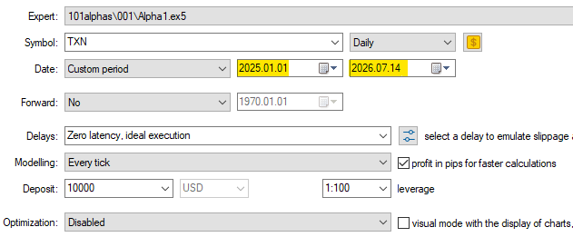
Fig. 10 - Backtest settings for TXN, from January 1, 2025, through the current day on the daily timeframe.

These are the backtest statistics for TXN.

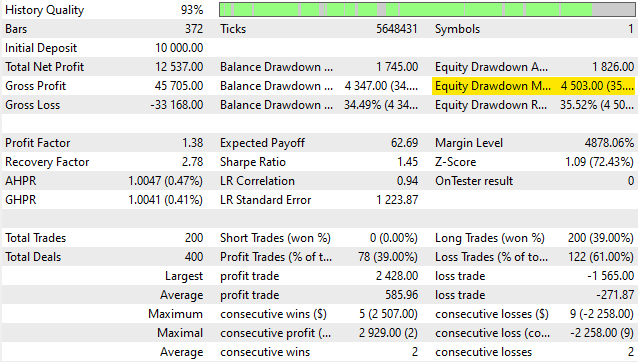
Fig. 11 - Backtest statistics for TXN

This is the balance/equity graph. Note the dangerously high relative drawdown.

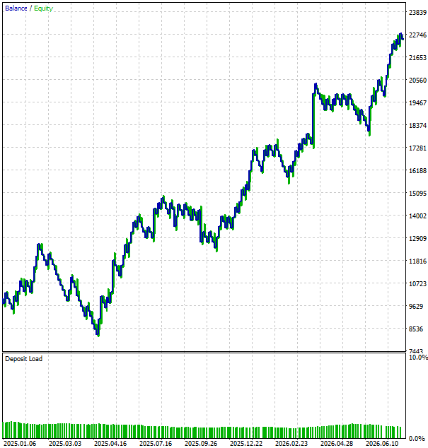
Fig. 12 - Balance/equity graph showing high drawdowns for TXN

These persistent drawdowns suggest that the risk management configuration may deserve some attention before advancing with this alpha. As noted, the stop-loss/take-profit were set to a conventional 1:2 ratio (25/50).

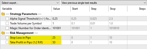
Fig. 13 - Screenshot showing the stop-loss and take-profit input values for TXN

A backtest like the above is what we usually do to evaluate a strategy or trading signal. To evaluate Alpha #1, we had to define the parameters of the strategy execution that are not part of the alpha. We defined the risk/return ratio with fixed stop-loss and take-profit distance in pips. If we change parameters, we modify the backtest results. So, we are not strictly evaluating the alpha. We are evaluating the alpha and its execution. 

Evaluation metrics

Before training models to generate new formulaic alphas, it is useful to review metrics that evaluate alphas without wrapping them in an arbitrary backtest strategy. If all that we want is to evaluate one, two, or ten alphas, it is fine to wrap them in an execution and run the traditional backtest as above. But what if we want to evaluate one hundred different alphas? 

Formulaic alphas were developed for this scenario: hundreds evaluating or thousands of alphas and eventually merging them into a single mega-alpha. This is our goal, and for this scenario, a backtest may not be the most practical evaluation method. Although the backtest will still be present near the end of the alpha qualification pipeline, there are more appropriate metrics for assessing an alpha’s predictive power without embedding it in a fully developed trading strategy.

The most fundamental of these metrics is the Information Coefficient (IC).

Information Coefficient (IC)

Information Coefficient (IC) is a simple and intuitive metric, defined as the Pearson correlation coefficient between the alpha values and the asset returns for a given period. It measures how close the alpha’s prediction value is to the asset returns, indicating the alpha’s forecasting ability and predictive power. The IC calculation is computationally cheap, fast, and reliable.

metrics.py

   @staticmethod
    def compute_daily_ic(df: pd.DataFrame, alpha_col: str = "alpha", target_col: str = "forward_returns") -> pd.Series:
        """
        Computes the daily Information Coefficient (IC).
        
        Definition: The Pearson correlation coefficient between the alpha values
        and the subsequent stock returns for each trading day across all assets.
        
        Intuition: Answers 'Does a higher alpha value linearly correspond to a higher return tomorrow?'
        """
        clean = df[[alpha_col, target_col]].dropna()
        
        def calc_pearson(group):
            if len(group) < 3 or group[alpha_col].std() == 0 or group[target_col].std() == 0:
                return np.nan
            return stats.pearsonr(group[alpha_col], group[target_col])[0]

        daily_ic = clean.groupby(level="time").apply(calc_pearson)
        daily_ic.name = "IC"
        return daily_ic.dropna()

This is the Alpha #1 Information Coefficient calculated for the same portfolio/universe of the backtest above. Since we are evaluating the daily timeframe, we extended the period to two years to have a more reliable sample of at least 500 days.

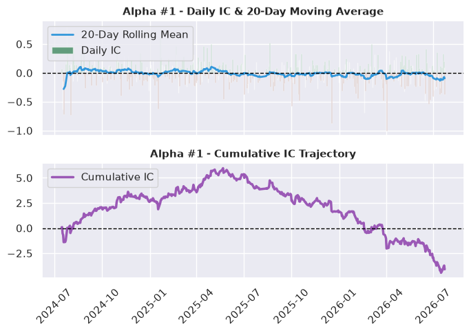
Fig. 14 - Plot of Alpha #1 Daily IC and cumulative IC

The IC trajectory in the second plot is the simple cumulative sum of daily ICs.

visualizer.py

cum_ic = daily_ic.cumsum()

The 20-day MA plot shows only a small shift in average IC around June 2025 (from slightly positive to slightly negative). The cumulative IC in the second plot makes the subsequent alpha decay clear. In hindsight, we see that it was a structural decay. The 20-day MA can only capture short-term variations around zero. It doesn’t track structural breaks. Because it continuously resets to its local baseline, it cannot capture the gradual change of predictive power over months. So, the analysis of this cumulative IC is paramount here.

Because the cumulative IC has a steady upward cumsum slope, we can say that, albeit weak, Alpha #1 showed real predictive power until around June 2025. After this period, the regime changed, and its decay began. We could use statistical methods for structural break detection to monitor this kind of alpha decay.

As noted, the IC is a fundamental metric. It is the basis for other metrics, including the Information Ratio (IR), and rank-based metrics that apply the Spearman correlation.

This is the terminal output of our basic alpha evaluation pipeline with metrics based on the Pearson correlation and rank-based ones based on the Spearman correlation.

--------------------------------------------------
  QUANTITATIVE EVALUATION SUMMARY: Alpha #1
--------------------------------------------------
  • Total Evaluation Days   : 498
  • IC Mean (Pearson)       : -0.0082
  • IC Standard Deviation   : 0.2055
  • ICIR (Pearson IR)       : -0.0400
  • Annualized ICIR         : -0.6350
  • t-statistic (IC)        : -0.8926
--------------------------------------------------
  • Rank IC Mean (Spearman) : +0.0219
  • Rank IC Std             : 0.2621
  • Rank ICIR               : +0.0835
  • Annualized Rank ICIR    : +1.3255
  • t-statistic (Rank IC)   : +1.8634
  • Hit Rate (RankIC > 0)   : 53.41%
--------------------------------------------------

We will be using some of these values in the brief analysis that follows.

Rank Information Coefficient (RankIC)

In the calculation of IC above, the SciPy stats.pearsonr function used the alpha signal values and the stocks' return percentages in the correlation formula. The calculation of the Rank IC using the SciPy stats.spearmanr function doesn’t use these values and percentages directly. Instead, it starts by sorting the stocks by their alpha score. Then, it assigns an integer to each element of this ordered set. The stock with the lowest alpha signal is assigned Rank 1; the second lowest alpha signal is assigned Rank 2; and so on, until all stocks are ranked by their respective alpha score. Another similar sorting is made, ranking the stocks by their returns, resulting in two ordered sets and two ranks. The Pearson correlation is then evaluated on these two ranks.

The result is that, while the IC measures the linear relationship between raw alpha values and stock returns, the Rank IC measures what the mathematicians call a monotonic relationship between their ranks. The Rank IC is about the order, not the exact price distance. It evaluates the sorting power of our signals, which is crucial for defining long/short positions for the highest/lowest ranks, respectively.

In the Rank IC, the impact of any single stock is minimized, but a single stock that, for any reason, experienced a peak may severely distort the IC evaluation. We can see the impact of these outliers in the evaluation summary. The IC mean is negative (-0.0082), while the Rank IC mean is positive (+0.0219). The alpha is ordering the stocks with relative success, but the low-alpha stocks (the outliers) diminished the Pearson correlation.

It is worth noting that both IC and Rank IC are useful, because the IC gives us the magnitude of the prediction, which reflects in the useful cumulative IC plot we saw above.

metrics.py

   @staticmethod
    def compute_daily_rank_ic(df: pd.DataFrame, alpha_col: str = "alpha", target_col: str = "forward_returns") -> pd.Series:
        """
        Computes the daily Rank Information Coefficient (Rank IC).
        
        Definition: The Spearman rank correlation (Pearson correlation applied to ranks)
        between alpha values and subsequent returns for each trading day across all assets.
        
        Intuition: Answers 'Does the alpha correctly rank assets from worst to best return,
        even if the relationship is non-linear or contains extreme outliers?'
        """
        clean = df[[alpha_col, target_col]].dropna()

        def calc_spearman(group):
            if len(group) < 3 or group[alpha_col].std() == 0 or group[target_col].std() == 0:
                return np.nan
            return stats.spearmanr(group[alpha_col], group[target_col])[0]

        daily_rank_ic = clean.groupby(level="time").apply(calc_spearman)
        daily_rank_ic.name = "RankIC"
        return daily_rank_ic.dropna()

Similar with the IC, the cumulative Rank IC in the second plot below is the simple cumulative sum of daily rank ICs.

visualizer.py

cum_rank_ic = daily_rank_ic.cumsum()

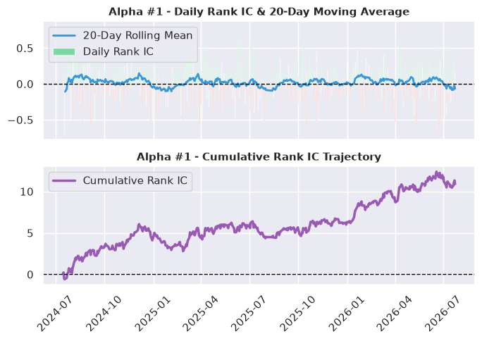
Fig. 15 - Plot of Alpha #1 Rank IC and cumulative Rank IC

The difference between IC and Rank IC stands out in the cumulative Rank IC plot. We lost the structural break information, but we can see that, except for periods with plateaus and drawdowns, the alpha has preserved its sorting capability in the last two years. That is, even when the signal direction began to decay in mid-2025, an increase/decrease in the alpha signal was followed by an increase/decrease in stock returns.

The forward return by quantile can help to understand what the cumulative Rank IC alone cannot make explicit.

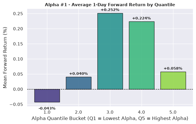
Fig. 16 - Plot of Alpha #1 average 1-day forward return by quantile

To a higher alpha signal, we expect a corresponding higher return. So, an ideal alpha would always plot growing steps from the lowest alpha quantile (Q1) through the highest alpha quantile (Q5). That is, it would show a strictly monotonic scale. But the plot shows that the stocks in Q3 and Q4 performed better than those in Q5.

Q1 (-0.043%)  <  Q2 (+0.040%)  <  Q3 (+0.252%)  >  Q4 (+0.224%)  >  Q5 (+0.058%)

The alpha correctly identifies the stocks to be avoided, those with negative returns (Q1), but fails to separate the most promising stocks from the average ones. This is why we cannot say that the alpha has preserved its ranking power all the time, but only for periods without plateaus and drawdowns in the cumulative Rank IC plot above.

In practical trading terms, if we were to use these alpha ranks to buy the 20% top-performing stocks, and sell the 20% bottom-performing ones, which is a common application for these ranks, we would be misguided on the long leg.

The limitations of the Alpha #1 are visually condensed in the Rank IC distribution plot below.

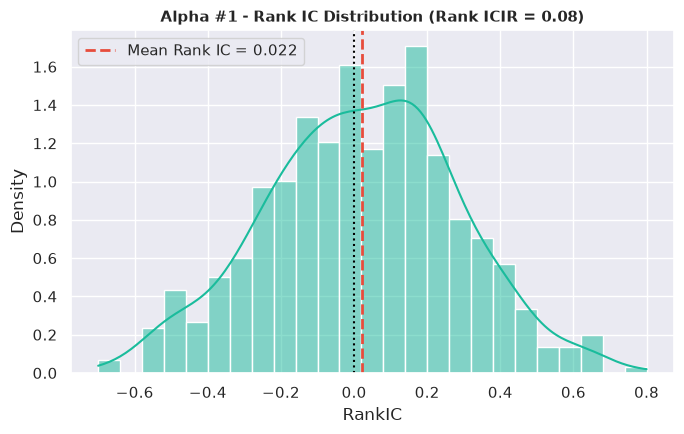
Fig. 17 - Plot of Alpha #1 Rank IC distribution

Note the wide bell shape. It indicates a wide standard deviation from the mean. Here, the mean is our signal, while the standard deviation is our noise. The Mean Rank IC is relatively small (+0.0219), and the Rank IC standard deviation is relatively large (0.2621). This results in a low ICIR (-0.04), as we saw in the summary above.  

The ICIR is the Information Ratio. 

Information Ratio (ICIR)

The Information Ratio (ICIR) is the core metric for a high-quality, stable alpha. It is a measure of the signal-to-noise ratio, defined as the IC’s mean divided by the IC’s standard deviation.

metrics.py 

   @staticmethod
    def compute_icir(daily_ic: pd.Series) -> float:
        """
        Computes the Information Ratio (ICIR).   
        Definition: mean(IC) / std(IC) over time.
        Intuition: Assesses the consistency and stability of predictive power. 
        A high mean IC with low volatility yields a high ICIR (good stability).
        """
        if len(daily_ic) < 2 or daily_ic.std() == 0:
            return 0.0
        return float(daily_ic.mean() / daily_ic.std())

To obtain a better signal-to-noise ratio, we would want the standard deviation to be smaller (which would result in a narrower distribution) and the Mean Rank IC to be greater. This would give us a higher Information Ratio. Our low signal-to-noise ratio is evident in the Information Ratio over a 60-day rolling window.

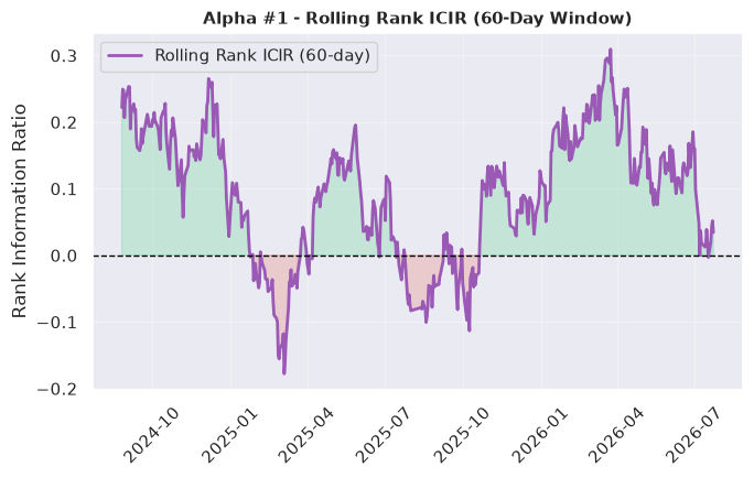
Fig. 18 - Plot of Alpha #1 rolling ICIR for a 60-day window

We can also see in this plot the structural break we have detected in the cumulative IC analysis, the alpha decay that started around June 2025. The rolling ICIR degradation started in the same period.

Since the rolling ICIR is based on the Pearson correlation (over raw alpha values and stock returns), it is sensitive to outliers, as we saw above in the IC and cumulative IC calculations. Imagine a stock with a very low alpha score for a given day. If, for any reason (a very positive unexpected earnings announcement, for example), this stock shows a price spike, the event would have a relatively high impact on the Pearson correlation between alpha scores and stock returns for that day. One popular technique for minimizing this relatively high impact of extreme values (outliers) is what statisticians call winsorization. For our purposes here, it is better to keep this distortion explicit, at least for now.

Rank Information Ratio (Rank ICIR)

Similar with IC Rank, the ICIR Rank is based on the alpha values and stock returns ranks, not on the raw values.

metrics.py 

   @staticmethod
    def compute_rank_icir(daily_rank_ic: pd.Series) -> float:
        """
        Computes the Rank Information Ratio (Rank ICIR).
        
        Definition: mean(RankIC) / std(RankIC) over time.
        
        Intuition: Measures the stability of rank prediction consistency across time.
        """
        if len(daily_rank_ic) < 2 or daily_rank_ic.std() == 0:
            return 0.0
        return float(daily_rank_ic.mean() / daily_rank_ic.std())

We see that the ranking power oscillates but remains valid most of the time.

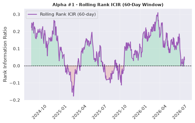
Fig. 19 - Plot of Alpha #1 rolling Rank ICIR for a 60-day window

While the Rolling ICIR above shows the structural break that caused the alpha decay around June 2025, the Rank ICIR shows that the Alpha #1 ranking power oscillates, is noisy, and prone to severe drawdowns, but it remains valid most of the time.

The annualization magnifies the difference between ICIR (-0.6350) and Rank ICIR (+1.3255) because it scales the daily results by the square root of the number of trading days.

metrics.py

   @staticmethod
    def compute_annualized_icir(daily_ic: pd.Series, annual_trading_days: int = 252) -> float:
        """
        Computes the Annualized Information Ratio (ICIR).        
        Definition: ICIR_daily × √252
        
        Intuition: Scales daily ICIR to an annualized expectation, enabling comparison
        with industry benchmarks. A rule of thumb: annualized ICIR > 1.0 is commercially viable.
        """
        icir = AlphaMetrics.compute_icir(daily_ic)
        return float(icir * np.sqrt(annual_trading_days))


   @staticmethod
    def compute_annualized_rank_icir(daily_rank_ic: pd.Series, annual_trading_days: int = 252) -> float:
        """
        Computes the Annualized Rank Information Ratio.
        Definition: Rank ICIR_daily × √252
        """
        rank_icir = AlphaMetrics.compute_rank_icir(daily_rank_ic)
        return float(rank_icir * np.sqrt(annual_trading_days))

The t-stat

The t-stat indicates how confident we can be that the Rank IC of 1.86 we obtained for Alpha #1 was not obtained by chance. That is, how much of its predictive power is statistically real, not just an occasional sequence of luck. According to statisticians, if we calculate the Rank IC for 1000 alphas, nearly 50 of them will have a t-stat above 1.96 purely by chance. 

Because machine-learning signals are typically discovered in batches of hundreds or thousands, evaluation should target large alpha sets rather than a single alpha such as Alpha #1. In a 2015 paper[5], quantitative researchers suggest that, for a large number of alphas evaluated simultaneously and a 95% confidence level, the t-stat critical threshold should be a Rank IC of at least 2.5.

Almost two decades earlier, when most analyses were centered around manually discovered alphas, a t-stat above 1.96 was considered acceptable for the same confidence level.[6]

The expression parser

Attached to this article, you will find an expression parser that implements the two formulaic alphas used as examples here, Alpha #1 and Alpha #101. To experiment with other formulas, you must update this file.

expression_parser_lark.py 

"""
Expression Parser Module using Lark for an alternate parser implementation.

This module provides a parser that can parse and evaluate formula strings like:
"(rank(Ts_ArgMax(SignedPower(((returns < 0) ? stddev(returns, 20) : close), 2.), 5)) - 0.5)"
"""

from lark import Lark, Transformer
import pandas as pd
import numpy as np

Conclusion

We used algebraic expressions known as formulaic alphas to show how we can use the Information Coefficient (IC) and the Information Ratio (ICIR) to evaluate machine-learning-generated trading signals (alphas) before the regular backtest. The same formula was evaluated in a MetaTrader 5 regular backtest for comparison.

We also provided a sample expression parser implemented in Python for the two formulaic alphas discussed in the article, making it easy to expand the library for further developments.

The evaluation of machine-learning-generated signals (alphas) in a systematic and automated way is a pre-requisite for filtering and merging a large number of potentially weak signals in a single tradable portfolio.

References

[1] Zuckerman, Gregory. “The Man Who Solved the Market: How Jim Simons Launched the Quant Revolution”. Portfolio/Penguin, 2019.

[2] Tulchinsky, Igor, et al., editors. “Finding Alphas: A Quantitative Approach to Building Trading Strategies”. 2nd ed., Wiley, 2020.

[3] Kakushadze, Zura, and Willie Yu. “How to Combine a Billion Alphas”. SSRN Scholarly Paper No. 2739219. Social Science Research Network, February 27, 2016.

[4] Kakushadze, Z. “101 Formulaic Alphas.” arXiv:1601.00991, arXiv, 18 Mar. 2016. arXiv.org.

[5] Zhu, Caroline and Harvey, Campbell R. and Liu, Yan, …and the Cross-Section of Expected Returns (February 3, 2015)

[6] Grinold, Richard C., and Ronald N. Kahn. Active Portfolio Management: A Quantitative Approach for Producing Superior Returns and Controlling Risk. 2nd ed., McGraw-Hill, 1999

Keywords: quantitative trading; machine learning; formulaic alphas; MQL5; MetaTrader 5; backtest

Filename	Description
MQL5\Experts\FormulaicAlphas\Alpha1.mq5	Alpha #1 Expert Advisor
MQL5\Include\FormulaicAlphas\Alpha1.mqh	Alpha #1 header
MQL5\Include\FormulaicAlphas\AlphaOperators.mqh	Generic alpha operators header
MQL5\Include\FormulaicAlphas\BaseAlpha.mqh	Base alpha class header
MQL5\Include\FormulaicAlphas\CrossSectional.mqh	Generic cross-sectional header
MQL5\Include\FormulaicAlphas\UniverseManager.mqh	Generic universe manager header
MQL5\Files\FormulaicAlphas\settings\alpha1-backtest.ini	Backtest settings
MQL5\Files\FormulaicAlphas\settings\alpha1-optimization.ini	Optimizations settings
MQL5\Files\FormulaicAlphas\python\data_loader.py	Python script to load OHLC data from MetaTrader 5 terminal
MQL5\Files\FormulaicAlphas\python\evaluator.py	Python script to orchestrate data loader, parser, metrics computation, and plotting
MQL5\Files\FormulaicAlphas\python\expression_parser_lark.py	Python script for expression parsing using the lark parser toolkit
MQL5\Files\FormulaicAlphas\python\main.py	Main entry point Python script
MQL5\Files\FormulaicAlphas\python\metrics.py	Python script for metrics computation
MQL5\Files\FormulaicAlphas\python\visualizer.py	Python script in charge of plotting